Enhancing Retail Transactions: A Data-Driven Recommendation Using Modified RFM Analysis and Association Rules Mining

Abstract

Retail transactions have become an integral part of the economic cycle of every country and even on a global scale. Retail transactions are a trade sector that has the potential to be developed continuously in the future. This research focused on building a specified and data-driven recommendation system based on customer-purchasing and product-selling behavior. Modified RFM analysis was used by adding two variables, namely periodicity and customer engagement index; clustering algorithm such as K-means clustering and Ward’s method; and association rules to determine the pattern of the cause–effect relationship on each transaction and four types of classifiers to apply and to validate the recommendation system. The results showed that based on customer behavior, it should be split into two groups: loyal and potential customers. In contrast, for product behavior, it also comprised three groups: bestseller, profitable, and VIP product groups. Based on the result, K-nearest neighbor is the most suitable classifier with a low chance of overfitting and a higher performance index.

1. Introduction

In today’s dynamic economic landscape, retail transactions have gained prominence, particularly in the burgeoning e-commerce sector. As global e-commerce sales surge from USD 1.3 trillion in 2014 to an estimated USD 4.9 trillion in 2021, as reported by Statista [1,2], the retail sector reveals remarkable potential for continuous growth. As a result of this evolution, businesses are being compelled to adapt to ever-evolving consumer needs and are now fiercely competing to enhance services, using data-driven insights. This necessitates the development of customized recommendation and promotion systems tailored to individual consumer behaviors. In addition, extensive data analysis has become a cornerstone of retail research, driving advancements aimed at boosting sales figures. With the urgency of remaining competitive, retailers across the globe upgrade digital advertisements, perfect personalization strategies, and boost loyalty programs.

Among the various methods employed to enhance retail transactions, the RFM-based and clustering approaches have shown great effectiveness. Alfian et al. [3] analyzed customer-purchasing patterns using the RFM model and K-means algorithm to investigate customer loyalty. Chen et al. [4,5,6] utilized the RFM model as a behavioral basis for their studies. Their research integrated techniques such as K-means clustering and decision trees to analyze customer purchasing behavior [4]. By identifying the most profitable customers and predicting potential profitability using linear regression, multi-layer perceptron, and naïve Bayesian [5], they provided valuable insights for strategic decision making. Additionally, they employed dynamic time-series models and neural networks for customer lifetime value prediction, further enhancing the understanding of customer behavior [6].

Association rule mining is widely used in product recommendation systems [7,8,9]. Studies by Lin et al. [7], Raorane et al. [8], and Liu et al. [9] utilized association rules to analyze consumer-purchasing behavior and develop recommendation systems. Lin et al. [7] segmented consumer-purchasing and product-selling behavior using quintiles differentiation in RFM value calculation and carried out association rules analysis as the extension of the recommendation model. According to Raorane et al. [8], the whole dataset was used as inputs on association rules mining to study consumer segmentation and transaction patterns. It generated a list of general product recommendations based on the transactions. Liu et al. [9] found that modifying support and confidence threshold values on association rules influenced the extent of product recommendation analysis. Nevertheless, these studies encountered limitations such as the lack of correlation between customer–product behavior and the recommendation system, generic recommendations, and applicability to specific customer segments only.

Our study refers to specific product recommendations for each customer group that are segmented based on the customer-purchasing behavior and also tries to recognize the pattern of product-selling behavior for each product group. As a result, this research aims to develop a specific recommendation model based on customer-buying and product-selling behavior, as existing models have yet to account for these two characteristics fully. The modified RFM analysis with additional variables, namely periodicity and customer engagement index, enhance the system’s accuracy and effectiveness in identifying patterns that support a deeper understanding of customer behavior. The developed model presents a new approach to product recommendation for each customer or company’s marketing strategy recommendation. It recognizes the pattern of customer-buying and product-selling behavior using the modified RFM model, customer engagement index, and clustering. The ranked customer–product category relationship shows if there is any connection between each customer-buying and product-selling behavior. In this paper, association rules mining is compared with the results of classification based on the customer and product, oriented to develop a novel recommendation system applicable to the retail market.

2. Theoretical Framework

2.1. Modified RFM Model and Customer Engagement Index (CEI)

Customer centricity is essential for success in the dynamic world of retail, where companies strive to provide customized experiences and maximize marketing initiatives. The RFM model, initially introduced by Hughes [10], is a framework for analyzing and predicting customer behavior based on recency, frequency, and monetary attributes. How recently a customer made a purchase is referred to as their recency. Customers who recently made purchases are frequently thought of as being more involved and possibly as being worth more to a company. The frequency of a customer’s purchases over a specific time period is represented by frequency. Customers that make repeated purchases may be more loyal and spend more money overall. Money spent by consumers on purchases is known as their monetary expenditure. Customers that spend more money are typically more important to a company’s income. The capacity of RFM analysis to identify discrete consumer categories based on their transactional behavior has attracted much interest. Over the past two decades, the RFM model has undergone evolution by incorporating additional variables such as customer relationship length [11,12,13,14,15,16], time since first purchase [11], churn probability [11], and product category group information [12]. RFM models are swift to implement and effectively capture customer characteristics, making them widely applicable in customer analysis and segmentation in various industries. Customers can be evaluated using actual values or the customer quintile differentiation method [7,13], which sorts customers into five equal quintiles based on RFM variables. The weighting of model variables can be equal or different based on industry characteristics [14].

However, in this research, we did not use all of the variables that were mentioned above since not all of them are related to retail terminologies. Rather, we used the term “modified RFM” to explain any modification we proposed for the basic RFM model to have a clearer and deeper analysis, specifically from the retail perspective. Peter and Kocyigit [14] proposed incorporating a periodicity variable into the RFM model, which indicates the regularity of a customer’s visits or purchases at fixed intervals. Nevertheless, in this study, we also focused on measuring the engagement level for each customer since, regarding retail, the engagement of customers who come and purchase at retail stores also determines the level of sales and company profits.

Herein, we introduce a customer engagement index (CEI) as another metric to assess customer engagement. Customer engagement, referring to the ongoing interactions and participations between a business and its customers, focuses on understanding individual purchasing behavior across different touchpoints and channels. Jen et al. [15] emphasized that expected frenquency of customer interaction significantly contribute to a company’s revenue. However, the customer engagement index specifically relates to customer-purchase behaviour. This model utilizes the time intervals between purchases in a customer’s historical consumption data as a variable. The formula proposed by Su et al. [16] is calculated using maximum likelihood estimation (MLE) and weighted maximum likelihood estimation (WMLE) as follows:

$$CEI=\frac{ MLE-WMLE}{MLE}$$

(1)

$$MLE={\sum }_{i=0}^{n-1}{\sum }_{j=i+1}^n\mathsf{\Delta }{t}_{ij }$$

(2)

$$\mathsf{\Delta }{t}_{ij }=X_{j }-X_{i }+1$$

(3)

$$WMLE={\sum }_{i=0}^{n-1}{\sum }_{j=i+1}^n\mathsf{\Delta }{t}_{ij }\times W_{i }$$

(4)

In this method, the total average of intervals between each purchase period for each customer is calculated. Transaction weights ($W_i$) are based on their order, with closer transactions having a higher weight. The timing of each customer’s purchases is taken into account. Here, i represents a transaction, j represents a subsequent transaction, and n reflects the total number of transactions for each customer or the frequency of purchases during a specific period. X_j and X_i denote the transaction dates. Note that $\mathsf{\Delta }{t}_{ij}$ is incremented by 1 to include the current transaction date.

To calculate the sum of MLE, $\mathsf{\Delta }{t}_{ij}$ is the duration between two transactions or between the last transaction and a dummy research date. WMLE is the weighted approximation obtained by summing the product of $\mathsf{\Delta }{t}_{ij}\mathrm{a}\mathrm{n}\mathrm{d}{W}_i.$ A CEI value greater than 0 (CEI > 0) indicates high customer engagement or an active customer, while a CEI value less than 0 (CEI < 0) signifies low customer engagement or an inactive customer. However, for this research, we assume that the highest CEI value is normalized to 1, and the lowest value is normalized to 0. Figure 1 mentions the schematic diagram for calculating customer engagement activity, meaning that the more transactions completed by the customer, the higher the CEI. This also happens if the duration between pair of transactions is small enough. This denotes a frequent customer.

2.2. Unsupervised Machine Learning: Clustering and Association Rule Mining

This section focuses on two types of unsupervised machine learning: clustering and association rule mining. Clustering is a data science technique that identifies patterns within a dataset based on similarities and dissimilarities between different clusters. There are two broad categories of clustering methods: probability-model-based approaches and nonparametric approaches [17]. The K-means clustering algorithm, a classic and efficient method, randomly selects k sample points as initial cluster centers, calculates the distance between the remaining sample points and the initial centers, assigns each point to the nearest cluster, and iteratively updates the cluster centers until convergence [18].

The elbow method (EM) and silhouette validation index are commonly used to determine the optimal number of clusters and evaluate the quality of clustering. The EM formula calculates the sum of distances within each cluster and considers the number of points in each cluster [19]. On the other hand, the silhouette validation index, introduced by Rousseeuw [20], measures the proximity of each data point to others within the same cluster and evaluates how well clusters are separated. It is based on the distances between points within and between clusters. The optimal value of k corresponds to the maximum silhouette value, indicating a better partition of the data points [21].

The market basket analysis carried out in the 1970s and 1980s is the origination of association rules mining. To find patterns of frequently purchased commodities, researchers first looked at how shoppers behaved in supermarkets. Optimizing product positioning and advertising was intended to increase sales. In 1994, Agrawal and Srikant invented the apriori algorithm, regarded as one of the most important contributions to association rules mining. Using the “apriori property”, which stipulates that any non-empty subset of a frequent itemset must likewise be frequent, this approach finds frequent itemsets. The apriori technique significantly decreases the computational difficulty of locating frequent itemsets [22].

Association rule mining (ARM) is widely utilized in a multitude of industries, such as market basket research [8,23], stock market analysis [24], recommendation systems [7,19,22,25,26,27], healthcare [28,29], and more [30]. This powerful technique plays a pivotal role in aiding organizations in making informed decisions [8,22,25,26], improving customer experience [7,19], and implementing preventive strategies [28,29]. Data mining identifies frequent itemsets (groups of items that frequently appear together) and generates explanations for them. The rules are expressed as “if-then” statements, where the antecedent is the presence of the items, and the consequent is the element likely to occur with the antecedent. The itemset support refers to the frequency of occurrence of an itemset in a dataset. The itemset percentage represents the percentage of itemsets in a transaction compared to all transactions. The confidence level, indicating the rule’s reliability, is determined by the ratio of transactions containing both the antecedent and consequent items to transactions containing only the antecedent [22,23].

2.3. Supervised Machine Learning: Classification

This section discusses the practical application of supervised machine learning algorithms, specifically focusing on classification techniques such as decision trees, bagging, AdaBoost, and K-nearest neighbors (KNN). Classification algorithms play a crucial role in predicting outcomes on new data by analyzing labeled training data, providing valuable insights, and supporting decision making across various disciplines. Each classification method offers unique working principles and benefits that we will explore further [18].

Decision trees, versatile machine learning models for classification and regression tasks, employ a hierarchical tree-like structure. Each internal node represents a feature and threshold, while leaf nodes represent classes or predicted values. This simple yet powerful structure facilitates the identification of key variables influencing customer segmentation. Decision trees create homogeneous subsets by recursively partitioning data based on feature thresholds, making them easy to comprehend and visualize [23]. Additionally, their transparency helps uncover patterns and customer groups more likely to be classified as “high-value”.

In cases where improved classification accuracy is required, ensemble methods like AdaBoost and bagging come into play. Both methods aim to enhance predictive accuracy and robustness by combining the predictions of multiple base models [18]. Bagging trains multiple instances of the same base model on different subsets of the training data [24,25], while AdaBoost focuses on misclassified samples and assigns higher weights to them during training [24,26]. Doing so allows weaker models to adapt and improve over time. Bagging reduces model variance while maintaining or improving bias, making it effective for small datasets or models prone to overfitting [25]. On the other hand, AdaBoost reduces model bias while maintaining or improving variance, making it suitable for more complex models [24].

The idea behind AdaBoost lies in iteratively assigning higher weights to misclassified instances, making them more influential in subsequent training rounds. Initially, all data points in the training dataset are given equal weights. The first weak learner is trained using the initial sample weights and evaluated on the trained data. Misclassified samples are identified, and their weights are increased. These weights emphasize the importance of each instance during the training process. Since AdaBoost focuses on improving weak learners’ performance (such as shallow decision trees), the weights of misclassified samples are increased during each training cycle, making them more influential in the subsequent training rounds. Such a process is repeated for a predefined number of iterations or until the desired level of accuracy is achieved. The final prediction is obtained by averaging or voting on the predictions of each model, creating a weighted mixture of the weak learners’ forecasts [24,26].

Bagging, enhanced by random forests, significantly improves classification performance through ensemble methods. The process involves training multiple instances of the same base model on different subsets of the training data obtained through bootstrapping—a random sampling technique with replacement. The bagging algorithm randomly selects N instances with replacements from a training dataset with N instances. Each subset, called a “bootstrap sample”, is applied to train a separate base model. Since each base model is trained on a different bootstrap sample, they are relatively independent. In bagging, diversity is essential, as it reduces overfitting and increases robustness overall. A final prediction is calculated by averaging the predictions made by each tree. Random forest is particularly effective for handling high-dimensional data and complex issues, as it lowers overfitting risk, improves accuracy, and ranks the priority features. Due to its effectiveness and reliability, random forest has gained popularity in various classification problems [24,27,28].

Machine learning uses the classification and regression algorithm K-nearest neighbors (KNN). It operates under the tenet that related data points frequently have the same label or value. Based on a selected distance metric (such as Euclidean distance), KNN determines the “K” closest data points in the training set given a new data point. For classification tasks, the algorithm then selects the most prevalent class among these neighbors as the forecast; for regression tasks, it averages their values. KNN is straightforward, flexible in terms of data distributions, and useful for small- to medium-sized datasets [23].

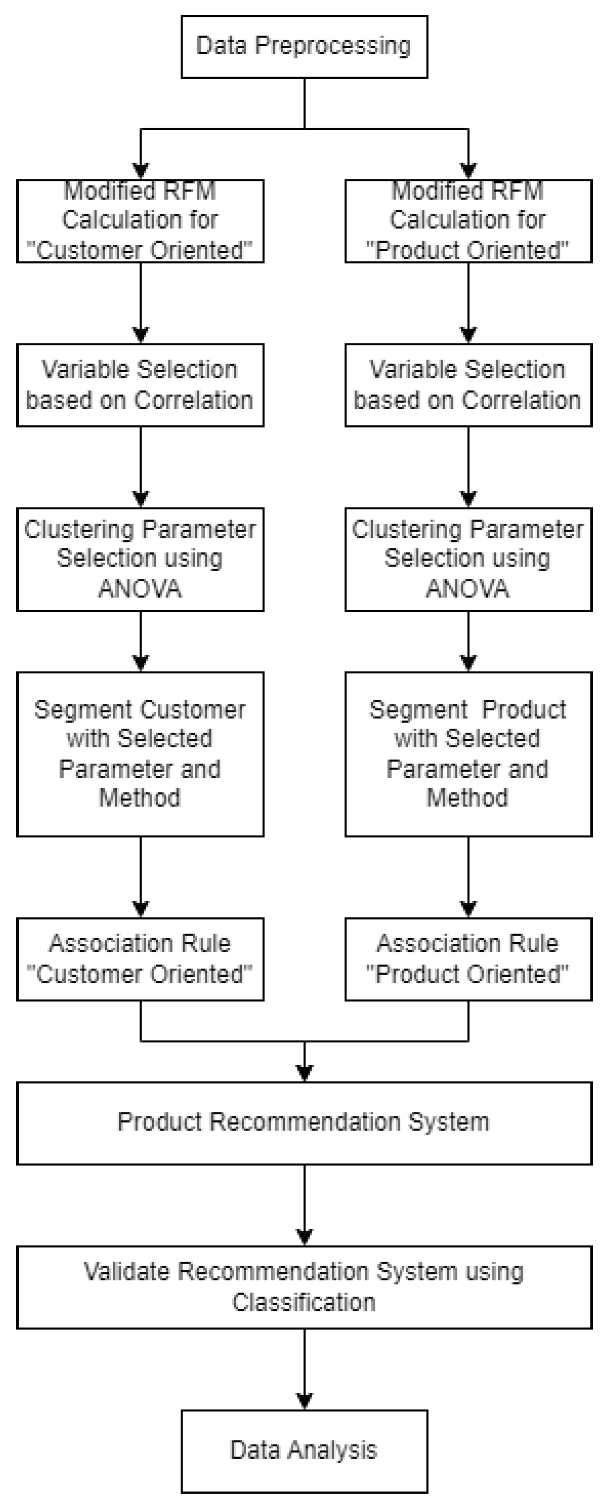
3. Research Methodology

This study aims to develop a product recommendation system that utilizes previous transaction data to suggest potential customer purchases. By employing clustering models, the study explores the correlations between customer groups and their purchases of various products to uncover meaningful customer characteristics.

In this study, we initially applied a modified RFM model with customer engagement index (CEI) to transform customer transaction data into R-values, F-values, M-values, p-values, and CEI values. These values were then categorized into two groups: customer-oriented and product-oriented. Correlation values were calculated for each group, and several models were selected for further analysis. The experimental design involves clustering based on four variables: models, clustering methods, clustering performance metrics, and the number of clusters. The output of the correlation calculation determined the combination variables. The clustering method variables employed Ward’s method and K-means clustering. Metrics such as the silhouette index (Sil), Calinski–Harabasz (CH) index, and Davies–Bouldin (DB) index were used to evaluate clustering performance.

Additionally, the number of clusters resulting from the clustering process was compared. Analysis of variance (ANOVA) and analysis of mean (ANOM) approaches identified variables significantly impacting the clustering step. These variables were then used to segment the customer-oriented and product-oriented groups. Association rules were utilized to identify correlations between customers’ purchases of different products, allowing for the grouping highly correlated products and increased profitability for the supermarket. This approach also provides insights into customer buying behavior within each product group. The antecedents and consequents of the association rules for customer buying behavior were employed to generate a product recommendation system using classification algorithms such as random forest classifier, a combination of AdaBoost algorithm or bagging algorithm with decision tree classifier, and K-nearest neighbor. The association rule mining (ARM) results were divided into training and testing groups to evaluate the performance of each classifier and validate the product recommendation system. The research framework is depicted in Figure 2 4.

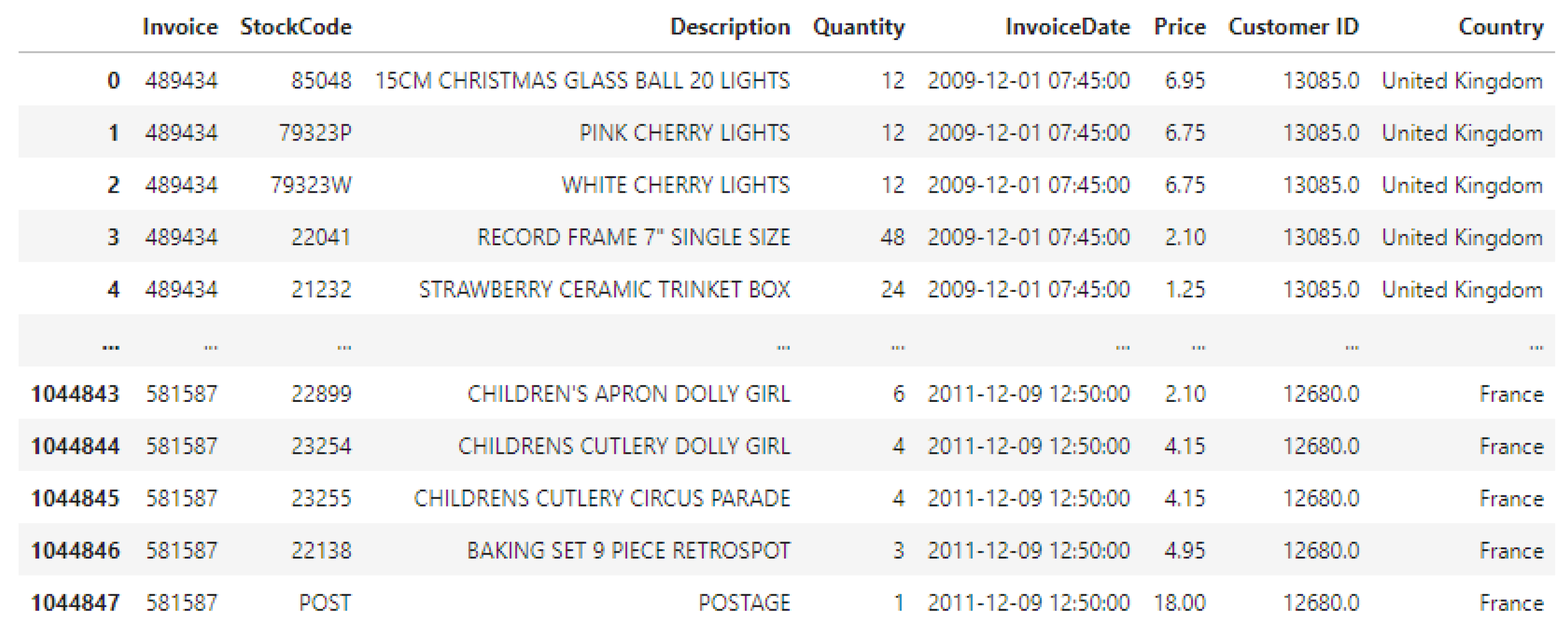
3.1. Data Description and Preprocessing

The present study analyzed a retailing mart database consisting of 5870 members. The dataset used for analysis was “online_retail_II.csv”, which contains 1,044,848 transactions spanning from December 2009 to December 2011. The dataset includes eight variables: invoice, stockcode, description, quantity, invoice date, price, customer ID, and country. Four variables were selected for this study, including customer ID, which represents the customer identity number associated with each transaction.

3.2. Modified RFM Value Calculation

The study focuses on calculating RFMCEIP (recency–frequency–monetary–customer engagement index–periodicity) variables. Firstly, the recency value was calculated as the number of days since each customer’s last purchase. Secondly, the frequency value was determined by counting the number of invoices for each customer, indicating the number of items purchased in each transaction. The monetary value was obtained by summing up the total spending of each customer. Periodicity is the average duration deviation between transaction times and was calculated using the formula (5).

$$Periodicity=stdev\left(\mathsf{\Delta }{t}_i, \mathsf{\Delta }{t}_{i+1}\dots ..\mathsf{\Delta }{t}_n\right)$$

(5)

where t_i denotes the date corresponding to the ith visit of the customer; last but not least, the CEI was calculated as Formulas (1)–(4) to show the activeness of each customer to visit the shop. We used the RFMCEIP calculation results to assess the correlation levels between customer- or product-oriented variables. The selection of variable combinations aimed to minimize the risk of collinearity, wherein variables with strong correlations (above 0.8) may have similar patterns, and one variable can represent the others.

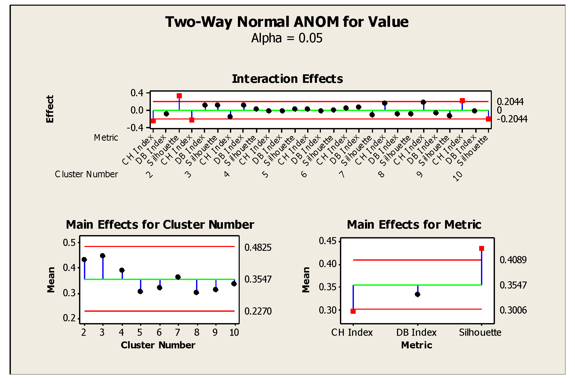
3.3. Clustering Parameter Selection and Clustering

The selection process involved using the ANOVA approach with four factors: combination variables (referred to as models), clustering methods (K-means clustering and Ward’s method), clustering performance metrics (Sil, CH, and DB), and the number of clusters ranging from 2 to 10. The ANOVA approach generated significant factors, and further analysis was conducted using the ANOM approach to determine the best approach for the clustering steps. Both ANOVA and ANOM approaches were performed for both groups. After obtaining the results, the clustering step was executed using the best approach determined from the previous analysis. The performance index of selected metrics was evaluated to determine the correct and optimal number of clusters. The segmentation results were then analyzed and labeled based on the characteristics of each group.

3.4. Association Rules Mining

The apriori algorithm, which identifies frequent itemsets and association rules in relational databases, was employed for customer and product behavior segmentation. It begins by identifying frequent individual items and extends to larger itemsets based on their frequency in the database. The resulting frequent itemsets determine association rules that highlight general trends. The output includes antecedents and consequents, indicating the cause–effect relationship between combinations related to products or customer behavior. This causal effect served as input for the next step.

3.5. Validation for Product Recommendation System

Classification-based algorithms such as random forest classifier, a combination of bagging or Adaboost algorithm with decision tree classifier, and K-nearest neighbor were employed. The causality results obtained from the ARM analysis for each behavior segmentation were divided into antecedents (X) and consequents (Y). The data were split into 80% training and 20% testing data [29]. The performance index, including precision, recall, and f1-score, was used to evaluate the accuracy of each classifier and validate the recommendation system based on customer transactions and purchased products.

4. Results

This section may be divided into subheadings. It should provide a concise and precise description of the experimental results, their interpretation, as well as the experimental conclusions that can be drawn.

4.1. Data Description and Preprocessing

A dataset called “online_retail_II.csv” was used in this study. The dataset contains 1,044,848 transactions from December 2009 to December 2011 and eight variables, including invoice, stockcode, description, quantity, invoice date, price, customer ID, and country. Among those eight variables, four were retained.

Table 1. Basic Information for Dataset.

Items	Notes
Invoice	Bill ID for each of the customer’s transaction
StockCode	Product ID number
Description	Product name
Quantity	Number of products being purchased by the customer
InvoiceDate	Customer purchasing time
Price	The amount of money spent by consumers for each product
Customer ID	Customer membership ID number
Country	Location of delivery

shows the basic information of the dataset.

The dataset has a variable called description, which is mentioned in Table 1 as the name of the product. In this study, each product was labeled as a group of product categories so that further analysis of product category behavior could be applied, especially to bring an effective recommendation system. The product categories were divided into 18 groups, including as lights, decoration, storage, kitchen utensils, accessories, clothes, candles and incense, stationary, toys, bags, gifts, utensils, bank, bedroom utensils, living room utensils, and discount. There is a “discount” category since the discount transactions are noted in the dataset with a minus value on the “price” column. Figure 3 showed the sample of dataset that been utilized in this research.

4.2. Modified RFM Value Calculation

Researchers commonly utilize the RFM model to analyze customer behavior. As part of this study, we introduced two additional variables, customer engagement index (CEI) and periodicity, to enhance the analysis. The RFMCEIP was calculated from two distinct groups: one that focused on customers and one that focused on products. Customer-oriented groups allowed us to understand customer behavior based on their transactions. On the other hand, the product-oriented group concerned how products perform in sales and transactions. We used 1 January 2012 as a dummy research date to facilitate analysis. This approach enabled us to gather meaningful data and draw valuable conclusions from our study.

Table 2. RFMCEIP Customer-Oriented Value Result.

Customer ID	Recency (Days)	Frequency (Times)	Monetary (USD)	CEI	Periodicity (Days)
12346.0	348	25	170.40	0.997	60.68
12347.0	25	222	554.57	0.980	19.06
12348.0	98	51	193.10	0.994	57.55
12349.0	41	175	1480.44	0.986	18.66
12350.0	333	17	65.30	0.997	0.00
...	...	...	...	...	...
18283.0	26	938	1651.60	0.932	34.97
18284.0	454	28	91.09	0.996	0.00
18285.0	683	12	100.20	0.998	0.00
18286.0	499	67	286.30	0.992	0.00
18287.0	65	155	346.34	0.985	73.21

shows the result of the RFMCEIP calculation for the customer-oriented group. This table also shows the CEI value normalized with uniform distribution from 0 until 1, meaning 0 is the least-buying customer, and 1 is the most-buying customer. For example, for customer 12346.0, the result showed that the recency equaled 348 days, frequency equaled 25 times, monetary equaled USD 170.40, CEI equaled 0.997, and periodicity equaled 60.68 days. According to the results, it had been 348 days since customer 12346.0’s last purchase in the store. In the past two years, the customer completed transactions 25 times, with spending equal to USD 170.40. The customer was included in the group of customers who are quite active in transactions, while the average duration between each purchase was 60.68 days.

Table 3. RFMCEIP Product-Oriented Value Result.

Description	Recency (Days)	Frequency (Times)	Monetary (USD)	CEI	Periodicity (Days)
15 cm Christmas Glass Ball 20 Lights	76	437	3387.15	0.926	8.36
Pink Cherry Lights	76	230	1478.00	0.926	12.53
White Cherry Lights	76	216	1378.70	0.928	1.62
Record Frame 7” Single Size	76	323	792.95	0.942	3.02
Strawberry Ceramic Trinket Box	76	1859	2297.12	0.608	0.92
...	...	...	...	...	...
Gin and Tonic Diet Metal Sign	76	37	92.94	0.991	0.45
Set of 6 Ribbons Party	76	13	37.17	0.997	0.96
Silver and Black Orbit Necklace	76	1	2.95	1.000	0.00
Cream Hanging Heart T-light Holder	76	7	20.25	0.998	0.32
Paper Craft, Little Birdie	76	1	2.08	1.000	0.00

shows the result of the RFMCEIP calculation for the product-oriented group. This table also shows the CEI value normalized with uniform distribution from 0 until 1, meaning 0 is the least-sold product, and 1 is the most-sold product. For example, for the product 15 cm Christmas Glass Ball 20 Lights, the result showed that recency equaled 76 days, frequency equaled 437 times, monetary equaled USD 3387.15, CEI equaled 0.926, and periodicity equaled 8.36 days. According to the results, it had been 76 days since the Product 15 cm Christmas Glass Ball 20 Lights was last purchased. The product was sold 437 times in the past two years, generating a total income of USD 3387.15. The product was included in the most-sold products in transactions, while the average duration between each purchase was 8.36 days.

4.3. Clustering Parameter Selection and Result of Cluster

Subsequently, selection of parameters for the clustering process was necessary. Using customer- and product-oriented RFMCEIP results, correlation analysis was conducted to determine the appropriate model. The objective was to identify variable relationships within the range of 0.2 to 0.8 and eliminate variables that exhibit the highest and lowest correlations to minimize the risk of multicollinearity.

Table 4. Correlation Matrix for RFMCEIP Customer-Oriented Group.

Customer	Recency	Frequency	Monetary	CEI	Periodicity
Recency	1.00	−0.22	−0.17	0.20	−0.30
Frequency	−0.22	1.00	0.89	−1.00	0.01
Monetary	−0.17	0.89	1.00	−0.88	0.01
CEI	0.20	−1.00	−0.88	1.00	−0.01
Periodicity	−0.30	0.01	0.01	−0.01	1.00

presents the correlation matrix for the RFMCEIP customer-oriented group. It reveals strong positive correlations between “frequency” and “monetary” variables (0.89), indicating that customers who make more frequent purchases tend to spend higher amounts.

The customer engagement index (CEI) refers to customer participation and interactions with the business. It consists of two main aspects: the time between one purchase and the next and the frequency of purchases. The correlation test results showed that the CEI index exhibits strong negative correlations with the frequency (−1.00) and monetary (−0.88) variables. Such can be observed in cases where a customer was more active in the past than they are currently and has made almost no repurchases recently. Such purchasing behavior could be an indication that the customer needs to be more fully engaged and consistently active with the business. Conversely, a CEI index greater than 0 indicates that this customer has been quite active recently and shows more proactive repurchasing behavior compared to the past.

The analysis also shows several weak correlations. The “recency” variable has a weak positive correlation with the CEI index (0.20), indicating a slight connection between recent interactions and higher customer involvement. Conversely, the correlation between recency and monetary is weaker (<0.2), suggesting a less robust relationship, while the periodicity also shows weak correlations with other variables, suggesting limited relationships with recency, frequency, and monetary variables and CEI index. Thus, at least one variable from each combination was selected for the model, including the RFM, MCEIP, and FMP models.

Table 5. Correlation Matrix for RFMCEIP Product-Oriented Group.

Product	Frequency	Monetary	CEI	Periodicity
Frequency	1.00	0.02	−0.99	−0.23
Monetary	0.02	1.00	−0.35	−0.08
CEI	−0.99	−0.35	1.00	0.24
Periodicity	−0.23	−0.08	0.24	1.00

presents the correlation matrix for the RFMCEIP (RFM with customer engagement index and periodicity) in a product-oriented context. Notably, recency variables were not included due to constant recency values for all products. Several interesting correlations were found. First, frequency and CEI index have a significant negative correlation (−0.99). Products that were once more popular now sell less frequently. Also, the correlation between product frequency and periodicity is moderately low (−0.23). Products with a higher purchase frequency have longer sales intervals. Despite being sold frequently, some products do not maintain regular sales intervals.

Furthermore, the correlation between monetary and CEI is negative but relatively weak (−0.35). In other words, higher-value products may have a lower customer engagement index. In other words, high profits sometimes indicate better customer engagement with the business. The relationship between monetary and periodicity is minimal. However, the relationship between CEI and periodicity is positive, with a 0.24 value. Accordingly, products with higher customer engagement index values have more regular purchase intervals. A popular product is more likely to generate sales consistently. As a result, at least one variable from each combination, including the RFM model, MCEIP model, and FMP model, was selected for the model. These correlations provide valuable insights into product-oriented customer behavior, aiding in the development of effective marketing strategies and decision-making processes.

This study investigated the significance of each factor’s impact on the selected models. To achieve this,

Table 6. Experiment Factors for ANOVA.

Model	Metrics	Methods	Cluster Number
RFM	Silhouette Index Calinski–Harabasz Index Davies–Bouldin Index	K-Means Clustering Ward’s Method	2	3	4
			5	6	7
			8	9	10
MPCEI	Silhouette Index Calinski–Harabasz Index Davies–Bouldin Index	K-Means Clustering Ward’s Method	2	3	4
			5	6	7
			8	9	10
FMP	Silhouette Index Calinski–Harabasz Index Davies–Bouldin Index	K-Means Clustering Ward’s Method	2	3	4
			5	6	7
			8	9	10

presents the experiment factors utilized in the analysis of variance (ANOVA). Careful consideration was given to the chosen metrics, clustering methods, and cluster numbers to evaluate the models’ performances comprehensively. The study involved three distinct models: RFM (recency, frequency, and monetary), MPCEI (monetary, periodicity, and CEI index), and FMP (frequency, monetary, and periodicity). Every model was assessed using several metrics, such as Sil, CH, and DB. By conducting the ANOVA analysis, the researchers aimed to identify any significant differences or correlations between these factors and the model’s performance. The ANOVA results provided valuable insights into the relative importance of each factor in the clustering process, enabling a better understanding of the strengths and weaknesses of each model under various conditions and configurations.

Furthermore,

Table 7. ANOVA Result for Customer-Oriented Group.

Source	DF	F	p-Value
Model	2	149.74	0.000
Method	1	6.88	0.011
Cluster Number	8	4.7	0.000
Metrics	2	423.32	0.000
Model and Method	2	0.53	0.592
Model and Cluster Number	16	0.8	0.680
Model and Metric	4	260.08	0.000
Method and Cluster Number	8	0.4	0.914
Method and Metric	2	6	0.004
Cluster Number and Metric	16	6.57	0.000
Model and Method and Cluster Number	16	0.11	1.000
Model and Method and Metric	4	0.47	0.761
Model and Cluster Number and Metric	16	0.21	0.999

presents the ANOVA results for the customer-oriented group. The analysis indicates that all four variables significantly affected the clustering process. Several factors show statistically significant effects on the clustering process. For example, the “model” factor exhibits a highly significant effect on customer-oriented clustering (F = 149.74, p < 0.001). This result suggests that the choice of clustering models, such as RFM, MPCEI, or FMP, significantly influences the overall performance of the clustering process.

Similarly, the “method” and “cluster number” factors show a significant impact. The result for the “method” factor (F = 6.88, p = 0.011) indicates that the specific clustering method employed, such as K-means clustering or Ward’s method, plays a crucial role in determining the quality and accuracy of the resulting clusters. The result for the “cluster number” factor (F = 4.7, p < 0.001) indicates that the number of clusters chosen for the analysis has a substantial effect on the clustering outcomes and the ability to group customers based on their characteristics effectively. Additionally, the “metrics” factor significantly influences customer-oriented clustering (F = 423.32, p < 0.001). The choice of evaluation metrics, such as Sil, CH, or DB, greatly affected the assessment and comparison of different clustering models’ performance.

In addition, there are significant effects generated based on the interaction of the factors. For example, the combination of “model” and “metrics” showed a significant result (F = 260.08; p = 0.000), meaning that the selection of both factor combinations also gives a significant effect. This result suggests selecting both combinations, such as RFM, MPCEI, or FMP, with CH, DB, or Sil simultaneously. Another example is the “method” and “metrics” combination, which also showed significant results (F = 6.000, p = 0.004), meaning that the combination of both factors gives a significant additional interaction effect to the clustering quality. The result implies selecting both simultaneously, such as K-means clustering or Ward method, with CH, DB, or Sil. Finally, the “cluster number” and “metrics” combination caused a significant effect on clustering quality (F = 6.57, p = 0.000). This result shows that if the combination of both factors is chosen, a better clustering result will be obtained, for example, CH, DB, or Sil combined with the number of clusters from 2 to 10.

Moreover, the combinations of model and metrics, method and metric, and cluster number and metric exhibit significant interaction effects on the clustering process. Based on these results, further analysis using the analysis of mean approach was conducted to determine the optimal parameters for the clustering process.

Figure 4 presents the analysis of the mean for the model and metric in the customer-oriented group. Based on the literature review, the Davies–Bouldin index (DB) and silhouette index (Sil) are considered better when following the “bigger is better” rule. Conversely, the Calinski–Harabasz index (CH) is better when following the “less is better” rule. Applying these rules, the MCEIP model demonstrates the best result, exhibiting the highest Sil and the lowest CH. Both models yielded similar results for the DB. The RFM model is thus rejected due to its poorer performance with a high CH value and a low DB value. Furthermore, the choice of metric significantly impacted the evaluation of clustering results. In this study, SI was chosen instead of CH for its simplicity and compatibility with the “bigger is better” rule, which provides a clearer representation of clustering performance.

Figure 5 illustrates the results of the analysis of mean for method and metric in the customer-oriented group. The findings indicate no significant difference between K-means clustering and Ward’s method in terms of the clustering method. However, K-means clustering was selected for its flexibility and ease of use.

Figure 6 displays the results of the analysis of mean for cluster number and metric in the customer-oriented group. The analysis shows no significant effect of the “cluster number” factor, necessitating further analysis using the Sil metric to determine the optimal number of clusters for customer segmentation.

Table 8. ANOVA Result for Product-Oriented Group.

Source	DF	F	p
Model	2	136.82	0.000
Method	1	4.4	0.040
Cluster Number	8	2.01	0.059
Metrics	2	357.58	0.000
Model and Method	2	0.04	0.959
Model and Cluster Number	16	1.48	0.135
Model and Metric	4	82.2	0.000
Method and Cluster Number	8	0.13	0.997
Method and Metric	2	4.55	0.014
Cluster Number and Metric	16	19.39	0.000
Model and Method and Cluster Number	16	0.07	1.000
Model and Method and Metric	4	1.06	0.384
Model and Cluster Number and Metric	16	0.59	0.881

presents the results of ANOVA for the product-oriented group. It reveals that three variables, except for the cluster number, significantly affected the clustering process. Additionally, the combinations of model and metrics, method and metric, and cluster number and metric exhibit significant interaction effects. As a result, an extended analysis using the mean approach was conducted to determine the best parameters for the clustering process.

Figure 7 demonstrates the results of the analysis of the mean for the model and metric in the product-oriented group. Similar to the previous analysis, the DB and Sil are considered better when following the “bigger is better” rule, while the CH is better when following the “less is better” rule. Based on these rules, the FMP model demonstrates a good result, displaying a high DB and a low CH, with a slightly higher Sil value than the MCEIP model. The RFM model is thus rejected due to its inferior performance, characterized by a high CH and a low DB. It is also evident that the choice of metric significantly affected the evaluation of clustering results. Sil was chosen over CH to simplify the research process, particularly for determining the number of clusters and evaluating clustering performance in the subsequent steps.

Figure 8 shows the results of the analysis of mean for method and metric in the product-oriented group. The analysis revealed no significant difference between K-means clustering and Ward’s method in terms of the clustering method. Therefore, K-means clustering was chosen based on its flexibility and ease of use.

Figure 9 displays the results of the analysis of mean for cluster number and metric in the product-oriented group. The analysis indicates no significant effect of the “cluster number” factor, requiring further analysis using the Sil metric to determine the optimal number of clusters for product segmentation.

Figure 10 illustrates the results of the Sil analysis for the customer-oriented and product-oriented groups. As mentioned, Sil follows the “higher is better” rule, implying that a higher value signifies better clustering performance. Better performance in the clustering process indicates the ability of clusters to effectively group data based on their characteristics. Figure 10a demonstrates that the highest Sil value is obtained with two clusters, indicating that it is preferable.

Figure 11 presents the results of the elbow method using the sum of squared error with Euclidean distance for the product-oriented group. The figure shows a significant drop from one cluster to three clusters, and from three clusters onwards, the decrease becomes more stable. The finding indicates that the optimal number of clusters representing the data characteristics in the product-oriented group is three. Figure 12 depicts the clustering results for both the customer-oriented and product-oriented groups using K-means clustering.

Table 9. Customer Segmentation Interpretation.

	Cluster 1 (Potential Customer—1160 Cust)			Cluster 2 (Loyal Customer—4710 Cust)
	Monetary	CEI Index	Periodicity	Monetary	CEI Index	Periodicity
Min	3.450	0.000	2.110	0.000	0.691	0.000
Mean	538.380	0.986	132.770	399.096	0.988	16.022
Max	56,337.290	0.999	495.750	13,916.340	1.000	72.610

illustrates the results of clustering segmentation, which categorizes customer behavior into two groups: potential customers and loyal customers. Cluster 1, referred to as potential customers, exhibited a lower customer engagement index (CEI) mean value (0.986) compared to cluster 2 (0.988), indicating less activity. Additionally, the average duration between transactions (periodicity) for cluster 1 (132.77 days) was longer than that of cluster 2 (16.022 days). These results validate the CEI calculation, as cluster 2 tended to make repeat transactions every 16–17 days, while cluster 1 made repeat purchases after 132 days. In terms of monetary value, cluster 1 (USD 538.38) had a higher mean value than cluster 2 (USD 399.096), suggesting that customers in cluster 1 are more profitable for the company, whereas cluster 2 is more profitable in terms of transaction frequency. In the actual world, potential customers spend less, are less active, and wait longer between purchases than loyal customers. However, with the correct marketing plan, potential customers can turn into devoted patrons. A loyal customer is usually found as a frequent customer, while a potential customer will appear if there is any additional motivation, for example, if there is any promotion or needs at any certain time.

Table 10. Product Segmentation Interpretation.

	Cluster 1 (Best Seller—4870 Products)			Cluster 2 (Profitable—391 Products)			Cluster 3 (VIP—18 Products)
	Frequency	Monetary	Periodicity	Frequency	Monetary	Periodicity	Frequency	Monetary	Periodicity
Min	1.000	0.017	0.000	3.000	0.480	1.239	3.000	0.570	0.425
Mean	155.932	454.953	10.050	15.163	58.806	91.096	900.722	14,780.086	249.059
Max	2045.000	12,528.000	51.309	2099.00	10,013.57	231.316	5016.000	146,269.190	498.507

presents the results of clustering segmentation for product behavior, categorizing products into three groups: best-selling, profitable, and VIP. Cluster 1 represents the best-selling products, with a higher transaction frequency mean (155.932 times) than cluster 2 (15.163 times). Additionally, cluster 1 showed a shorter average duration (10.050 days) than cluster 2 (91.096 days). Regarding monetary value, cluster 2 (USD 58.806) was more profitable than cluster 1 (USD 454.953), considering the respective transaction frequencies. Cluster 3 is an outlier in the data, displaying extremely high values compared to the other clusters. Cluster 3 exhibited an average transaction frequency of 900.722 times and an average duration of 249.059 days. The monetary value for cluster 3 was significantly higher, reaching USD 14,780.086. Comparing the frequency and monetary values, Cluster 3 generated substantially greater income than the other two groups. Best-selling items are typically inexpensive and sold in great quantities in the real world. Office supplies are one of the best-selling items since they are frequently purchased. Products with a high selling value but a low sales volume are known as VIP products. This category includes household furniture and appliances in general. Among them are profitable products with a medium frequency of sales and a reasonably medium monetary value. This category of merchandise includes apparel, accessories, and kitchenware.

4.4. Association Rules Mining

The results in

Table 11. Top Ten Association Rule for Customer-Oriented Group (each cluster).

Cluster	Antecedents	Consequents	Support	Confidence	Lift
Potential	Toys	Stationery, Storage	20.047%	65.421%	1.672
Potential	Stationery, Storage	Toys	20.047%	51.228%	1.672
Potential	Bag, Gift	Stationery, Decoration, Kitchen Utensils	21.443%	78.506%	1.630
Potential	Stationery, Decoration, Kitchen Utensils	Bag, Gift	21.443%	44.520%	1.630
Potential	Bag, Decoration, Gift	Stationery, Kitchen Utensils	21.443%	81.409%	1.626
Potential	Stationery, Kitchen Utensils	Bag, Decoration, Gift	21.443%	42.835%	1.626
Potential	Decoration, Kitchen Utensils, Gift	Stationery, Bag	21.443%	55.465%	1.619
Potential	Stationery, Bag	Decoration, Kitchen Utensils, Gift	21.443%	62.606%	1.619
Potential	Decoration, Bag, Kitchen Utensils	Stationery, Gift	21.443%	51.945%	1.614
Potential	Stationery, Gift	Decoration, Bag, Kitchen Utensils	21.443%	66.626%	1.614
Loyal	Stationery, Kitchen Utensils	Bag, Storage	20.43%	47.11%	1.599
Loyal	Bag, Storage	Stationery, Kitchen Utensils	20.43%	69.35%	1.599
Loyal	Bag, Kitchen Utensils	Stationery, Storage	20.43%	50.82%	1.593
Loyal	Stationery, Storage	Bag, Kitchen Utensils	20.43%	64.03%	1.593
Loyal	Stationery, Decoration	Bag, Storage	20.41%	46.38%	1.575
Loyal	Bag, Storage	Stationery, Decoration	20.41%	69.30%	1.575
Loyal	Stationery, Storage	Bag, Decoration	20.41%	63.98%	1.562
Loyal	Bag, Decoration	Stationery, Storage	20.41%	49.83%	1.562
Loyal	Stationery, Bag	Kitchen Utensils, Storage	20.43%	71.24%	1.550
Loyal	Kitchen Utensils, Storage	Stationery, Bag	20.43%	44.44%	1.550

show the ten best association rules for the customer-oriented dataset. Each rule corresponds to a specific cluster. Several patterns of co-occurring items appear in customers’ transactions, indicating possible relationships between products frequently purchased together. The “potential” cluster shows the strongest associations between “toys”, “stationery”, “storage”, “bag”, “gift”, “decoration”, and “kitchen utensils”. Customers in this cluster are 65.421% confident they will buy “toys” when they also purchase “stationery” and “storage.” Similarly, they express 78.506% confidence in buying a combination of “bag”, “gift”, “stationery”, “decoration”, and “kitchen utensils”. These strong association rules suggest that offering or promoting these product combinations as bundles or in proximity may encourage more sales and enhance customer satisfaction. However, the “loyal” cluster contains association rules involving “stationery”, “kitchen utensils”, “storage”, “bag”, and “decoration”. Customers in this cluster are 69.35% confident in purchasing “stationery” and “kitchen utensils” when they also purchase “bags” and “storage”. Their confidence in buying a combination of “stationery”, “bags”, “kitchen utensils”, and “storage” is also 70.24 percent. Based on these findings, it is likely that customers in this cluster prefer specific combinations of products. Offering these combinations as tailored packages or promotions may increase brand loyalty and repeat purchases.

Table 12. Association Rule for Product-Oriented Group (each cluster).

Cluster	Antecedents	Consequents	Support	Confidence
Best-Seller	Loyal	Potential	91.62%	93.22%
Best-Seller	Potential	Loyal	91.62%	98.88%
Profitable	Potential	Loyal	88.52%	100%
Profitable	Loyal	Potential	88.52%	88.52%
VIP	Potential	Loyal	88.52%	100%
VIP	Loyal	Potential	88.52%	88.52%

displays the association rules for the product-oriented group, describing the likelihood of each customer group purchasing the same product category due to the influence of another customer group. For instance, in the best-seller product category, the potential–loyal relationship has a confidence level of 98.88%, higher than the loyal–potential relationship (93.22%). This finding indicates that potential customers have a higher chance of influencing loyal customers to purchase the same product category. Otherwise, in another two clusters, both agree that potential–loyal associations are more confident (100%) than the association of loyal–potential (88.52%). These results can be used as a strategy to generate additional income and increase customer engagement caused by the association effect of each customer in terms of purchasing and promoting any product. For example, the company could offer coupons or additional discounts to potential customers to purchase best-seller products, thereby increasing the likelihood of loyal customers also purchasing in the same category. Additionally, in this situation, the effects of word-of-mouth marketing carried out by each antecedent to the consequents may play a crucial role. For instance, in the case of profitable and VIP products, it is more effective if the company prioritizes marketing the product to potential customers first so that they can automatically suggest the same product to loyal customers.

4.5. Validation for Product Recommendation System

The recommendation system based on association rules was validated and applied using a classifier algorithm. Four different algorithms, including a random forest classifier, a combination of decision tree with bagging algorithm, a combination of decision tree with AdaBoost algorithm, and a K-nearest neighbor, were trained and evaluated in an experiment.

Table 13. Product Recommendation Implementation and Validation with Classifier.

Classifier	Model	Accuracy	Precision	Recall	F1-Score
Random Forest Classifier	Training	0.094	0.44	0.1	0.12
	Testing	0.042	0.1	0.06	0.07
Decision Tree + Bagging Algorithm	Training	0.088	0.4	0.1	0.12
	Testing	0.051	0.1	0.07	0.07
Decision Tree + AdaBoost Algorithm	Training	0.096	0.43	0.13	0.12
	Testing	0.051	0.11	0.09	0.09
K-Nearest Neighbor	Training	0.06	0.25	0.1	0.13
	Testing	0.025	0.24	0.08	0.11

presents the performance of these algorithms. The combination of the decision tree with the AdaBoost algorithm generated the most accurate result based on the training model, with results on accuracy (0.096), precision (0.43), recall (0.13), and F1-scores (0.12). On the other hand, there were also good results for the testing model (accuracy = 0.051, precision = 0.11, recall = 0.09, F1-score = 0.09). By comparing to the other, both models shoed a big deviation, meaning that while the training model can predict accurately, the algorithm cannot classify correctly on the testing model, which symbolizes an overfitting problem. This also occurred with the random forest classifier, which on the training model had similar results as the decision tree and AdaBoost algorithm (accuracy = 0.094, precision = 0.44, recall = 0.1, F1-score = 0.12). Meanwhile, the testing model proved to be an overfit model (accuracy = 0.042, precision = 0.1, recall = 0.06, F1-score = 0.07). The decision tree and bagging algorithm combination gave slightly worse results regarding the training model compared to the previous models (accuracy = 0.088, precision = 0.4, recall = 0.1, F1-score = 0.12).

On the other hand, this combination showed a lower deviation of each metric than the two previous models (accuracy = 0.051, precision = 0.1, recall = 0.07, F1-score = 0.07), meaning that in this process, a combination of the decision tree and bagging algorithm showed a better result in overcoming the overfitting problem. Although all of them exhibited overfitting, with higher results in the training model compared to the testing model in terms of accuracy, the K-nearest neighbor algorithm demonstrated a good-enough result regarding the metrics both in the training set (accuracy = 0.06, precision = 0.25, recall = 0.1, F1-score = 0.13) and the testing set (accuracy = 0.025, precision = 0.24, recall = 0.08, F1-score = 0.11). The K-nearest neighbor performed better on the testing model, which delivered a non-overfitting classifier, so K-nearest neighbor is the most suitable classifier for implementing this recommendation system. While K-nearest neighbor was not the best-performing classifier in this study, the deviation of the training and testing result is the least when compared with another classifiers. In the real-world situation, by using K-nearest neighbor, the prediction will be more precise, stable, and reliable based on the training set. By predicting the recommendation as precisely as the purchasing behavior, the rate of transaction might be increased.

5. Discussion

This research aimed to develop a data-driven recommendation system based on customer-purchasing and product-selling behavior. We enhanced the commonly used RFM analysis by incorporating the periodicity and customer engagement index (CEI) variables to achieve this. The RFM, MCEIP, and FMP models were selected for clustering parameter selection, with RFM as the baseline model. The MCEIP model predicted the customer activity percentage based on the average transaction duration and spending. In contrast, the FMP model focused on profit estimation per transaction, frequency, and predicting the time of future transactions. The periodicity variable represents the average transaction duration and can be used to anticipate when customers will make their next purchase.

Table 14. Relationship Between Customer and Product.

Product	Customer	Amount of Transaction	Percentage
Best-Seller	Loyal	582,581	74.74
	Potential	176,809	22.68
VIP	Loyal	2674	0.34
	Potential	1171	0.15
Profitable	Loyal	13,194	1.69
	Potential	3019	0.39

presents the relationship between the customer-oriented and product-oriented groups. It shows that most transactions (74.74%) come from loyal customers purchasing best-selling products. Although these products have a high sales frequency, they generate relatively lower income, indicating that loyal customers prefer lower-priced items. The second largest percentage is the best-seller products purchased by the potential customers. Since the product has a lower income or, on the other hand, it is not quite expensive, it is suitable for potential customers to buy. Promotion for best-seller products to potential customers is recommended by giving a coupon or having a buy–get promotion. Since it is also associated with loyal customers, one suggestion might be to work with the larger effect by targeting the potential customers and indirectly targeting the loyal ones. Profitable products lead to many transactions (1.69 and 0.39) compared with VIP ones (0.34 and 0.15). Since the average periodicity for profitable products is approximately three months, we can consider it a quintile product that will be bought with a seasonal pattern every 3 months. Giving some promotion or discount in the non-peak season is a great way to increase the number of purchases, especially for potential customers.

On the other hand, while a profitable product has more transactions with a shorter periodicity, the VIP product is recognized as a special group of products that generates the highest monetary value but with less frequency and longer periodicity. Since then, loyal or potential customers might purchase the VIP item for occasional purposes or at any event. A promotion for the VIP product might work by giving a slight discount during the peak season. Also, giving a big discount or combining it with another product type as a complementary promotion in the non-peak season will create more transactions, especially for potential customers.

The recommendation list derived from Table 11 was generated based on product combinations within each invoice. The association rules determine the highest likelihood of recommended product combinations for future transactions. Implementing this recommendation system, which relies on customer-purchasing behavior, is critical and requires the latest database updates within a data-driven system. It accounts for potential shifts in customer-purchasing and product-selling behavior. By segmenting customers based on their tendencies and characteristics, specific products can be recommended due to transaction and customer similarity.

6. Conclusions

This research endeavored to construct a precise and targeted recommendation system rooted in an in-depth understanding of customer-purchasing and product-selling behaviors. Our approach hinges on the analysis of customer-purchasing patterns, enabling us to categorize customers based on their distinctive characteristics and tailor our promotional strategies accordingly. Simultaneously, we delve into product-selling behavior, shedding light on the characteristics that drive customer interest and profitability.

To achieve this, we augmented the RFM analysis with periodicity and CEI variables and use clustering algorithms to group customers and products based on their similarities. ANOVA and ANOM analyses were conducted to select the optimal clustering parameters, including models, metrics, methods, and cluster numbers. The MCEIP model, K-means clustering, and silhouette index were employed for the customer-oriented group. In contrast, the product-oriented group utilized the FMP model, K-means clustering, and silhouette index.

The results indicate that customer behavior can be divided into two groups, namely loyal and potential customers, while product behavior is categorized into three groups: best-seller, profitable, and VIP products. Association rules were analyzed to identify purchasing combinations within product categories, which were subsequently utilized in a classifier-based recommendation system. Among the classifiers tested, K-nearest neighbor demonstrated the most suitable performance, with low overfitting probability and high performance index. In the real-world situation, by using K-nearest neighbor, the prediction will be more precise, stable, and reliable based on the training set. By predicting the recommendation as precisely as the purchasing behavior, the rate of transaction might be increased. This study also shows the suggestions for a marketing strategy that can be applied for the specific segment, either from a customer or product perspective, while both can be applied and affect each other to improve customer loyalty and retail sales amount.

Although our data-driven approach enables us to offer tailored and specific recommendations, it also poses some limitations. The analysis is based on a secondary dataset, which raises the possibility of producing disparate results based on actual transaction data. As a result, we should continue to investigate our findings in practice to verify them. To increase the robustness of our recommendation system, we acknowledge the importance of expanding the horizons of our research by exploring alternative classifier options. Several strategic considerations drove our choice of data from 2009 to 2011 relative to our data selection. Firstly, the data were obtained from a company that analyzes long-term customer behavior. We gained valuable insights from this historical dataset about customer and product interactions. Our analysis, however, does not solely depend on historical data from this period. Instead, we leveraged this historical dataset as a foundational platform to develop and validate models, frameworks, and methodologies designed for broad applicability. Regardless of the dataset’s vintage, it was designed for adaptability and application to current and future data. This older dataset was selected for empirical research and as a basis for establishing a suitable recommendation system model. Nevertheless, as stated in the conclusion, our findings should be applied to real-world datasets for thorough evaluation.

References

1. Chevalier, S. Retail E-Commerce Sales Worldwide from 2014 to 2026, Statista, Hamburg. 2022. Available online: https://www.statista.com/statistics/379046/worldwide-retail-e-commerce-sales/ (accessed on 29 August 2023).
2. Sabanoglu, T. Estimated Value of the In-Store and e-Commerce Retail Sales Worldwide from 2022 and 2026, Statista, Hamburg. 2022. Available online: https://www.statista.com/statistics/443522/global-retail-sales/ (accessed on 29 August 2023).
3. Alfian, T.; Sandi, A.; Raharjo, M.; Putra, J.L.; Ridwan, R. Clustering Kesetiaan Pelanggan E-Ritel Dengan Model Rfm (Recency, Frequency, Monetary) Dan K-Means. J. Pilar Nusa Mandiri 2018, 14, 239. [Google Scholar]
4. Chen, D.; Guo, K.; Ubakanma, G. Predicting Customer Profitability over Time Based on RFM Time Series. Int. J. Bus. Forecast. Mark. Intell. 2015, 2, 1. [Google Scholar] [CrossRef]
5. Chen, K.; Hu, Y.H.; Hsieh, Y.C. Predicting Customer Churn from Valuable B2B Customers in the Logistics Industry: A Case Study. Inf. Syst. E-Bus. Manag. 2015, 13, 475–494. [Google Scholar] [CrossRef]
6. Chen, D.; Guo, K.; Li, B. Predicting Customer Profitability Dynamically over Time: An Experimental Comparative Study. In Proceedings of the Pattern Recognition, Image Analysis, Computer Vision, and Applications: 24th Iberoamerican Congress, CIARP 2019, Havana, Cuba, 28–31 October 2019. [Google Scholar]
7. Lin, R.H.; Chuang, W.W.; Chuang, C.L.; Chang, W.S. Applied Big Data Analysis to Build Customer Product Recommendation Model. Sustainability 2021, 13, 4985. [Google Scholar] [CrossRef]
8. Raorane, A.A.; Kulkarni, R.V.; Jitkar, B.D. Association Rule-Extracting Knowledge Using Market Basket Analysis. Res. J. Recent Sci. 2012, 2277, 2502. [Google Scholar]
9. Liu, H.-W.; Wu, J.-Z.; Wu, F.-L. An App-Based Recommender System Based on Contrasting Automobiles. Processes 2023, 11, 881. [Google Scholar] [CrossRef]
10. Hughes, A.M. Boosting Response with RFM. Mark. Tools 1996, 5, 4–10. [Google Scholar]
11. Yeh, I.-C.; Yang, K.-J.; Ting, T.-M. Knowledge Discovery on RFM Model Using Bernoulli Sequence. Expert. Syst. Appl. 2009, 36, 5866–5871. [Google Scholar] [CrossRef]
12. Chang, H.-C.; Tsai, H.-P. Group RFM Analysis as a Novel Framework to Discover Better Customer Consumption Behavior. Expert. Syst. Appl. 2011, 38, 14499–14513. [Google Scholar] [CrossRef]
13. Miglautsch, J.R. Thoughts on RFM Scoring. J. Database Mark. Cust. Strategy Manag. 2000, 8, 67–72. [Google Scholar] [CrossRef]
14. Peker, S.; Kocyigit, A.; Eren, P.E. LRFMP Model for Customer Segmentation in the Grocery Retail Industry: A Case Study. Mark. Intell. Plan. 2017, 35, 544–559. [Google Scholar] [CrossRef]
15. Jen, L.; Chou, C.H.; Allenby, G.M. The importance of modeling temporal dependence of timing and quantity in direct marketing. J. Mark. Res. 2009, 46, 482–493. [Google Scholar]
16. Su, Z.X.; Liu, Y.Z.; Liu, H. A Customer Value-Based Framework for Database Marketing. J. Inf. Manag. 2013, 20, 341–366. [Google Scholar]
17. Nainggolan, R.; Perangin-angin, R.; Simarmata, E.; Tarigan, A.F. Improved the Performance of the K-Means Cluster Using the Sum of Squared Error (SSE) Optimized by Using the Elbow Method. J. Phys. Conf. Ser. 2019, 1361, 012015. [Google Scholar] [CrossRef]
18. Mahesh, B. Machine Learning Algorithms—A Review. Int. J. Sci. Res. 2019, 9, 381–386. [Google Scholar] [CrossRef]
19. Yıldız, E.; Güngör Şen, C.; Işık, E.E. A Hyper-Personalized Product Recommendation System Focused on Customer Segmentation: An Application in the Fashion Retail Industry. J. Theor. Appl. Electron. Commer. Res. 2023, 18, 571–596. [Google Scholar] [CrossRef]
20. Rousseeuw, P.J. Silhouettes: A Graphical Aid to the Interpretation and Validation of Cluster Analysis. J. Comput. Appl. Math. 1987, 20, 53–65. [Google Scholar] [CrossRef]
21. Liu, Y.; Li, Z.; Xiong, H.; Gao, X.; Wu, J. Understanding of Internal Clustering Validation Measures. In Proceedings of the 2010 IEEE International Conference on Data Mining, Sydney, NSW, Australia, 13–17 December 2010; pp. 911–916. [Google Scholar]
22. Agrawal, R.; Imieliński, T.; Swami, A. Mining Association Rules between Sets of Items in Large Databases. In Proceedings of the 1993 ACM SIGMOD International Conference on Management of Data—SIGMOD, New York, NY, USA, 1 June 1993; ACM Press: New York, NY, USA, 1993; pp. 207–216. [Google Scholar]
23. Ray, S. A Quick Review of Machine Learning Algorithms. In Proceedings of the 2019 International Conference on Machine Learning, Big Data, Cloud and Parallel Computing (COMITCon), Faridabad, India, 14–16 February 2019; pp. 35–39. [Google Scholar]
24. Awotunde, J.B.; Folorunso, S.O.; Imoize, A.L.; Odunuga, J.O.; Lee, C.-C.; Li, C.-T.; Do, D.-T. An Ensemble Tree-Based Model for Intrusion Detection in Industrial Internet of Things Networks. Appl. Sci. 2023, 13, 2479. [Google Scholar] [CrossRef]
25. Breiman, L. Bagging Predictors. Mach. Learn. 1996, 24, 123–140. [Google Scholar] [CrossRef]
26. Zhou, Y.; Qiu, G. Random Forest for Label Ranking. Expert. Syst. Appl. 2018, 112, 99–109. [Google Scholar] [CrossRef]
27. Breiman, L. Random Forest. Mach. Learn. 2001, 45, 5–32. [Google Scholar] [CrossRef]
28. Singh, N.; Bhatnagar, S. Machine Learning for Prediction of Drug Targets in Microbe Associated Cardiovascular Diseases by Incorporating Host-pathogen Interaction Network Parameters. Mol. Inform. 2022, 41, 2100115. [Google Scholar] [CrossRef] [PubMed]
29. Stojčić, M.; Banjanin, M.K.; Vasiljević, M.; Nedić, D.; Stjepanović, A.; Danilović, D.; Puzić, G. Predictive Modeling of Delay in an LTE Network by Optimizing the Number of Predictors Using Dimensionality Reduction Techniques. Appl. Sci. 2023, 13, 8511. [Google Scholar] [CrossRef]
30. Chen, D.; Sain, S.L.; Guo, K. Data Mining for the Online Retail Industry: A Case Study of RFM Model-Based Customer Segmentation Using Data Mining. J. Database Mark. Cust. Strategy Manag. 2012, 19, 197–208. [Google Scholar] [CrossRef]
Figure 1. Schematic Diagram of Customer Engagement Activity.
Applsci 13 10057 g001
Figure 2. Data Analysis Framework.
Applsci 13 10057 g002
Figure 3. The Sample of Dataset.
Applsci 13 10057 g003
Figure 4. ANOM Result for Model and Metric (Customer-Oriented Group).
Applsci 13 10057 g004
Figure 5. ANOM Result for Method and Metric (Customer-Oriented Group).
Applsci 13 10057 g005
Figure 6. ANOM Result for Cluster Number and Metric (Customer-Oriented Group).
Applsci 13 10057 g006
Figure 7. ANOM Result for Model and Metric (Product-Oriented Group).
Applsci 13 10057 g007
Figure 8. ANOM Result for Method and Metric (Product-Oriented Group).
Applsci 13 10057 g008
Figure 9. ANOM Result for Cluster Number and Metric (Product-Oriented Group).
Applsci 13 10057 g009
Figure 10. (a) Result of Silhouette Index for Customer-Oriented Group. (b) Result of Silhouette Index for Product-Oriented Group.
Applsci 13 10057 g010
Figure 11. Elbow Method Result for Product-Oriented Group.
Applsci 13 10057 g011
Figure 12. (a) Clustering Result for Customer-Oriented Group. (b) Clustering for Product-Oriented Group.
Applsci 13 10057 g012