Equilibrium Optimizer-Based Joint Time-Frequency Entropy Feature Selection Method for Electric Loads in Industrial Scenario

Abstract

A prerequisite for refined load management, crucial for intelligent energy management, is the precise classification of electric loads. However, the high dimensionality of electric load samples and poor identification accuracy of industrial scenarios make it difficult to be used in actual production. As such, this research presents a selection approach equilibrium optimizer-based joint time-frequency entropy feature selection method for electric loads in industrial scenarios to address these issues. The method first introduces entropy value features based on extracting time-frequency domain features and then uses an equilibrium optimizer (EO) to screen the joint feature set. A Chinese cement plant was chosen as the acquisition site for the experiments, and the low-frequency data from power equipment were gathered to form an original dataset for power analysis. The features screened by the EO were used as model inputs to verify the effectiveness of the EO on the joint feature set under K-nearest neighbor (KNN), support vector machine (SVM), decision tree (DT), random forest (RF), and discriminant analysis (DA) models. Experimental results show that introducing entropy value features for the joint feature set can significantly improve the classification performance. The average accuracy of the features screened by the EO was as high as 95.58% on SVM, while the computation time was 0.75 s. Therefore, for industrial electricity scenarios, the approach suggested in this research can enhance the identification accuracy of electric loads and significantly reduce the computation time of the model to a great extent. This has essential research significance for intelligent energy management in real industrial scenarios.

1. Introduction

Energy is an essential basis for the development of human society [1] and a key factor for economic expansion and the quality of life [2,3]. With the process of industrialization and population growth [4,5], energy demand is growing [6], and energy consumption has diversified and become complicated [7]. In energy consumption, electrical energy occupies a large proportion, reflecting a country or region’s industrialization level and technological innovation ability [8,9]. As a core component of electrical energy consumption, industrial electricity directly affects the efficiency and quality of industrial production and is more involved in environmental protection and energy conservation. Therefore, improving the efficiency of industrial power consumption [10] and optimizing the structure of industrial power consumption are important ways to promote sustainable economic and social development [11]. The study of electric load identification for industrial power consumption scenarios helps to optimize equipment configuration and scheduling strategies [12], reduce inefficient power and losses, improve energy utilization, and realize intelligent energy management [13].

At present, the application of electric load identification technology in energy management is receiving increasing attention [14]. Electricity load identification can provide necessary data support for application scenarios such as industrial power consumption [15], grid scheduling [16], virtual power plants [17], smart charging [18], and scenery collaboration [19]. In response to traditional algorithms’ low computational efficiency and identification accuracy, Wu et al. [20] proposed an event-based residential electric load identification algorithm. The combination of underdetermined decomposition and characteristic filtering methods is used to determine the specific harmonic retention of the filter output. This is used to achieve the purpose of load identification. The experiments use high-frequency current sampling data and monitor the occurrence of switching events based on intensity changes. The outcomes demonstrated that the algorithm has superior computational efficiency and identification precision compared to the conventional method. Rafiq et al. [21] introduced an extended short-term memory algorithm approach that employs a multi-feature subspace that has been demonstrated to be suitable for on-site measurement applications. In the presence of noise, the model was trained by multi-feature input space and mutual information and evaluated the performance in the ECO and UKDALE datasets. The evaluation results show that this method is better than the benchmark algorithm in terms of computational efficiency and scalability and can meet real-time requirements. Considering that introducing unknown electrical loads remains a challenge for accurate classification, Yin et al. [22] recommended a method for spatial convex packet overlap rate similarity calculation as a basis for identifying load types. A Siamese neural networks-based modeling approach was first applied to the low-dimensional feature space. Transfer learning was then introduced to learn and identify unknown electrical loads. The performance was experimentally verified with the residential dataset Plaid. The findings indicate that this approach has high precision in the recognition of unknown electric loads, which adds new power to the load monitoring technique. The industrial sampling frequency is much lower than that of the residential electricity scenario, resulting in fewer samples of electrical parameters collected within a fixed time duration and poorer sample quality, making studying industrial electric load identification more difficult. Luan et al. [23] validated the hidden Markov model (HMM) on the publicly available dataset HIPE and the Chinese brickyard dataset to address the research gap in load decomposition and classification in industrial scenarios. The results show that the variant algorithm improves over the benchmark. The identification of electric loads is widely studied but is currently focused on residential electricity scenarios. The industrial electricity scenario is more challenging to study due to the harsh sampling environment and diverse equipment types. Therefore, how to achieve accurate identification of electric loads in industrial electricity scenarios is an urgent problem.

The technical route of electric load identification usually includes feature extraction, feature selection, and equipment classification. For industrial power scenarios, extracting valuable features from low-frequency data and screening out the appropriate feature combinations from the joint feature set determine the effectiveness of equipment identification. YU et al. [24] used V-I trajectories and active power for feature extraction. To recognize power consumption categories, their algorithm employs Siamese neural networks to compute the V-I track similarities before comparing signatures in the feature library. The findings reveal that the suggested approach performs better than utilizing the raw power data alone. High-frequency data can be collected in residential electricity scenarios. Ghosh et al. [25] proposed an improved load identification method with the help of current harmonic characteristics of electrical loads. An intelligent identification method based on fuzzy rules detects and monitors a wide range of electrical loads. The proposed method enhances the accuracy of identifying several devices by considering the load characteristics on the power side. After determining the electrical parameters, feature types also need to be selected [26,27,28]. Yan et al. [29] suggested a recognition approach that combines time-frequency features. First, time and frequency domain features are extracted to construct fused features, then a random forest algorithm is employed to identify a significant subset of features, and finally, SVM is utilized as experiment classifier. To assess feasibility, a case study was performed using an authentic Irish dataset. The findings demonstrated that this method performs better with the introduction of frequency domain features. Tran et al. [30] put forward a feature selection approach founded on fuzzy entropy values and similar classifiers. The proposed method is effective in reducing noise. The results on the experimental dataset show that the classification accuracy is improved, and the computation time is reduced. Metaheuristic algorithms are a class of problem-independent optimization techniques that explore and develop the entire search space based on the principle of multiple iterations [31,32]. EO algorithms, as metaheuristics, are derived from the dynamic mass equilibrium model of the control container and have been used in several fields [33]. Faramarzi et al. [34] introduced the equilibrium optimizer algorithm in 2020. In order to demonstrate the superiority of the EO, metaheuristic algorithms of various types and periods of development were selected for comparison, and 58 mathematical benchmark functions and three engineering problems were experimentally examined. In terms of performance, the algorithm obtains optimal results and has the utmost efficacy across a wide range of problems, outperforming traditional and newly developed algorithms. Sayed et al. [35] combined EO and chaos theory and performed experiments in the UCI machine learning library. The findings indicate that the algorithm can identify the optimal subset of features and acquire the best classification outcomes while selecting the least number of features. Considering the dimensional disaster generated by many features, TOO et al. [36] proposed an EO-based variant of the algorithm, which is considered a wrapper-based approach for feature selection. There were sixteen datasets used to validate the effectiveness. The results show that the algorithm performs well regarding fitness value, accuracy, and feature size compared to other metaheuristics. Thus, extracting the joint time-frequency entropy features of power samples can balance both local and global features of the signal. EO has superior performance in terms of feature dimensionality and classification accuracy, and has also been confirmed to generalize well over different datasets and classifiers. Displaying feature distribution with box and whisker plots can effectively represent feature information [37,38].

Having taken these factors into account, this paper put forward a novel electric load feature selection method for the low-frequency data collected in industrial power consumption scenarios. This method introduces entropy value features based on extracted time-frequency domain features and then uses the EO to screen in the joint feature, which helps achieve accurate classification of industrial power loads. The structure of this paper is as follows. In Section 2, the flowchart for the procedure proposed in this paper is first described succinctly. Then, the data sources for this experiment, the time-frequency entropy features of various electrical loads, the principle of the algorithm of EO, and the application of the EO to the joint feature selection of electric loads are presented. Section 3 presents the specific experiments. First, the power curve and cleaning effect are shown, then the joint features are extracted according to the feature principle, and next, the joint feature set is screened using the EO. Based on this, the authors verify the validity of this study with five classifiers. Section 4 demonstrates the necessity and effectiveness of the experimental steps by comparison. The classification effects before and after feature extraction are first compared, and then the performance of different feature combinations is compared to demonstrate the superiority of the joint feature set. To assess the dependability of the EO, the authors select four metaheuristic algorithms for the comparison of feature selection effects. Finally, the authors conclude by summarizing their study and anticipating future research.

2. Proposed Methodology for Industrial Electric Load Identification

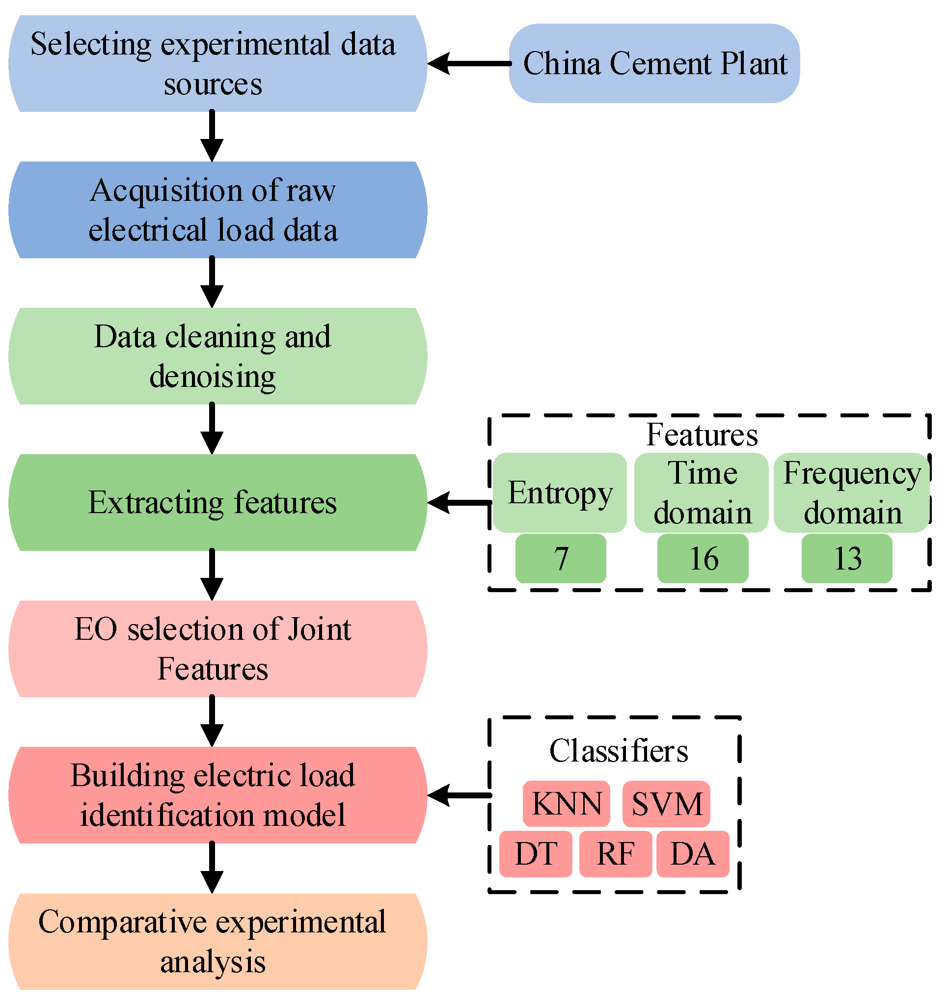
Figure 1 illustrates the exact experimental procedure of this paper. The experiment selects the load data of a Chinese cement plant, which includes the active and reactive power of nine pieces of equipment. First, the electric power data are cleaned according to the original power signal data sampling. Subsequently, entropy value features are introduced based on extracted time-frequency domain characteristics to enhance the quality of the joint feature set. Finally, the EO screens the feature categories of the electric loads and uses the selected feature subsets as model inputs for equipment classification. To verify the feasibility of introducing entropy value features and EO feature selection in industrial electric load identification, the authors also conduct comparative experiments to demonstrate the necessity and superiority of the experimental steps.

2.1. Data Introduction

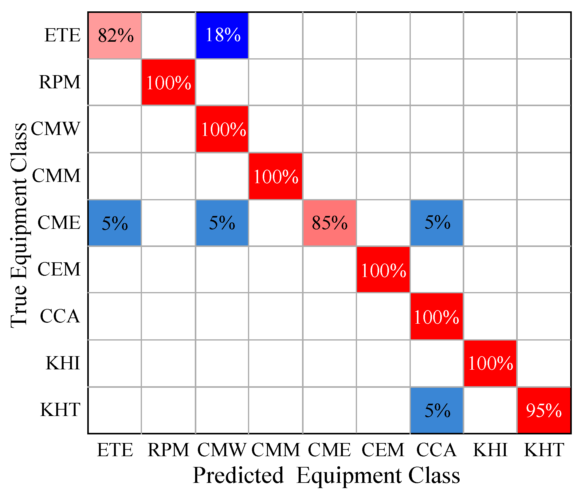
To evaluate the practicability of the proposed method in a realistic industrial scenario, the data from an actual Chinese cement plant were used in the experiments. Active power (P) and reactive power (Q) were collected at a sampling frequency of 1/300 Hz for each piece of equipment in the plant. The data were collected over the time span from September to November. Nine pieces of industrial equipment were selected for the study, and P and Q of the electrical equipment were used as input information. For 90 days of power data, the data were first divided by the basic time unit of 24 h. Then, the equipment power data were combined into data samples. Finally, the power dataset of the nine pieces of standard industrial electric equipment was formed. The authors abbreviated these nine units as follows: exhaust gas treatment exhaust motor (ETE), roller press motor (RPM), coal mill wind motor (CMW), coal mill main motor (CMM), cement mill exhaust motor (CME), cement mill main motor (CEM), cement circulating air motor (CCA), kiln head induced air motor (KHI), and kiln tail high temperature air motor (KHT). Unlike the public dataset in residential power scenarios, the sampling frequency of industrial scenarios in reality is very low, which leads to poorer quality of raw power data and more difficult identification of power loads.

The experimental data in this paper were from a real plant, so they contained many abnormal values. These anomalous data may have come from equipment failures or human error. However, the raw power data served as a valid basis for the experiment, and the presence of anomalous values may have caused the experiment to seriously deviate from the real results. Therefore, the data should be cleaned and denoised before the experiment to improve the data quality. According to research on industrial equipment, the load profile of industrial equipment has the following characteristics: firstly, the overall load profile changes smoothly over time and usually does not change abruptly; secondly, the industrial load profile is related to the production planning, and the adjacent dates when the equipment works should have similar load patterns. Considering the above, this paper preprocessed the dataset by replacing abnormal values, filling in missing values, and removing invalid dates.

2.2. Introduction to the Joint Time-Frequency Entropy Feature

Feature extraction relies on the original sampled data, and it reduces the high redundancy of the data by creating relevant new features. Industrial power scenarios are sampled at low frequencies, and much harmonic information is lost in the dataset, but harmonic information is commonly used in power signal analysis. For this reason, it is imperative to extract valuable load features from alternative perspectives. Considering the complexity of the electrical power load and the quality of the actual samples collected, this paper introduced entropy value characteristics after extracting time-frequency domain characteristics and subsequently constructed the joint feature set.

2.2.1. Time-Frequency Domain Features

The time domain feature (TD) used in this paper consists of 16 time-domain statistics. These include unitary statistics and unitless statistics. The unitary statistics usually have an intuitive physical meaning and include mean value, maximum value, minimum value, root mean square, peak-to-peak value, standard deviation, mean amplitude, root mean square amplitude, skewness, and kurtosis. Unitless statistics are usually written as the product or ratio of two statistical units whose final units cancel each other, and include skewness metrics, kurtosis metrics, margin metrics, impulse metrics, peak metrics, and waveform metrics. The frequency domain features (FD) used in this paper consist of 13 frequency-domain statistics. These 13 features include the mean value, standard deviation, center of gravity, root mean square, mean value of spectral cliff, standard deviation of spectral cliff, skewness of spectral cliff, two main band position change indicators and four correlation statistics showing the concentration or dispersion of the frequency spectrum.

The frequencies required for the calculation are obtained by the fast Fourier transform, a fast algorithm that performs the discrete Fourier transform on a computer. In signal processing, the computation of the discrete Fourier transform has an important place. The discrete Fourier transform can achieve correlation, filtering, and spectral estimation of signals. The following defines a discrete-time signal $x\left(n\right)$ to continuous Fourier transform.

$$X\left(e^{j\omega }\right)=\sum _{n=0}^{N-1}x\left(n\right)e^{j\omega n}$$

(1)

Because it is a continuous function, it cannot be calculated on a computer. Therefore, we can discretely approximate the spectrum of $x\left(n\right)$ and then perform the spectrum analysis on the computer. The definition of a discrete signal $x\left(n\right),n=0,1,2,\cdots ,N-1$ to discrete Fourier transform, is provided as follows:

$$X\left(k\right)=\sum _{k=0}^{N-1}X\left(k\right)w_N^{-nk}$$

(2)

where $w_N={\mathrm{e}}^{\left(-j2\sigma /N\right)},n=0,1,2,\cdots ,N-1$. The inverse transformation of the defined transformation is as follows:

$$x\left(n\right)=\frac{{\displaystyle \sum _{k=0}^{N-1}}X\left(k\right)w_N^{-nk}}{N}$$

(3)

The discrete Fourier variation in matrix form is $X=A\cdot x$, where the transformation matrix $A$ is:

$$A=\left(\begin{array}{cccc}1& 1& \cdots & 1\\ 1& w_N^1& \cdots & w_N^{N-1}\\ ⋮& ⋮& \ddots & ⋮\\ 1& w_N^{N-1}& \cdots & w_N^{{\left(N-1\right)}^2}\end{array}\right)$$

(4)

2.2.2. Entropy Value Feature

The subset of entropy value feature (EV) used in this paper consists of seven entropy calculations, including permutation entropy, fuzzy entropy, sample entropy, approximate entropy, energy entropy, singular spectrum entropy, and power spectrum entropy. Entropy describes the system chaos, which can be used to describe the state change of industrial power equipment. A lower entropy value reflects reduced ambiguity in the information, which means less chaos. The entropy of a system can be defined as follows.

Suppose that $M$ is a $Lebesgue$-space, possessing $\mu$-measure, and $\mu \left(M\right)$ equals 1. Use the incompatible finite partition $A=\left\{A_i\right\}$ to describe $M$. $M={\displaystyle {\sum }_{i=1}^N{A}_i}$ and $A_i\cap A_j=\mathsf{\Phi }$, $\forall i\ne j$. The entropy for the partition of $A$ is defined as:

$$H\left(A\right)=-A\mu \left(A_i\right)\log \mu \left(A_i\right)$$

(5)

where the metric of the set $A_i$ is $\mu \left(A_i\right)\left(i=1,2,\cdots ,N\right)$.

2.3. Introduction to the EO Principle

A recently developed physical optimization algorithm named equilibrium optimizer can be applied to resolve continuous optimization problems. The candidate particles in the EO algorithm are the sum of the four best particles and their arithmetic mean, which is analogous to the highest-rated triad of wolves in the grey wolf optimization algorithm (GWO). The above four candidate particle combinations contribute to the effectiveness of the EO algorithm. Equilibrium candidate groups construct their equilibrium pool.

$$C_{ave}=\frac{\left(C_{eq1}+C_{eq2}+C_{eq3}+C_{eq4}\right)}{4}$$

(6)

$$C_{eq,pool}=\left\{C_{eq1},C_{eq2},C_{eq3},C_{eq4},C_{eq\left(ave\right)}\right\}$$

(7)

The exponential factor $\left(F\right)$ regulates the algorithm’s plausible equilibrium during the particle update.

$$F=a_{1}sign\left(r-0.5\right)\left[e^{-\lambda t}-1\right]$$

(8)

$$t={\left(1-\frac{Iter}{Max\_iter}\right)}^{\left(a_2\frac{Iter}{Max\_iter}\right)}$$

(9)

Here, $\lambda$ and $r$ are two vectors of random values within the range [0, 1], and t decreases as the number of iterations increases. The parameters $Iter$ and $Max\_iter$ refer to the present and maximum iteration number for the particle, respectively, for better population diversity and guaranteed convergence. $a_2$ denotes the exploration capacity constant; the exploration aptitude is greater and the exploitation aptitude is lower when $a_2$ is higher. The values of $a_1$ and $a_2$ can be modulated at any point as per the requirements of the particular algorithm. As the EO algorithm, a fundamental factor affecting the developmental stage is the generation rate G, and its model is specified as:

$$G=G_{0}F$$

(10)

$$\overrightarrow{G_0}=\overrightarrow{GCP}\left(\overrightarrow{C_{eq}}-\lambda C\right)$$

(11)

$$\overrightarrow{GCP}=\{\begin{array}{l}0.5r_1 r_2\ge GP\\ 0 r_2\le GP\end{array}$$

(12)

The algorithm’s mining and exploration capacity is demonstrated in Equation (10). If the signs of $G_0$ and $F$ are identical, the mining capacity is greater, and if opposite signs are employed, the exploration capacity is heightened. $GP$ determines the effect of $G_0$ on $G$. When $GP$ is 1, Equation (11) does not hold. $G$ is applied to manage the rapid accumulation of solution volume, with $G_0$ representing the concentration at the start; both $r_1$ and $r_2$ refer to vectors of random numbers within the range of [0, 1]. In Equation (12), $GCP$ indicates the potential of particle renewal generating rate $G$, with the renewal process being more effective when $GCP$ is 0.5. The final equation of particle renewal is described as:

$$C=C_{eq}+\left(C-C_{eq}\right)F+\frac{G}{\lambda V}\left(1-F\right)$$

(13)

In the context of the EO algorithm, each particle and its position are viewed as a search state. At each cycle, a search state’s present position is updated randomly based on the equilibrium candidate. In Equation (13), the first segment denotes the equilibrium position, while the second portion $C$ and $C_{eq}$ represent the present particle and the equilibrium candidate separately. The position deviation between these two indicates proximity to the global optimal particle, which enlarges the search scope and enhances population diversity. The last portion leads to better exploitation and reduced likelihood of local optimum occurrence.

2.4. EO for Feature Selection

Feature selection constructs a low-dimensional features subset, but retains the complete information expressed by the overall features. The advantages are improved experimental accuracy, reduced feature dimensionality, and reduced model time cost. As a metaheuristic algorithm, the EO is used in feature selection as a wrapper-based optimization search strategy. However, feature selection is an optimization issue that involves discrete values of 0 or 1 for particle concentration. Therefore, a binarization operation is required.

2.4.1. Binary Operation

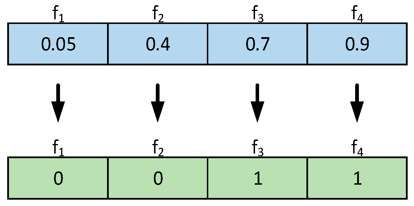
For the EO in continuous cases, particles can be located at any position density. For discrete cases, to maintain conversion effectiveness of the continuous algorithm to binary, the following function is applied to complete such conversion.

$$C_{ij}^{iter+1}=\{\begin{array}{l}1 if C_{ij}^{iter+1}>\sigma \\ 0 otherwise\end{array} j=1,\cdots ,D$$

(14)

In this function, $\sigma \in [0,1]$ represents a random variable. If $C_{ij}^{iter+1}$ exceeds this random variable, the continuous value is converted to “1”, signifying that the corresponding feature is chosen during classification. If $C_{ij}^{iter+1}$ is smaller than this value, the continuous value is changed to “0”, indicating that the corresponding feature is excluded.

To visually represent the dualization results, the authors show the dualization results of $\sigma =0.5$ in Figure 2.

In Figure 2, f₃, f₄ are selected by the algorithm because they correspond to a value of 1 after binarization.

2.4.2. Fitness Function

The objective of EO feature selection is to maximize relevance and minimize redundancy, and to obtain optimal results. Therefore, KNN is used as the classifier algorithm, and the classification error rate of electric load identification is used as the fitness function:

$$Fitness=1-Accurac{y}_{test}$$

(15)

where, $Accurac{y}_{test}$ is the experimental accuracy of the test set.

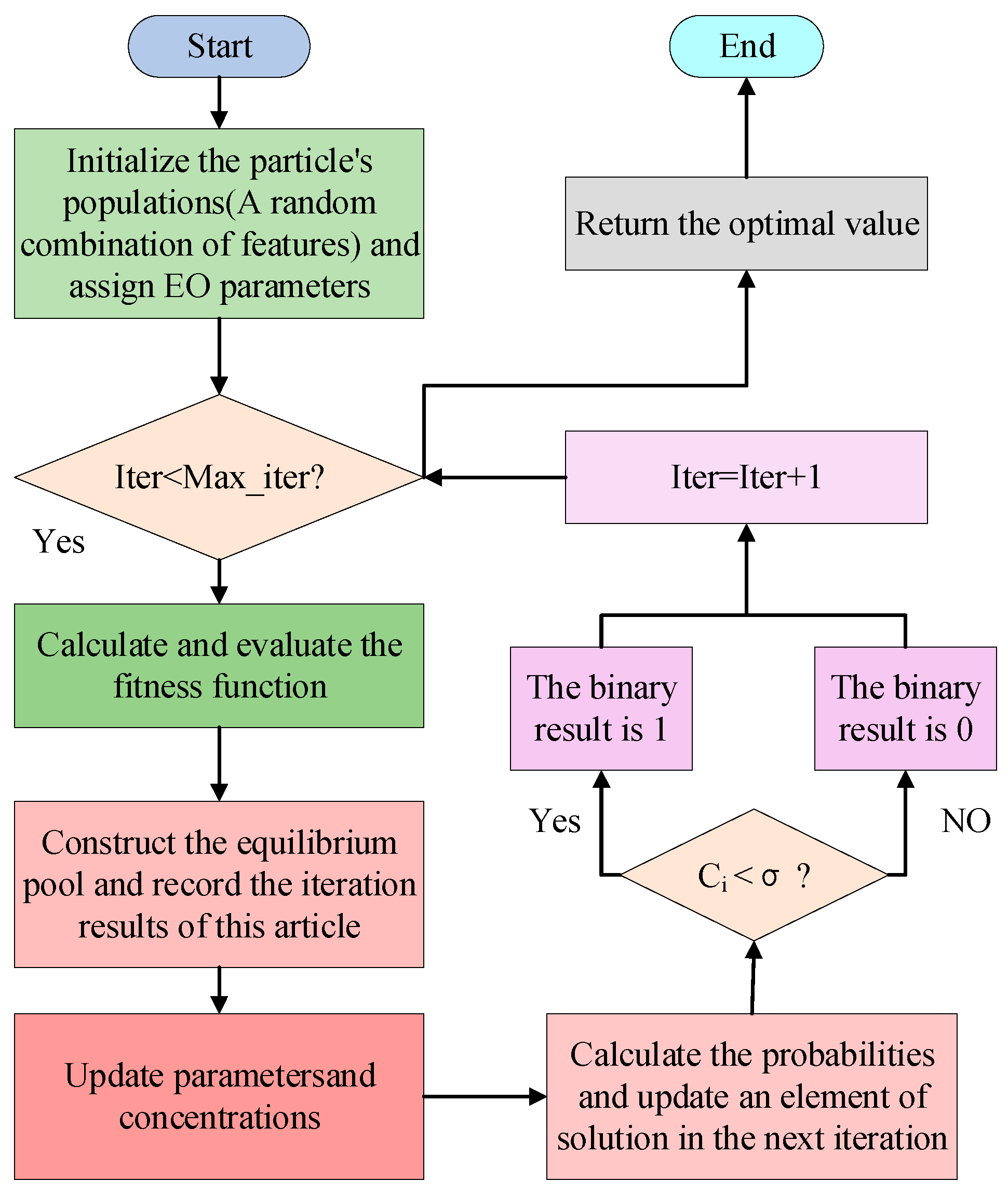
Figure 3 demonstrates the process flow of the EO for feature selection.

3. Experiments and Analysis of Results

3.1. Data Presentation

In this paper, nine standard pieces of industrial equipment from a Chinese cement plant were selected as experimental subjects, and the original dataset included three months of electrical measurement parameters of the equipment. Due to the low sampling frequency of industrial power scenarios, the quality of raw power data is poor. Therefore, the authors improved the data quality by pre-processing data cleaning and denoising to reflect the actual identification results. To visualize the data processing, the authors selected reactive and active power of KHT to reflect alterations in the power curve, as shown in Figure 4. Each curve in Figure 4 shows the load changes for 24 h of the day. Among them, (a) shows the active power curve for 90 days before KHT pre-processing, and (b) shows the reactive power curve for 90 days before KHT pre-processing. (c) shows the active power curve for 72 days after KHT pretreatment, and (d) shows the reactive power curve for 72 days after KHT pretreatment.

Firstly, observe the original power curve before preprocessing. The active power before preprocessing spans an extensive range of adjacent dates with obvious outliers, which cannot reflect the fundamental operation law of the equipment. The main reason is that the raw power data contain many abnormal and outlier values. Furthermore, when the data are contaminated with outliers, the trained model parameters are misdirected, and the model cannot accurately analyze the equipment type. Subsequently, the active power after preprocessing is observed. Comparing the power curves before preprocessing, the preprocessed industrial dataset eliminates outliers, the power levels are more aggregated, and the equipment operation patterns are apparent. Interestingly, the authors found that active and reactive power load curve patterns were very similar after preprocessing. However, the power levels were very different, reflecting the industrial equipment’s uniqueness. By cleaning the raw power data and denoising them, the data quality of the power load is improved. This is a prerequisite for subsequent feature processing and model training.

3.2. Extraction of Entropy Value, Time Domain, and Frequency Domain Features

Due to the multiple limitations of the acquisition scenario and sampling conditions, the raw power samples suffered from severe data redundancy and high data dimensionality. Feature extraction can decrease data complexity and computation time of the model, while improving the classifier’s performance. For the data type of industrial power loads, the classical time-frequency domain features have problems such as high complexity and insufficient accuracy. To prevent the loss of important information from the original power data during feature conversion, the authors introduced entropy value features after extracting time-frequency domain features.

Based on the feature principle, the authors extracted 72 dimensional features from the raw power data and aggregated them into a joint feature set. These included 14 dimensional entropy value features (7 dimensional active power and 7 dimensional reactive power), 32 dimensional time-domain features (16 dimensional active power and 16 dimensional reactive power), and 26 dimensional frequency-domain features (13 dimensional active power and 13 dimensional reactive power) of the power load.

3.3. EO Screening Joint Features

Feature selection is an essential process for any classification task, which finds the subset of features with the smallest dimensionality by retaining the primary information carried by all features. In feature selection, the metaheuristic algorithm is used as a wrapper-based feature selection method, which has proven superiority in reducing the training time and improving model accuracy. The metaheuristic algorithm EO is used to screen the joint features to obtain a subset of features suitable for identification. Feature selection outcomes are presented in

Table 1. Feature locations and ratios for EO screening.

Type	Feature Type	Feature Number	Screened Features Number	Proportion
Active power	TD	1–16	3, 11, 13	19%
	FD	17–29	19, 28	15%
	EV	30–36	30, 31, 33, 34	57%
Reactive power	TD	37–52	37, 38, 46	19%
	FD	53–65	53, 56, 58, 62, 64	38%
	EV	66–72	66, 67, 68, 72	57%

To clarify the feature locations, the features of active power are ordered as time domain (1–16), frequency domain (17–29), and entropy value (30–36). The features of reactive power are ordered as time domain (37–52), frequency domain (53–65), and entropy value (66–72).

. According to this table, EO screens nine active power load features and 12 reactive power load features. The dimensionality of the features selected by EO is 29% of the joint feature set (filtering out 21 dimensions from 72). Among them, the entropy value features are more distributed in the subset of screened features, and 57% of the feature proportion is screened in active power and reactive power, respectively. The time-frequency domain exhibits a lower screening ratio. The findings demonstrate that entropy value features make the most significant contribution to the combined feature set. Using EO feature selection in industrial power scenarios can significantly reduce the dimensionality of the joint features.

Because the distribution of features reflects the inherent structure and patterns of the data, the visualization of feature distribution is an essential component of the feature selection and classification process. In Figure 5, box and whisker plots can identify anomalies among the 21 selected features, provide the data distribution for each feature, and allow for their comparison. The mean of the texture is represented by the horizontal line in the frame at the bottom. The first horizontal line represents the first quartile of the average texture. The second horizontal line indicates the texture median. The horizontal line at the top of the graph represents the utmost value of the texture’s mean, and the tiny diamonds are outliers. Due to their feature types and data quality, the distribution of the screened features has some variability. There are a few anomalies, among which the feature extraction values of the entropy-valued features are generally lower and more densely distributed.

3.4. Classification of Different Models

To test the effectiveness of EO feature selection in industrial electricity scenarios, the experiments used a subset of EO-screened features as model input and trained KNN, SVM, DT, RF, DA as classifiers, respectively. The authors introduced 10-fold cross-validation to enhance the reliability and effectiveness of various classification models. The samples were randomly divided according to 70% training set and 30% test set, and five independent experiments were used to equalize the results.

Table 2. Classifier parameters.

Classifier	Core Parameter	Description
KNN	K = 5, Dmetric = Euclidean:	K denotes nearest neighbor number in input data used to classify each point, and Dmetric distance metric for the KNN algorithm.
SVM	Kernel = ‘rbf’, C = 2:	“rbf” stands for radial basis function for kernel function selection, C represents penalty parameter.
DT	DTmax = 20:	DTmax indicates the maximum number of decision splits or branch nodes that can exist in each tree.
RF	RFtree = 25, FEmax = 10:	RFtree means the number of trees in the forest, FEmax indicates the setting of the maximum number of features.
DA	DE = ‘linear’, S = 0.2:	DE is the discriminant function, “linear” means linear discriminant, S indicates the setting of the smoothing parameter.

presents information regarding the parameters of the basic classifier.

The first concern is the accuracy. In

Table 3. Accuracy of electric load identification.

Classifier	Test1	Test2	Test3	Test4	Test5	Mean Value	Standard Deviation
KNN	93.37%	91.05%	96.21%	95.73%	92.43%	93.76%	1.96%
SVM	95.88%	95.23%	95.50%	94.71%	96.56%	95.58%	0.62%
DT	95.68%	96.07%	95.11%	95.24%	91.02%	94.62%	1.83%
RF	96.76%	95.34%	95.28%	96.39%	92.03%	95.16%	1.67%
DA	92.75%	94.73%	90.69%	92.38%	92.61%	92.63%	1.28%

, the mean value and standard deviation of accuracy from multiple experiments were calculated. Table 3 shows that all of the features screened by EO had an accuracy of more than 92% in electric load identification. Among them, the average accuracy of SVM was higher than that of the rest of the classifiers, reaching 95.58%. The average accuracy of DA was the lowest, but it also reached 92.63%. Additionally, the authors found that the stability of SVM was higher than that of the other classifiers in the experiment, with a standard deviation of 0.62%. The main reason why SVM provided the lowest classification stability while ensuring optimal classification was that it is more suitable for processing low-frequency power signals.

To demonstrate the practical effectiveness of the method proposed in this paper for identifying electrical loads in industrial settings, visualizations were created. In Figure 6, the confusion matrix demonstrates the classification details of the electrical loads for SVM. From Figure 6, the identification of each industrial piece of equipment can be clearly understood. The blue color indicates incorrect classification and the red color indicates correct classification. Among them, 82% of the equipment type ETE was correctly identified and 18% was incorrectly identified as CMW. Additionally, 85% of the equipment type CME was correctly identified, while 5% was incorrectly identified as ETE, 5% was incorrectly identified as CMW, and 5% was incorrectly identified as CCA. Further, 95% of the equipment type KHT was correctly identified and 5% was incorrectly identified as CCA. All of the rest of the equipment was correctly identified. Therefore, the features screened by EO from the joint features can help the model analyze the industrial equipment types accurately.

EO feature selection is feasible in terms of the accuracy of electric load identification. Figure 7 shows the computation time of the model. From Figure 7, the computation time of EO-screened features in electric load identification was less than 8 s. The time cost of different classifiers varied significantly, among which SVM had the most stable computation time with an average computation time of 0.75 s. For industrial power scenarios, EO-screened features are more efficient regarding model computation time. In conclusion, the approach introduced in this paper can achieve precise electrical load classification and requires minimal computation time. The proposed method is both practical and feasible in real-world industrial power settings.

4. Comparison Experiments

4.1. Comparison before and after Feature Extraction

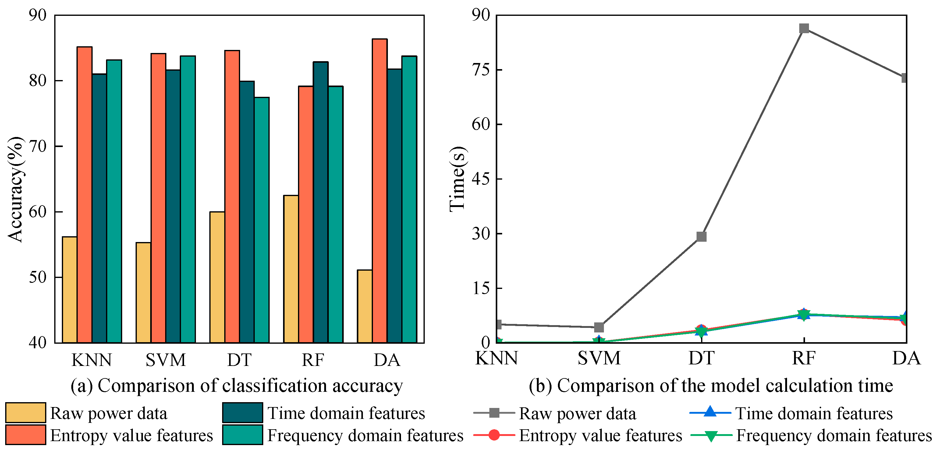
To demonstrate the necessity of feature extraction in industrial power scenarios, experiments were compared using raw power data and three independent feature sets (after feature extraction). KNN, SVM, DT, RF, and DA were chosen as the base classifiers in the experiments, and different data types were used as model inputs. The authors introduced 10-fold cross-validation to enhance the reliability and effectiveness of various classification models. The classification accuracy and computation time for nine pieces of industrial equipment are shown in Figure 8. As illustrated in Figure 8, the left panel exhibits a comparison of classification accuracy between the original power data and three independent features, while the right panel compares the computational time of the models.

Firstly, observe the comparison of the accuracy before and after feature extraction. The raw power data were poor on different classifiers, where the classifier with the highest accuracy was RF with 62.5%. The classifier with the worst classification accuracy was DA, which was only 51.12%. For industrial power scenarios, raw power data cannot meet the usage requirements in terms of accuracy. The three load features extracted from the raw power data improved the effect on the classifier significantly. Among them, entropy features exhibited a higher classification accuracy in comparison to time domain and frequency domain features. Taking SVM as an example, the classification accuracy of the entropy value feature reached 84.17%, which was 52.18% better than that of the raw power data. Subsequently, focus on the change in model computation time before and after feature extraction. The difference in raw power data was more evident in different classification models. Among them, SVM had the shortest computation time of 4.2412 s. In contrast, RF had the longest computation time, which reached 86.3788 s. The main reason for such an extended model computation time for raw power data was the high dimensionality of the data and the complexity of the model computation. After extracting the features, the time cost of the model was greatly reduced. Among them, the computation time for the three independent feature sets was relatively similar. Taking SVM as an example, the computation time for the entropy value feature model was only 0.1353 s, which was 3.19% that of the initial power dataset. Moreover, computation time for time domain features and frequency domain features also declined, to 0.1697 s and 0.1644 s, respectively. Due to the variability of classifiers, the time reduction for RF was the most obvious, and the computation time for entropy value features was reduced by 78.5805 s after feature extraction. With feature extraction, the model input dimensionality of industrial equipment was reduced from 288 to 14 dimensions (entropy value features). The remarkable decrease in dimensionality truly minimized the model computation time and simultaneously enhanced recognition accuracy. Thus, feature extraction not only preserves the information relevance of the industrial equipment, but also greatly reduces the redundancy of the data.

4.2. Feature Combination Comparison

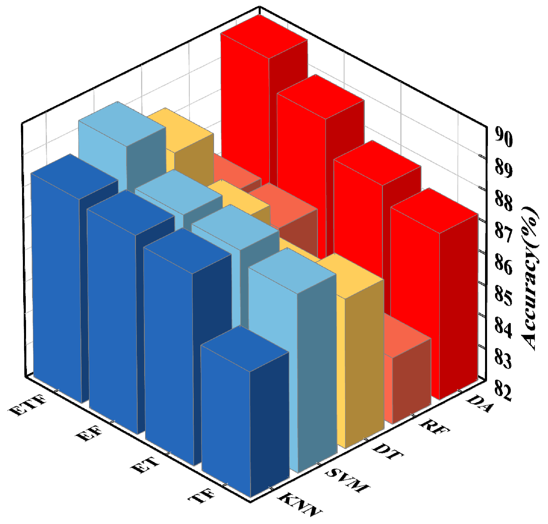
A wealth of feature extraction space is essential for model performance improvement. To expand the feature space, numerous features were obtained from the raw data, and an attempt was made to combine them. To compare the pros and cons of different feature combinations in identifying electricity consumption in industrial power scenarios, the authors developed identification models using different classifiers and used the recognition accuracy of the corresponding classifiers as the judging criteria. The feature combinations were used as model inputs. Their accuracy comparisons on different classifiers are presented in bar charts, as in Figure 9. The combinations of two features included time domain features with frequency domain features (abbreviated as TF), entropy value features with time domain features (ET), and entropy value features with frequency domain features (EF). There was also a joint feature set (ETF) that aggregated all features.

Observing the effectiveness of feature combinations for identifying electrical loads, the authors found variability in the accuracy of different classifiers. Among them, the highest classification accuracy was achieved using the joint feature set, which is very intuitive, with 88.44%, 89.35%, 88.41%, 88.25%, and 89.89% on KNN, SVM, DT, RF, and DA, respectively. SVM was employed as an exemplification to examine the accuracy of various models with varying feature combinations. First, in comparing the two feature combinations, EF had the best accuracy rate of 88.17%, ET gave the next best result, of 88.03%, and TF had the worst result, of 87.64%. Subsequently, ETF had the best result, with an accuracy of 89.35%. Interestingly, the accuracy of feature combinations that included entropy features was usually higher. The results show that combining features is beneficial to exploit the advantages of multiple features jointly. Entropy value features contribute the most to the joint feature set, and introducing entropy value features can improve the overall feature quality.

4.3. Comparison of Feature Selection Methods

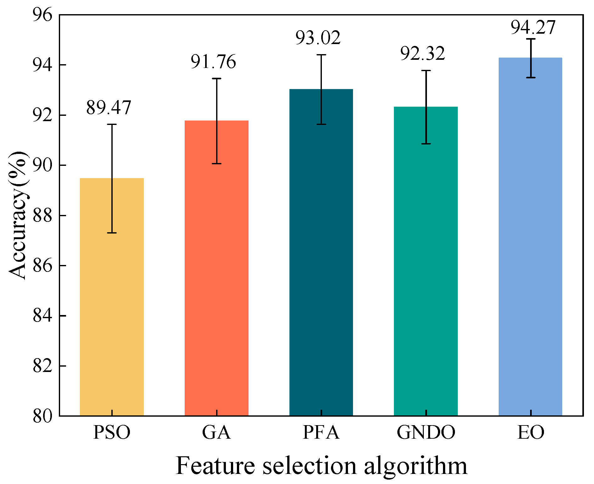
Feature selection finds the subset of features with the smallest dimensionality by retaining the primary information carried by all features. Four metaheuristic feature selection methods were selected for comparison to reflect the algorithmic quality of the EO. These included the classical particle swarm optimization (PSO) and genetic algorithm (GA), as well as the recently proposed pathfinder algorithm (PFA) and generalized normal distribution optimization (GNDO). Since comparing algorithms is a stochastic technique, a fair comparison using the same parameters is required. Experiments were carried out to confirm the effectiveness of feature selection on KNN using the joint feature set as the model input. The authors introduced 10-fold cross-validation to enhance the reliability and effectiveness of various classification models. Five independent repeat experiments were performed to test the stability.

First, observe the algorithm’s accuracy. Using a bar chart to depict the average accuracy and an error bar to indicate standard deviation, Figure 10 visually illustrates the comparison of the precision from different feature selection algorithms. As indicated in Figure 10, the accuracy of the features screened by the EO was higher than that of the remaining four algorithms, with an average accuracy of 94.27%. The accuracy of the other four algorithms ranged from 89.47% to 93.02%. The authors also noted that the EO had the best stability in screening features, with the lowest standard deviation of 0.7718%. Thus, the EO has an advantage over the classical (PSO, GA) methods in terms of accuracy and also over the algorithms newly proposed in recent years (PFA, GNDO).

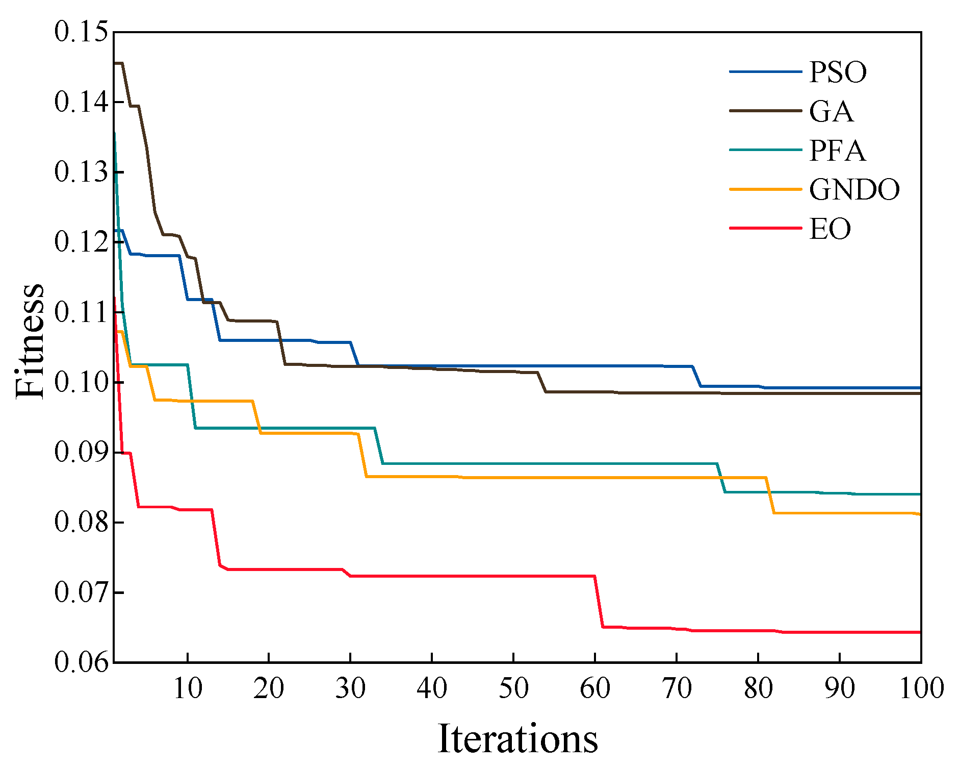
After comparing the accuracy, the focus was on the feature dimension of the screening. The convergence curve of the feature selection process was observed through 100 iterations. During the iterations, the error rate was adopted as the fitness function. The iterations are shown in Figure 11. The EO reduced the error rate from 0.11203 to 0.06431 after 83 iterations. The EO had the best adaptation compared to PSO, GA, PFA, and GNDO, indicating that it has better feature selection ability for industrial power loads. After completing the iterations, the feature selection dimensions of the different algorithms were recorded. Among them, the EO had 21 dimensions, the PSO had 35 dimensions, the GA had 32 dimensions, the PFA had 34 dimensions, and the GNDO had 29 dimensions. The EO had a minor feature dimension, and a smaller feature dimension will also make the feature subset more efficient in terms of time cost.

Therefore, the feature subset screened by the EO was optimal for the joint feature set, with the EO able to completely account for the relevance and redundancy when filtering features. It retained the primary information of the joint feature set and filtered out irrelevant information. Irrelevant information is often the cause of data analysis and model complexity. Interestingly, the authors also found that the feature attributes screened by different algorithms were more similar, with entropy value features having the highest probability of being selected. This indicated that the entropy value features contained richer information about the industrial equipment and were more effective for electric load identification. Therefore, the introduction of entropy value features and the use of the EO to screen features are efficient. The method described in this paper can be an excellent solution to the electric load identification problem in industrial power consumption scenarios.

5. Conclusions

Electric load identification in industrial power consumption scenarios can optimize power consumption structure and improve power consumption efficiency, which is a prerequisite for intelligent energy management. The sampling environment of the industrial electricity consumption scenario is harsh, and the sample quality is poor. Therefore, how useful features are extracted from the low-frequency data and appropriate feature combinations are screened out from the joint feature set determines the effectiveness of equipment identification. To solve this problem, this paper proposed an EO-based feature selection method to screen the time-frequency entropy joint feature set in industrial electricity scenarios. This study offers the following key contributions:

• Solved the problem of power load identification using low-frequency data in industrial power scenarios. The experiments used active and reactive power signals with a sampling frequency of only 1/300 Hz to accurately classify nine typical industrial equipment types.
• Introduced entropy value features on the basis of time-frequency domain features and constructing joint feature sets. Taking SVM as an example, compared with the original power data classification effect, the extraction of entropy value features improved accuracy by 61.31%. At the same time, the computation time for the model was reduced to 0.1353 s. The construction of the joint feature set further improved the classification accuracy of power equipment to 89.35%, in which the entropy value features contributed the most to the entire feature set.
• Used EO to screen the joint features of electric loads to obtain the best feature subset. The EO reduced the joint feature dimensionality from 72 to 21 dimensions. In power load identification, the 21 features screened by the EO improved the classification accuracy of devices to a maximum of 95.58% and reduced the time cost to a minimum of 0.045 s. Thus, the EO balanced the relevance and redundancy of feature screening and achieved the goal of filtering out invalid data while ensuring information integrity.

In summary, in the problem of electric load identification in industrial power consumption scenarios, this paper was very effective in introducing entropy value features after extracting the time-frequency domain and using an EO to screen the joint features, which provides a basis for subsequent industrial energy optimization and intelligent energy management. In future research, the research process of this paper can be used as a template for task implementation, and the problems of long training times, memory limitations, and low data quality can be solved by combining multiple features with novel and effective feature selection methods to cope with the redundancy caused by massive data in general application scenarios.

There were some limitations and areas for improvement in the current research content of this paper. Firstly, in terms of data types, there were limitations and differences in different feature extraction means for various types of signals and datasets. The quality of time and frequency domain features extracted from industrial power data in this paper must be improved. How to extract suitable features for data types will be the focus of the authors’ work in the future. Secondly, in terms of application scenarios, the identification scenario in this paper was industrial, while commercial electricity consumption has also been greatly enhanced in recent years, so the results of this paper may have some limitations. To solve this problem, the authors will conduct joint research on multiple scenarios in the future.