Article

Efficient Dynamic Deployment of Simulation Tasks in Collaborative Cloud and Edge Environments

College of Systems Engineering, National University of Defense Technology, Changsha 410073, China
*
Author to whom correspondence should be addressed.
Appl. Sci. 2022, 12(3), 1646; https://doi.org/10.3390/app12031646
Submission received: 25 November 2021 / Revised: 30 January 2022 / Accepted: 30 January 2022 / Published: 4 February 2022

Abstract

:
Cloud computing has been studied and used extensively in many scenarios for its nearly unlimited resources and X as a service model. To reduce the latency for accessing the remote cloud data centers, small data centers or cloudlets are deployed near end-users, which is also called edge computing. In this paper, we mainly focus on the efficient scheduling of distributed simulation tasks in collaborative cloud and edge environments. Since simulation tasks are usually tightly coupled with each other by sending many messages and the status of tasks and hosts may also change frequently, it is essentially a dynamic bin-packing problem. Unfortunately, popular methods, such as meta-heuristics, and accurate algorithms are time-consuming and cannot deal with the dynamic changes of tasks and hosts efficiently. In this paper, we present Pool, an incremental flow-based scheduler, to minimize the overall communication cost of all tasks in a reasonable time span with the consideration of migration cost of task. After formulating such a scheduling problem as a min-cost max-flow (MCMF) problem, incremental MCMF algorithms are adopted to accelerate the procedure of calculating an optimal flow and heuristic scheduling algorithm, with the awareness of task migration cost, designed to assign tasks. Simulation experiments on Alibaba cluster trace show that Pool can schedule all of the tasks efficiently and is almost 5.8 times faster than the baseline method when few tasks and hosts change in the small problem scale.

1. Introduction

By incorporating grid computing, virtualization technology, and the idea of servitization, cloud computing, as a new computational paradigm, has been widely studied and applied in many fields since its emergence. The most influential definition of cloud computing is given by National Institute of Standards and Technology (NIST) [1], who firstly proposed three service models: Infrastructure as a Service (IaaS), Platform as a Service (PaaS), and Software as a Service (SaaS), and four deployment patterns, namely public cloud, private cloud, community cloud, and hybrid cloud [2]. The main advantages of cloud computing can be summarized as serve-as-you-need, widely network access, elastic scaling, and efficient management.
Computer simulation, as a kind of computer application, has been used widely, such as education, entertainment, medical care, and military field. However, with the deepening and extension of its application, simulation also confronts many new issues [3]. On the one hand, the increasing number of simulation entities and the continuously refined model functions call for more computing resources. Simulation users need to pay a great amount of money to buy, operate, and manage these high-performance servers. On the other hand, the heterogeneous simulation models, systems, and other simulation resources developed by different institutes are isolated with each other, which may result in repeated development and waste of resources.
Considering the issues associated with simulation and the advantages of cloud computing, a new research area called cloud-based simulation or cloud simulation comes into being [3,4,5]. Fujimoto et al. [3] summarized the benefits of combining simulation and cloud technology from four aspects: (1) reducing the usage cost of simulation; (2) simplifying the usage of simulation; (3) helping the operation and management of simulation resources; (4) improving the capacity of fault tolerance.
Although cloud computing can bring many benefits to simulations, some limitations also exist. For example, cloud data centers are usually located far away from users, which may incur long data transmission delay. As some simulation applications, especially those involved with real human or equipment, are sensitive to the time delay, edge computing [6] is introduced as a compliment for cloud computing.
Unlike the relatively independent tasks submitted by common users, simulation tasks tend to be tightly coupled. At the same time, they are usually highly heterogeneous and both communication-sensitive and computation-sensitive [7]. To achieve the high performance of executing simulations in the cloud, we need to assign all the tasks to proper hosts in a reasonable time span. In this paper, we mainly focus on the efficient task scheduling of simulation tasks in collaborative cloud and edge environments. Considering the frequent changes of the status of tasks and hosts, it is actually an NP-hard dynamic bin-packing problem.
Many scholars have conducted in-depth research in this field and put forward many useful solutions. To achieve the fast responses to users’ requests, task schedulers, which have been seen as the core modules in modern clusters, are needed to assign the submitted tasks to hosts efficiently. From the perspective of the working mechanism, they can be classified as queue-based [8,9,10] and batching-based schedulers [11,12,13]. In queue-based schedulers, tasks are assigned sequentially according to some predefined rules. To cope with a great number of tasks, these queue-based schedulers can be further divided as centralized, distributed, and hybrid designs. As tasks are processed independently, this kind of schedulers can be easily implemented in a parallel or distributed manner and can be deployed on-line without the need of a priori knowledge about tasks. On the contrary, batching-based schedulers try to deploy tasks jointly aimed at finding the global optimal assignment decision. As all the information about tasks and hosts is needed, this kind of scheduler requires more a priori knowledge and usually more time is consumed to solve such a combinational optimization problem. Considering the frequent message transmissions between simulation tasks, they should be deployed jointly to avoid degrading the performance of simulation applications. Thus, scheduling simulation tasks with a batching-based scheduler is a better choice.
To solve such an NP-hard problem, many algorithms are also proposed. Some researchers adopted meta-heuristics to find approximate optimal solutions. These algorithms are usually inspired by natural phenomena [14], such as the predation behaviors of birds (particle swarm optimization, PSO) and ants (ant colony optimization, ACO). Although they are easy to perform well in some optimization problems with complicated constraints, they tend to be time-consuming and non-deterministic even if all the parameters keep unchanged. To improve the time performance of the scheduler, heuristics were also utilized by some scholars, such as dominant resource fairness [15] and shortest job first [16]. As a trade-off, the deployment quality of tasks is not always satisfying and it is prone to fall into local minimum for these algorithms.
By relaxing some constraints and converting the task scheduling problem into a min-cost max-flow problem, tasks can be scheduled jointly in polynomial time, which is called flow-based scheduling [17,18,19]. In this method, tasks and computation nodes are modeled as nodes and the feasible deployment solutions are modeled as arcs. By setting the cost value and upper capacity of each arc properly, the final assignment decisions can be extracted from the generated optimal flow. However, current flow-based schedulers cannot deploy tasks efficiently, especially when the status of tasks and hosts changes frequently. In this paper, we propose a new scheduler called Pool to cope with this issue. Firstly, the network optimization problem is solved efficiently using incremental MCMF algorithms in Pool. Then, tasks are rescheduled with the consideration of migration cost of tasks. In such a way, tasks are deployed properly with the aim of minimizing the communication cost of all tasks, as well as reducing the overall migration cost when the status of tasks and hosts changes. Compared to the existing flow-based schedulers, Pool can achieve almost 5.8 times faster time performance with a small proportion of changing tasks and hosts.
In summary, the main contributions of this paper can be stated as follows:
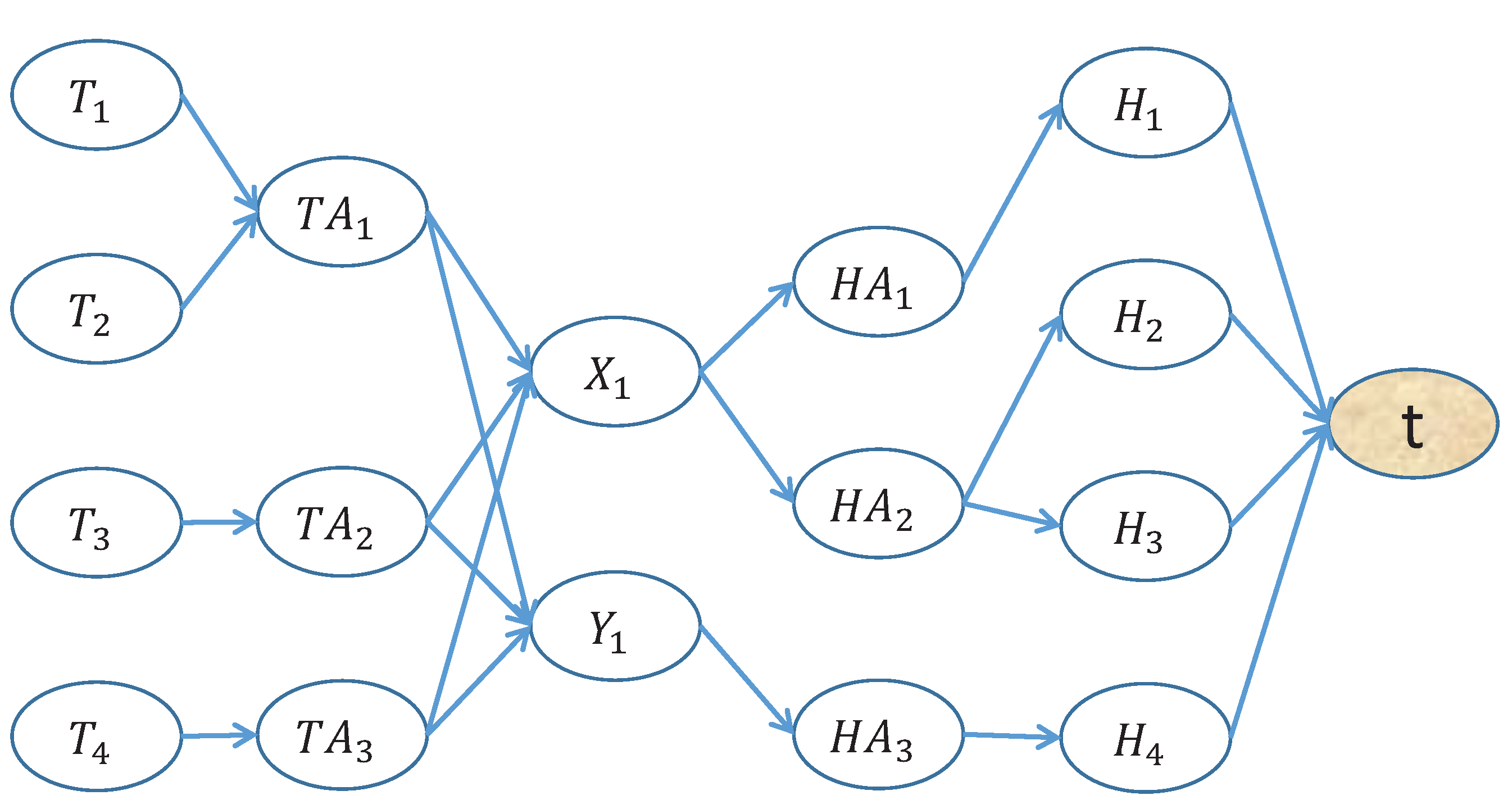
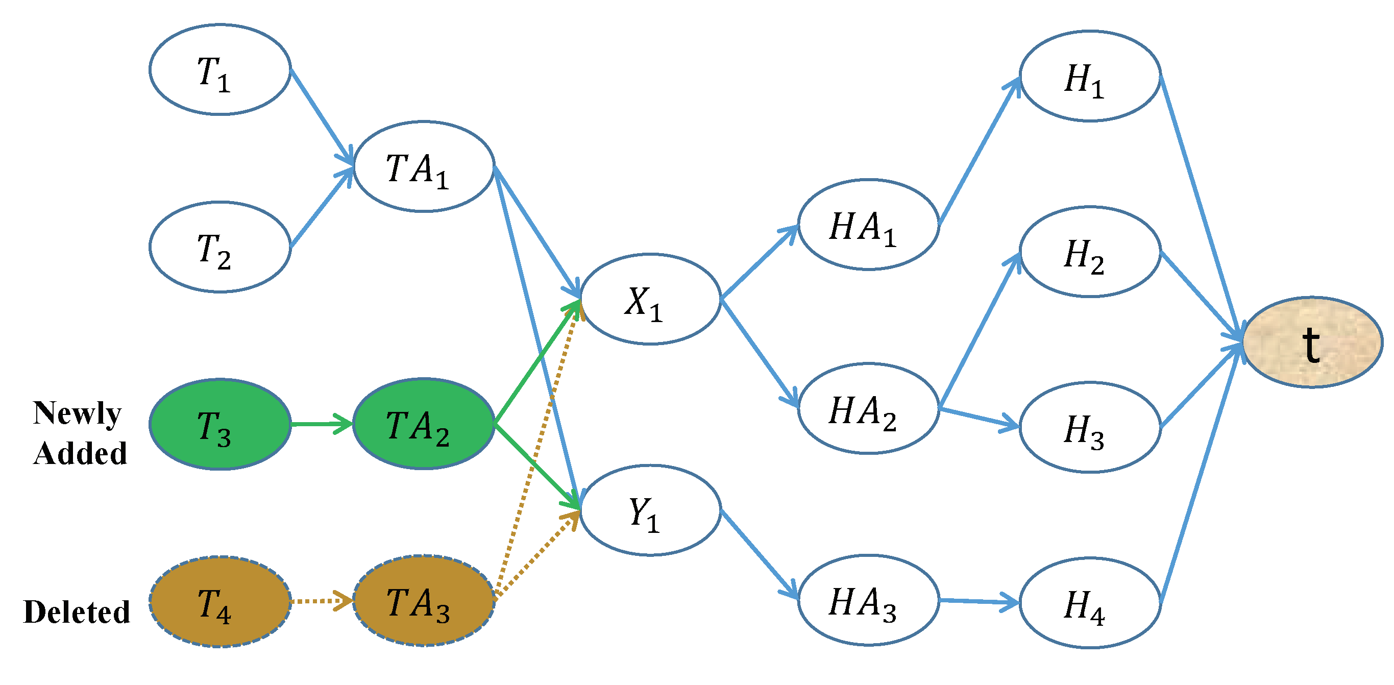
  • We formulate the problem of scheduling simulation tasks in collaborative cloud and edge environments as a MCMF problem and incremental MCMF algorithms are adopted to find the optimal flow quickly when the status of tasks and hosts changes;
  • We propose a new heuristic method to reschedule tasks efficiently based on both the newly generated optimal flow and the current deployment decisions of all tasks to minimize both the overall communication cost and the migration cost of all tasks;
  • Extensive experiments on Alibaba cluster trace are conducted to illustrate the effectiveness of Pool.
The rest of this paper is organized as follows: Section 2 reviews the related work about task scheduling. Section 3 states the problem background and models it as a MCMF problem. Section 4 details the design of our incremental task scheduler. Section 5 evaluates the performance of Pool, and conclusions and possibilities of future works are given in Section 6.

2. Related Works

Task scheduler is a very import module in current clusters and there are many impressive achievements in this area. In this section, the current research work is summarized in detail from two perspectives, namely scheduler structures and scheduling algorithms.

2.1. Scheduler Structures

According to the structure of schedulers, they can be centralized, distributed, and hybrid. In centralized designs, all the information about tasks and hosts is collected by the centralized scheduler and each task is processed based on global information. A single scheduler is adopted in Borg [8] to improve the resource utilization with the consideration of machine sharing and performance isolation. Jin et al. [20] proposed a task execution framework called Ursa, in which a centralized task scheduler was adopted to assign tasks globally. Although better deployment quality can be obtained, the deployment latency may increase since information about all tasks and hosts needs to be collected, especially when the number of tasks is very large.
To deal with a high throughput of tasks, distributed designs are proposed, where tasks and hosts are divided into several sub-sets and each scheduler is in charge of deploying a sub-set of tasks independently. For example, each host has its own scheduler and tasks are scheduled asynchronously bases on local load information. Tarcil [21], 3Sigma [22], and Apollo [23] are all distributed schedulers to achieve high throughput of tasks. In Tarcil, the sampling sizes of tasks are adjusted dynamically to reduce the scheduling latency and improve the deployment quality. The wait-time matrix for CPU and memory in each host is recorded in Apollo and high cluster efficiency is achieved in 3Sigma by predicting the runtime of tasks. However, tasks are more likely to be deployed on sub-optimal hosts because of the lack of global information.
To process a great number of tasks quickly, while maintaining better deployment quality, hybrid designs are proposed. Similar to distributed schedulers, tasks and hosts are also divided into different sub-sets. However, a centralized coordinator is also adopted to synchronize status between different schedulers. In general, the centralized coordinator is in charge of determining the scheduling policy of each sub-cluster, while the distributed schedulers process tasks locally. Forestiero et al. [24] considered the efficient management of geo-distributed data centers and proposed a hierarchical approach to preserve the autonomy of single data centers and, at the same time, allow for an integrated management of heterogeneous platforms. Curino et al. [25] adopted a hybrid architecture to adapt to the changing workload and cluster status, in which tasks are distributed among hosts and the per-host scheduler schedules them locally. Similarly, centralized and distributed schedulers are adopted in Hawk [26] and Eagle [10] to deal with long and short tasks, respectively.
As stated above, the three scheduler designs can be utilized in different scenarios and the proper structure of scheduler should be determined based on the characteristics of tasks. In simulation applications, tasks are usually tightly coupled with each other and the scheduling of tasks should be considered jointly. Thus, centralized design may be a better choice, which is also adopted in our scheduler.

2.2. Scheduling Algorithms

When scheduling the tasks jointly with the consideration of information about all tasks and hosts, it is actual an NP-hard combinational optimization problem. Methods on this issue can be classified as three types, namely heuristics, meta-heuristics and accurate methods.
Heuristic algorithms are a set of constraints that aim at finding a good enough solution for a particular problem [14]. It is assumed that the overall deployment quality of all tasks is acceptable if each task is scheduled in an optimal way. The advantages of this kind of algorithms are apparent. For example, the runtime of heuristic algorithms is often satisfying and these algorithms can be easily deployed on-line. As a trade-off, they are easily tracked in the local optimum.
Meta-heuristics are a class of random search algorithms which are designed for general purpose problems. They can be divided into two categories based on the number of candidate solutions, namely single-solution-based and population-based algorithms. In single-solution-based meta-heuristics, a single candidate solution is maintained in the searching process, such as simulated annealing, hill climbing and tabu search [27]. Despite the remarkable simplicity, their performance degrades when the search space is very complicated [7]. By managing multiple candidate solutions in each iteration, population-based algorithms can obtain a better performance. According to the relationship between individuals, they can be further classified as evolutionary and swarm intelligence algorithms. Evolutionary algorithms, such as bacterial foraging optimization (BFO) [28,29], genetic algorithms (GA) [30], and their variants, are inspired by evolution theory and the candidate solutions in each iteration are updated based on selection, crossover, and mutation operations. In swarm intelligence algorithms, however, the candidate solutions survive in the whole searching process and their fitness values are optimized by exchanging information with each other. Typical swarm intelligence algorithms includes particle swarm optimization (PSO) [7], artificial bee colony (ABC) [31], ant colony optimization (ACO) [32], and so on.
In general, heuristics and meta-heuristics are both approximate algorithms. By contrast, accurate methods try to find the theoretically optimal solution based on complicated mathematical analysis and calculation. Some scholars formulate this scheduling problem as integer linear programming (ILP) and some off-the-shelf optimizers, such as CPLEX [33], can be utilized to solve it. For example, in FlowTime [12] models, the scheduling of recurring data workloads with inter-task dependencies as an ILP and Medea [34] considers the optimal deployment of long running applications. Moreover, some researchers try to solve this problem based on game theory and the scheduling problem is also reduced to mixed integer linear programming (MILP). However, the long runtime of these algorithms makes them improper in our scenario.
By relaxing some constraints and converting the task scheduling problem into a MCMF problem, flow-based scheduler can obtain the approximate optimal solution in polynomial time. It is firstly proposed in Quincy [17] to schedule jobs with locality and fairness constraints with data centers. Experiments conducted on real clusters show that Quincy can reduce the volume of data transferred across the cluster by up to a factor of 3.9 and increase the throughput by up to 40%. Firmament [18] generalizes Quincy and improves placement latency by 20× over Quincy based on experiments with a Google workload trace. Aladdin [19] applies this idea to deploy long tasks with anti-affinity and priority constraints, and improves resource efficiency by 50% compared some baseline schedulers using Alibaba workload trace. However, the changes of tasks and hosts are not highlighted in their work and the task migration cost is also not taken into consideration. In this paper, we mainly focus on how to reschedule tasks efficiently with the consideration of minimizing the overall communication cost, as well as the migration cost of all tasks.

3. Problem Statements

In this section, we will firstly describe the background of our application and then formulate it as an optimization problem.

3.1. Application Background

With the development of computer and network technology, simulation has been recognized as a powerful tool in the area of training. Compared to the traditional field training, simulation can significantly reduce the operation cost and enhance the convenience of training. If the involved personnel or equipment is relatively few, simulation applications can be executed efficiently in local clusters. However, for a large-scale geo-distributed simulation scenario, cloud computing is necessary benefiting from its unlimited computation and storage resources. To alleviate the long data transmission delay between users and the remote cloud data centers, edge computing is also introduced, which is called collaborative cloud and edge simulation.
In this kind of simulation, three kinds of simulation federates are involved, namely live (real person and equipment), virtual (various simulators), and constructive (computer generated forces) federates, which is also called LVC simulations. For example, a pilot in a plane simulator can fire a simulated missile at a real tank with many sensors and receivers. These federates may be distributed geographically and they also show different characteristics. Live federates usually refer to the trainees or some real equipment. For these members, they need to upload a great amount of data to update their corresponding digital avatars maintained in the unified simulation environment. At the same time, they have certain maneuverability and can move between adjacent areas. For virtual federates, namely simulators, they are usually located in some fixed locations. Since simulators themselves can process data locally, a much lower volume of data are needed to update their avatars. As for constructive federates, they are essentially computer programs and can be deployed anywhere throughout the whole network.

3.2. Problem Modeling

To achieve the efficient execution of such a large-scale distributed simulation, various simulation tasks should be deployed properly with the consideration of communication patterns between tasks, as well as the network topology among computation nodes. Additionally, the resource capacity of hosts is an important constraint.
Simulation tasks. As stated in Section 3.1, federates in a large-scale simulation show various forms and characteristics. For live and virtual federates, their corresponding digital avatars need to be built to fulfill the interaction between other virtual or real objects. In this paper, these digital avatars together with the constructive computer programs are called tasks, and the real personnel, real equipment and simulators are called users. For constructive federates, they can also be allocated corresponding virtual users.
We use T to denote the set of tasks in a simulation application. For task i, the volume of data sent from it to task j at time τ can be denoted as s i j τ . On the other hand, d i τ data should also be exchanged between task i and its corresponding user. For constructive tasks i, d i τ is set at 0. R represents the set of regions and each user should be located in one of them. The resource requirements of task i at time τ can be expressed as π i τ = ( ϕ i τ , ψ i τ ) , where ϕ i and ψ i indicate the number of CPU cores and the volume of memory, respectively.
For each task, a basic image is needed to provide some necessary libraries or system APIs, no matter if it is encapsulated in a container or a virtual machine. We use ζ i τ to indicate the size of image for task i. Similarly, the size of task i itself is denoted as l i τ . When a task is executing on a host, some data will be written into memory or cache to improve access speed or store temporary variables. Migrating a running task can, thus, cause extra cost to restore such cached data. In this paper, we use ρ i τ to indicate how many time steps task i has been assigned in current host at time τ . In time τ + 1 , this value is incremented by 1 if task i is not migrated to other hosts, otherwise this value is set at 0.
Computation nodes. Constructive federates, as well as the digital avatars of real and virtual federates, should be deployed on some hosts with adequate resources. These hosts may belong to different cloud data centers or edge nodes. Data centers are usually located far away from users and have almost unlimited resources. By contrast, edge nodes are deployed near end users and have limited capacities. Without the loss of generality, we assume that all the data centers and edge nodes can exchange data with each other with deterministic and various unit data transmission costs (infinity if they are disconnected).
The set of data centers and edge nodes are expressed as C and E , respectively. H denotes the set of hosts. The resource capacity of host h can be defined as Π h τ = ( Φ h τ , Ψ h τ ) , where Φ h and Ψ h indicate the number of cores and volume of memory host h can provide. Unit data transmission cost between region r and data center c, region r and edge node e, edge node e and data center c, and data center p and data center q are expressed as α r c , β r e , γ e c , and λ p q , respectively. In this paper, we assume that the capacities of hosts may change and hosts can be removed or added dynamically.
Optimization goal and constraints. Our main goal is to deploy all the simulation tasks properly with the consideration of minimizing overall communication cost and task migration cost when the status of tasks and hosts changes. With the assumption that user i is located in region r at time τ , we use binary variables z i h τ , x h c τ and y h e τ to indicate whether task i is assigned to host h, whether host h belongs to data center c and whether host h belongs to edge node e, respectively. The variables are set at 1 for true, and 0 otherwise. Suppose the centralized management node of a distributed simulation is located in data center o. Since the values of x h c τ and y h e τ are known before, the overall communication cost of all tasks at time τ can be described by Equation (1), where s i τ = j T , j i s i j τ + j T , j i s j i τ . In Equation (1), the first part represents the communication cost between tasks and users while the second part denotes the communication cost between tasks.
comu _ cost τ = i T ( d i τ · ( h H c C z i h τ · x h c τ · α r c + h H e E z i h τ · y h e τ · β r e ) + s i τ · ( h H c C z i h τ · x h c τ · λ c o + h H e E z i h τ · y h e τ · γ e o ) )
When the status of tasks and hosts changes at time τ + 1 , some tasks may need to be rescheduled. To migrate a task dynamically, a new container or VM needs to be firstly initialized on the target host. Time consumed in this process is proportional to the size of image [35] and the coefficient is denoted as ω 1 . After that, data about this task should be transferred and the status data should also be restored to memory and cache. ω 2 is used to represent the cost for transferring unit data between hosts. Intuitively, the longer a task is running in a host, the more resources are wasted when migrating this task. This part of migration cost for task i is embodied by ρ i τ and the corresponding coefficient is denoted as ω 3 . Binary variable ν i τ is used to indicate whether task i is migrated to other hosts at time τ , 1 for true and 0 otherwise. Thus, the overall migration cost of all tasks at time τ can be expressed as Equation (2).
migra _ cost τ = i T ν i τ · ( ω 1 · ζ i τ + ω 2 · l i τ + ω 3 · ρ i τ )
It should be noted that the total resource requirements of tasks must not exceed the capacity of the corresponding host. Thus, the scheduling goal and the constraints of this optimization problem can be denoted as Equations (3)–(6).
Minimize g τ = comu _ cost τ + migra _ cost τ subjected to
i T z i h τ · π i τ Π h , h H
h H z i h τ = 1 , i T
z i h τ { 0 , 1 }

4. Design of Pool

In this section, we will firstly introduce the basic framework of scheduling tasks based on network optimization theory. To achieve the efficient rescheduling of tasks when the status of some tasks and hosts changes, we then details how to obtain the optimal flow using some MCMF algorithms incrementally and how to extract the task assignment solution from the optimal flow with the consideration of minimizing task migration cost. To avoid ambiguity, the procedure of extracting task assignments based on the optimal flow is called reassigning tasks and this procedure together with calculating the optimal flow is called rescheduling tasks. The overall work flow of Pool is given in Figure 1.

4.1. Basic Framework of Flow-Based Scheduling

Flow-based scheduling was first proposed in Quincy [17], in which the mapping between tasks and hosts is converted to a MCMF optimization problem over a flow network. A flow network is essential a directed graph G = ( V , E ) , where V and E are the sets of nodes and arcs, respectively. Each node i V has a corresponding supply b i and nodes are called sources or sinks according to whether their supplies are positive or negative. Each arc ( i , j ) E is attached with three attributes, namely unit flow cost c i j , upper capacity u i j , and flow f i j . Thus, the goal of MCMF problem can be expressed as Equations (7)–(9).
Minimize ( i , j ) E c i j · f i j subject to
k : ( j , k ) E f j k i : ( i , j ) E f i j = b j , j V
0 f i j u i j , ( i , j ) E
When applying it in scheduling scenarios, nodes can be seen as tasks or computation facilities while arcs are used to express the placement preferences of tasks and capacity constraints of hosts. A feasible path from task i to host h means that task i can be assigned to host h. In general, flow-based scheduling has four main steps: (1) constructing the network; (2) setting the parameter values of nodes and arcs; (3) solving the MCMF problem to obtain the optimal flow f; (4) extracting the deployment decisions based on f and some heuristics rules.
A typical flow network for task scheduling includes at least two kinds of nodes, namely task nodes and hosts nodes. In this situation, task nodes are sources and host nodes are sinks. In our scheduler, we introduce a virtual node t as the unique sink node. Additionally, task aggregator nodes T A , host aggregator node H A , data center node X and edge node Y are also adopted to reduce the total number of arcs. Tasks belonging to the same T A should share the similar resource requirements, communication patterns, and located regions of their corresponding users. Similarly, hosts belonging to the same H A should have the comparable resource capacities. Network structure in Pool is illustrated in Figure 2.
After determining the structure of network in Pool, we need to set supply value b i for node i, cost vaule c i j , and upper capacity u i j for arc ( i , j ) . Since tasks and hosts are all highly heterogeneous, it is improper to set b i at 1 just as Quincy and Firmament. In this paper, CPU is considered as the dominated resource type. b i is set according to how many CPU cores task i requires. u i j is set based on the total number of CPU cores on node j. Only arcs from H A to X or Y has nonzero c i j and this value is used to express the corresponding communication cost.
By saving the above information about nodes and arcs in a DIMACS [36] file, MCMF algorithms can be adopted to solve such a network optimization problem. The final task assignment decisions can then be extracted from the generated optimal flow f.

4.2. Obtaining Optimal Flow Incrementally

Suppose optimal flow f τ and the corresponding task assignment solution F τ have been obtained at time τ . We need to recalculate the optimal flow f τ + 1 at time τ + 1 before rescheduling the tasks. If the status of merely a small proportion of tasks or hosts changes, solving the MCMF problem incrementally using past information may be more time-efficient compared to solving the problem from draft. In this part, we mainly detail how to solve MCMF problem incrementally.

4.2.1. Changes of Tasks and Hosts

In general, the changes of tasks can be categorized into five types: (1) some new tasks are added; (2) some existing tasks are deleted; (3) resource requirements of some tasks change; (4) communication patterns of some tasks change; and (5) users of some tasks move to other regions.
For type 1, there are also two different cases. If the newly added task matches with some existing task aggregator, we only need to create a new task node and add a new arc from this task node to the corresponding task aggregator node. Otherwise, we need to create both a new task node and a new task aggregator node. In this case, | C | + | E | arcs are created from the newly generated task aggregator node to all data centers and edge nodes. Situation in type 2 is simpler compared to that in type 1, where we only need to delete the task node and the corresponding arc. Figure 3 shows an example of adding a new task T 3 and deleting an existing task T 4 . For T 3 , it cannot match with any existing task aggregators, thus a new aggregator is also created. Since aggregator T A 3 has only one task T 4 , it is deleted together with T 4 .
When the resource requirements of some tasks change in type 3, the supply values of related nodes should be modified accordingly. To maintain the mass balance constraint in such a MCMF problem, supply value b t of the sink node must also be modified.
As for type 4 and 5, they show similar characteristics. In this case, the task node may match with another existing or a newly created task aggregator node. Some old arcs are deleted and some new arcs are created. Moreover, cost value c i j of some arcs may also change.
Changes of hosts are similar to that of tasks. For example, hosts can be added or deleted and their resource capacities can also be modified. In this case, some nodes are added or deleted and upper capacities u i j of some arcs are also modified.

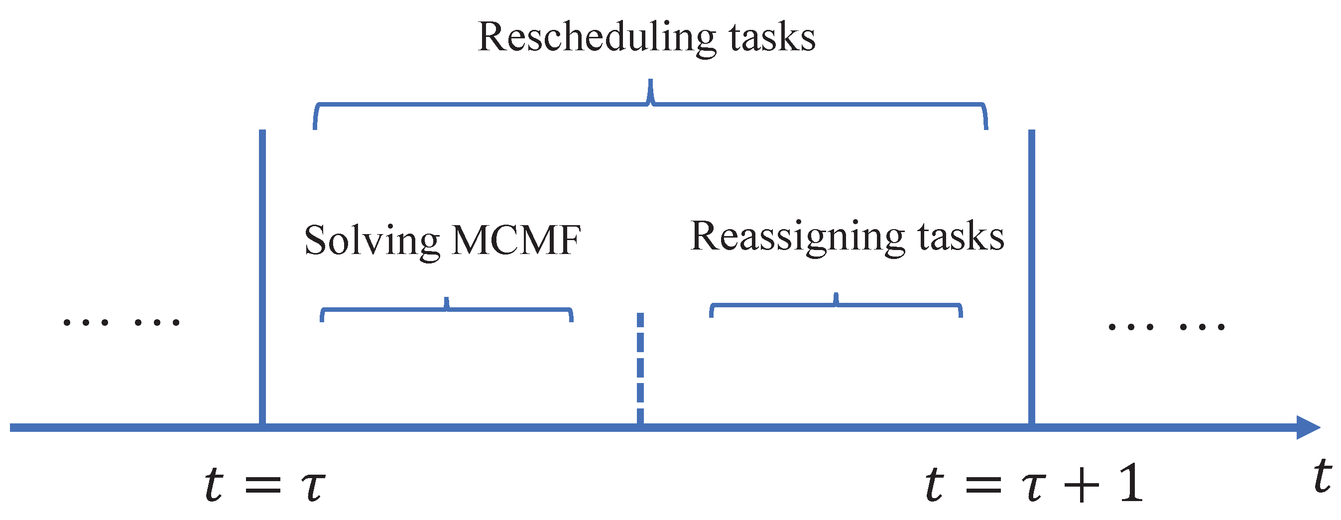
4.2.2. Solving MCMF Incrementally

As stated in Section 4.2, influences of the changes of tasks and hosts on the flow network can be summed up as 7 types: (1) nodes are added; (2) nodes are deleted; (3) supply values b i of some tasks change; (4) arcs are added; (5) arcs are deleted; (6) cost values c i j of some arcs change; and (7) upper capacities u i j of some arcs change.
Generally, algorithms on MCMF problems can be categorized into three types, namely primal, dual, and primal–dual methods [37]. Primal methods, such as cycle cancelling [38] and network simplex [39], try to reduce the overall cost on all arcs by increasing flow along the negative cost loops iteratively. During the process, feasibility of flow f in each iteration is ensured while the optimality is continuously improved until no negative cost loop can be found. On the contrary, dual methods, such as relaxation [40] and successive shortest path [41], optimize the dual problem iteratively based on Lagrangian duality. Optimal flow f can be obtained by keeping the so-called complementary slackness optimality. In this process, reduced cost optimality is maintained while feasibility is improved. Cost scaling [42] is a typical primal-dual method, which has been seen as the most efficient MCMF algorithm. During iterations, both feasibility and optimality are maintained by introducing a new concept called ϵ -complementary slackness optimality.
Since changes on the network usually take place locally, the solving process can be significantly accelerated when MCMF problems are solved incrementally. As stated above, different kinds of algorithms should keep some specific features during an iteration. For primal and primal–dual methods, the feasibility of flow should be ensured in each iteration. On the contrary, complementary slackness is maintained in dual algorithms. As these features are always destroyed after changing the network, these features need to be restored first before reoptimizing the problem. In general, three steps are needed when solving MCMF problems incrementally, namely (1) updating network and the associated data structures; (2) restoring the features of algorithms; and (3) reoptimizing.
Time performance about these algorithms has been studied widely and cost scaling (CS) and network simplex (NS) are recognized as the two most efficient algorithms [37]. To have a more complete analysis, relaxation algorithm together with CS and NS are discussed in detail. In relaxation, flow is increased along an augmenting path to improve the feasibility of f. Destruction on complementary slackness can be easily restored by adjusting flow. In CS, feasibility is maintained and flow f is improved by scaling down ϵ , which can be seen as the error. The smaller ϵ is, the faster CS executes. However, ϵ may change significantly even if only a few arcs change. Experiments in Hapi [43] show that runtime of CS is unpredictable with large variance. In NS, a tree data structure is adopted which can be used to preserve past information. To solve problems incrementally, changes on network need to be reflected on the modification the tree.
Time performance on solving MCMF problems incrementally has been verified in Firmament [18], where only CS2 (a version of CS) and RelaxIV (a version relaxation) were compared. In this paper, CS2, RelaxIV and network simplex are all implemented and compared. In our experiments, the numbers of tasks and hosts are set at 3200 and 1000, respectively. Percentage of changed tasks and hosts increases from 0.001 to 0.2 with a step of 0.001. Experiment results depicted in Figure 4 show that runtime of RelaxIV and NS is proportional to the percentage of changed nodes and arcs. When the percentage is relatively small, significant speed-up can be obtained. Compared to RelaxIV, runtime of NS has a much lower growth rate. As a contrast, although CS has the best time performance when solving MCMF problems from draft, its incremental runtime is un-deterministic with big variance. Surprisingly, its runtime is even longer when only 0.1% of tasks and hosts change. This can be attributed to that some extra operations are needed to adjust corresponding data structures in CS2 before executing reoptimization. Thus, CS2 is not a good choice for the acceleration of solving MCMF problems incrementally. In Pool, NS is adopted to reschedule tasks iteratively.

4.3. Reassigning of Tasks

After obtaining the optimal flow f τ + 1 , task assignment solution F τ + 1 at time τ + 1 is then extracted from it. However, as different solutions can be extracted from the same flow, it will result in a great number of migrations if the assignment solution F τ at time τ is not considered. In this part, we will introduce how to reassign the tasks based on both the optimal flow f τ + 1 and the assignment solution F τ at time τ . The detailed procedures are presented in Algorithm 1.
Algorithm 1: Rescheduling of tasks in Pool
Applsci 12 01646 i001
As tasks are processed sequentially when determining their assignments based on the optimal flow, tasks with larger migration cost should be considered first. In our algorithm, we first calculate the migration cost of each task based on Equation (2), and then sort all tasks in a descending order. Each task has an attribute called isAssigned to indicate whether this task has been assigned to some host at time τ . For a newly added task, this value is set at false. There exists two ways to express the migration cost of task i. On the one hand, a new arc from task i to its corresponding host h can be added to indicate the preference of task i for staying in h. However, it can increase the complexity of flow network markedly. On the other hand, the migration cost of task i can be calculated and taken into consideration when assigning tasks based on optimal flow f. In this case, the structure of flow network needs not to be modified. In Pool, the second strategy is adopted for simplicity.
For task t which has been assigned at time τ , if its corresponding host h is deleted at time τ + 1 , it must be migrated to other hosts and its value of isAssigned is reset at false. Otherwise, we need to justify whether there exists a feasible path between the corresponding task node of t and host node of h in f τ + 1 . If true, it means that assigning t to h confronts to the optimal flow and incurs the least communication cost. In this case, the assignment of t keeps unchanged and the optimal flow f τ + 1 is updated.
However, the non-existence of feasible path between t and h does not mean that task t must be migrated. On the one hand, the reason may be that host h can provide adequate resources while assigning t to some other hosts may incur smaller cost. On the other hand, it can be attributed to that h cannot provide enough resources to process t due to resource competition from other tasks. For the first situation, we need to further verify whether the gain obtained from migrating t can make up the migration cost of t. Communication cost of current assignment and the migration cost for task t can be easily calculated based on Equations (1) and (2), respectively. To be simplified, the minimum communication cost for t in all possible assignments is calculated heuristically to obtain the migration gain (see Lines 14–16 in Algorithm 1). If the gain is less than migration cost, task t is still assigned to host h. Otherwise, value of isAssigned for t is set at false (see Lines 17–22 in Algorithm 1). For the second situation, we just need to set isAssigned at false.
After processing all the tasks, those whose value on isAssigned is false are all stored in list unScheList. At this time, tasks can be assigned in a traditional way without the consideration of task migration based on unScheList and the updated flow f τ + 1 (see Line 35 in Algorithm 1). As this procedure is similar to other flow-based schedulers, it is not described in detail for simplicity.

4.4. Time Complexity of Pool

In each iteration of Pool, two procedures are needed, namely obtaining the optimal flow incrementally and reassigning the tasks based on both the newly obtained optimal flow and the assignments of tasks in the last iteration.
For the first procedure, all the tasks and hosts change in the worst scenario and thus the time complexity equals to solving MCMF problems from draft. Since network simplex is adopted as the MCMF solver, the time complexity is O ( N M 2 C U ) , where N denotes the number of nodes, M the number of arcs, C the maximum value of arc cost, and U the maximum value of arc capacity.
In the second procedure, there exists two extreme situations. If all tasks have been assigned to some hosts in the last iteration (See line 4 in Algorithm 1), the time complexity in this procedure can be denoted as O ( | T | · log ( | T | ) ) + | T | · ( O ( 1 ) + O ( | C | + | E | ) ) = O ( | T | · log ( | T | ) ) . Otherwise, the assignments of tasks should be extracted greedily from the optimal flow, which may incur O ( | T | · | H | ) time complexity. Thus, the time complexity of procedure 2 is max ( O ( | T | · log ( | T | ) ) , O ( | T | · | H | ) ) .
Considering that M > N > | T | > | H | , the overall time complexity of Pool is O ( N M 2 C U ) .

5. Experiments and Analysis

In this section, performance of Pool is analyzed and evaluated. We mainly focus on scheduling tasks efficiently when the status of tasks and hosts changes frequently. Thus, two evaluation indicators are adopted, namely time performance and deployment quality. Time performance is quantified by the time span between the changing of tasks and hosts to the completion of task assignments. Deployment quality is expressed by the overall communication cost of tasks according to Equation (1).
As described in Section 2.2, various algorithms can be adopted to schedule tasks. Since the superiority of flow-based scheduler has been verified in previous studies [17,18,19], we mainly evaluate whether it still works well when the status of tasks and hosts changes frequently. In the design of Pool, optimal flow f τ + 1 is calculated based on incremental MCMF algorithms and task assignments are determined with the consideration of task migration cost. This strategy is called Pool_Inc in the latter parts. For comparison, Pool_nInc is designed, in which f τ + 1 is calculated from the draft and tasks are assigned at time τ + 1 based on only the optimal flow f τ + 1 and current assignments F τ without the consideration of task migration cost. For simplicity, Pool_Inc and Pool_nInc are abbreviated as Inc and nInc, respectively.

5.1. Parameter Settings

In our experiments, Alibaba cluster trace [44] was adopted to generate resource requirements of tasks, as well as resource supplies of hosts. It consists of 13,654 hosts and 116,418 tasks, which are highly heterogeneous and rich in runtime information. In this paper, only number of CPU cores and volume of memory of tasks and hosts were derived from the trace.
To evaluate the performance of Pool in different problem scales, the numbers of hosts were set at 13,654 and 1000, which were also called big and small problem scale, respectively. For each scale, different load levels called Low, Medium, and High were adopted. Details about the number of tasks and hosts are given in Table 1.
However, information about network topology of computation nodes and the communication patters between tasks are not recorded in Alibaba trace. In our experiments, these values were generated randomly. For parameters α , β , γ , and λ , they were all derived from a uniform distribution. Considering that skewed distributions with long tails are much more common in computer workloads, gamma distribution was adopted to generate d i and s i for task i.
As migration cost of each task i T is calculated in Algorithm 1, image size ζ i , task size ł i , task life ρ i and their corresponding coefficients ω 1 , ω 2 , and ω 3 should also be set properly according to Equation (2). Intuitively, tasks with more resource requirements have a large size of ζ i and ł i . In our experiments, ζ i and ł i were set at C 1 · ψ i and C 2 · ψ i , respectively, where ψ i is the required memory size of task i and C 1 and C 2 are two constants sampled from N ( 1 , 5 ) and N ( 0.1 , 1 ) , respectively. Value of ρ i was set for task i during iterations. Values of ω 1 , ω 2 and ω 3 were all set at 0.1. Table 2 shows the detailed parameter settings.
To evaluate the scheduling performance of Pool, status of some tasks and hosts is modified. In our experiments, the percentage of changed tasks and hosts increased from 1% to 100% with step 1%. For a certain number of changed tasks and hosts, three operations were adopted sequentially, namely adding, deleting and changing tasks and hosts. In the third operation, besides the resource requirements of tasks and supplies of hosts were changed, communication patterns of tasks were also modified.

5.2. Experiment Environment

Our experiments were implemented and analysed on Ubuntu 20.04 LTS in a computer with Intel ® i7-7700 8 core CPU (3.60 GHz), and 16 GB RAM. Scheduler Pool was written in C++ and a open source MCMF algorithm library called MCFClass [45] was adopted to obtain the optimal flow. All our experiments were carried out in a simulation environment.

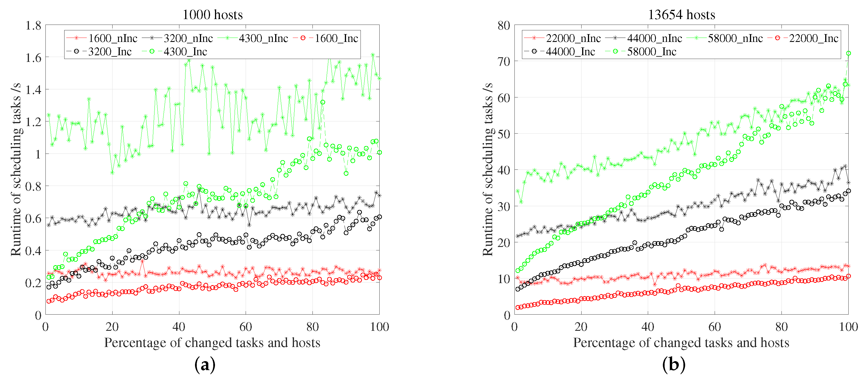
5.3. Time Performance

Considering the frequent changes of the status of tasks and hosts, scheduler should give the approximate optimal assignment decisions as soon as possible. Thus, time performance is an important evaluation metric. In each time step, two procedures are required before obtaining the assignments, namely solving the new MCMF problem and extracting assignments from the generated optimal flow. In this part, runtime consumed in both the procedures is discussed.

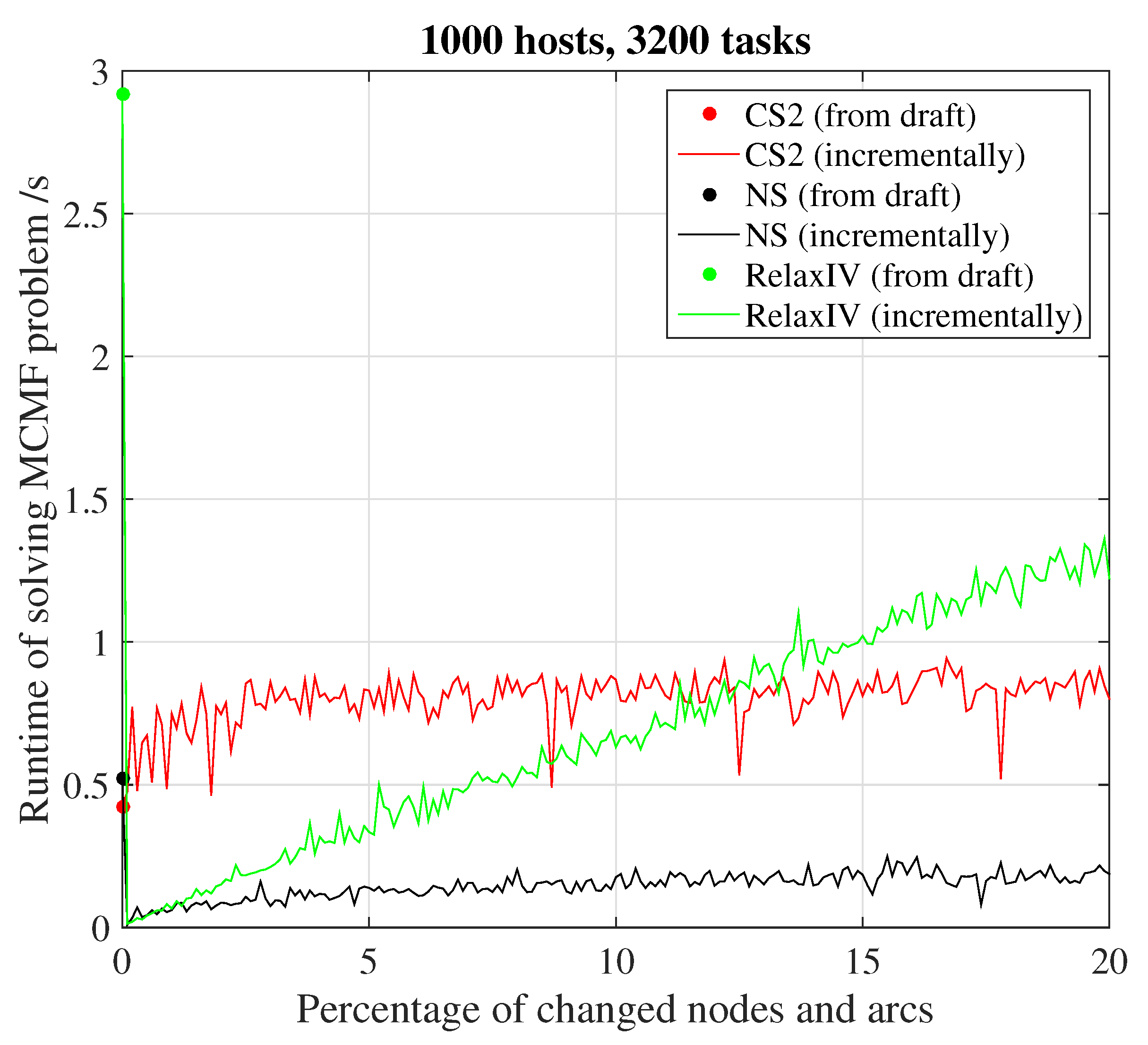
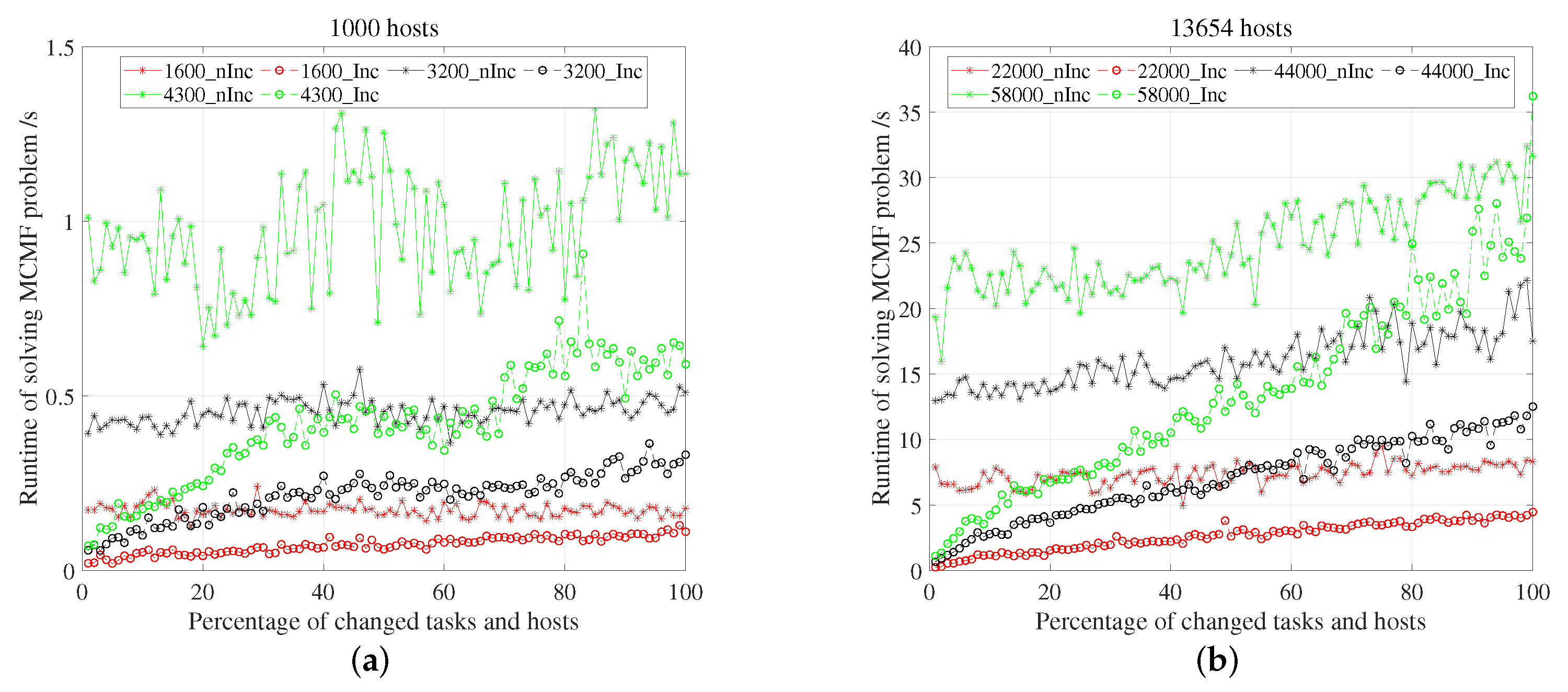
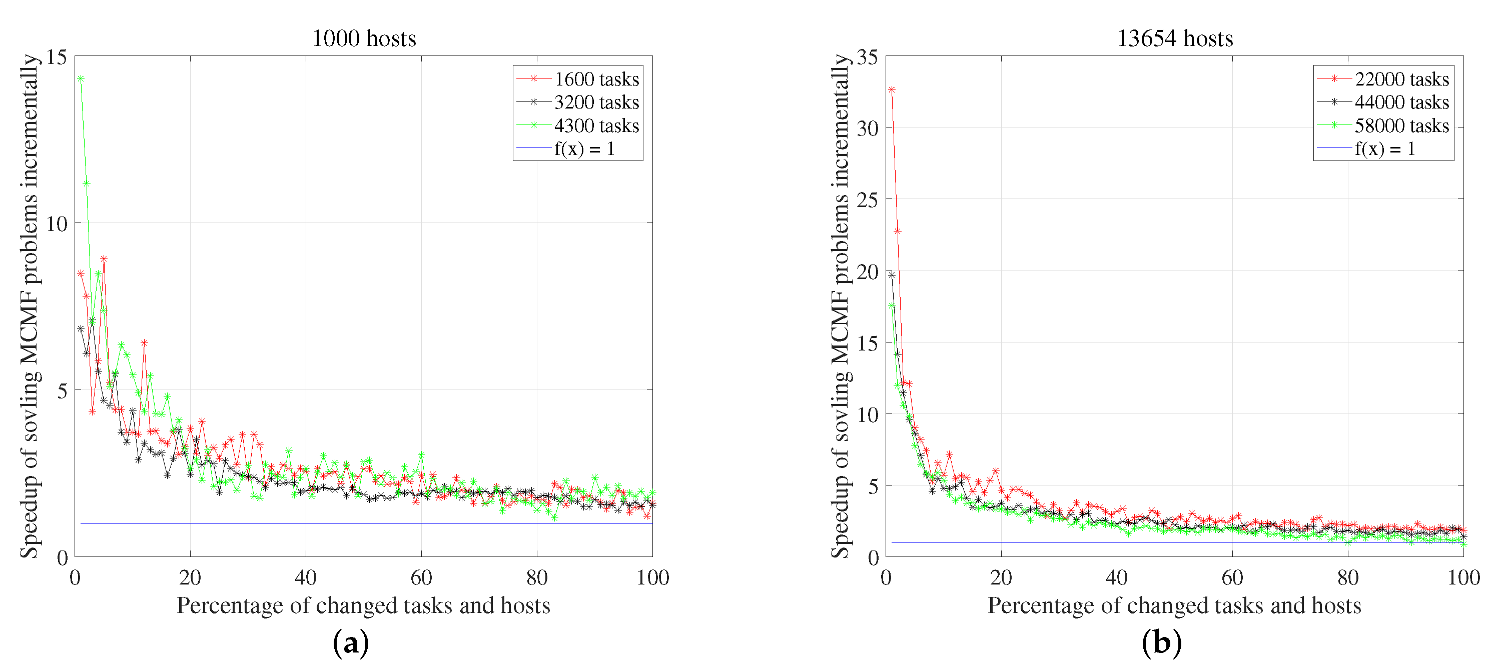
5.3.1. Time in Solving MCMF Problem

Figure 5 depicts the runtime of solving MCMF problems using NS when the numbers of hosts were set at 1000 and 13,654 in different load levels. Figure 5a presents the experiment results when setting the number of hosts at 1000. When solving MCMF problems incrementally, runtime of NS is proportional to the percentage of changed tasks and hosts in all three load levels. The larger the load level, the bigger the growth rate of runtime. This is obvious since more tasks are changed for a certain percentage. On the contrary, runtime of solving MCMF problems from draft increases very slightly, which can be attributed to the polynomial time complexity of NS. At the same time, its variance is very big especially in high load level (4300 tasks). The reason may be that the initial feasible tree adopted in NS algorithm has a great impact on the successive iterative efficiency. Similar conclusions can be obtained when setting the number of hosts at 13,654 in Figure 5b.
To evaluate the improvement on time performance quantitatively, Figure 6 presents the speed-up of solving MCMF problems incrementally compared to solving them from draft. It can be found that the highest speed-up can be obtained when only very few tasks and hosts change. However, it decreases rapidly as the change percentage grows. Still, the value of speed-up is greater than 1 even when all tasks and hosts are modified. In general, there seems to be no significant difference between different load levels in both host settings. As we compare Figure 6a,b horizontally, bigger speed-up can be obtained in a bigger problem scale (13,654 hosts) when the percentage is less than 10%. It means that solving MCMF problems incrementally using NS is well suited for large scale scheduling problems.

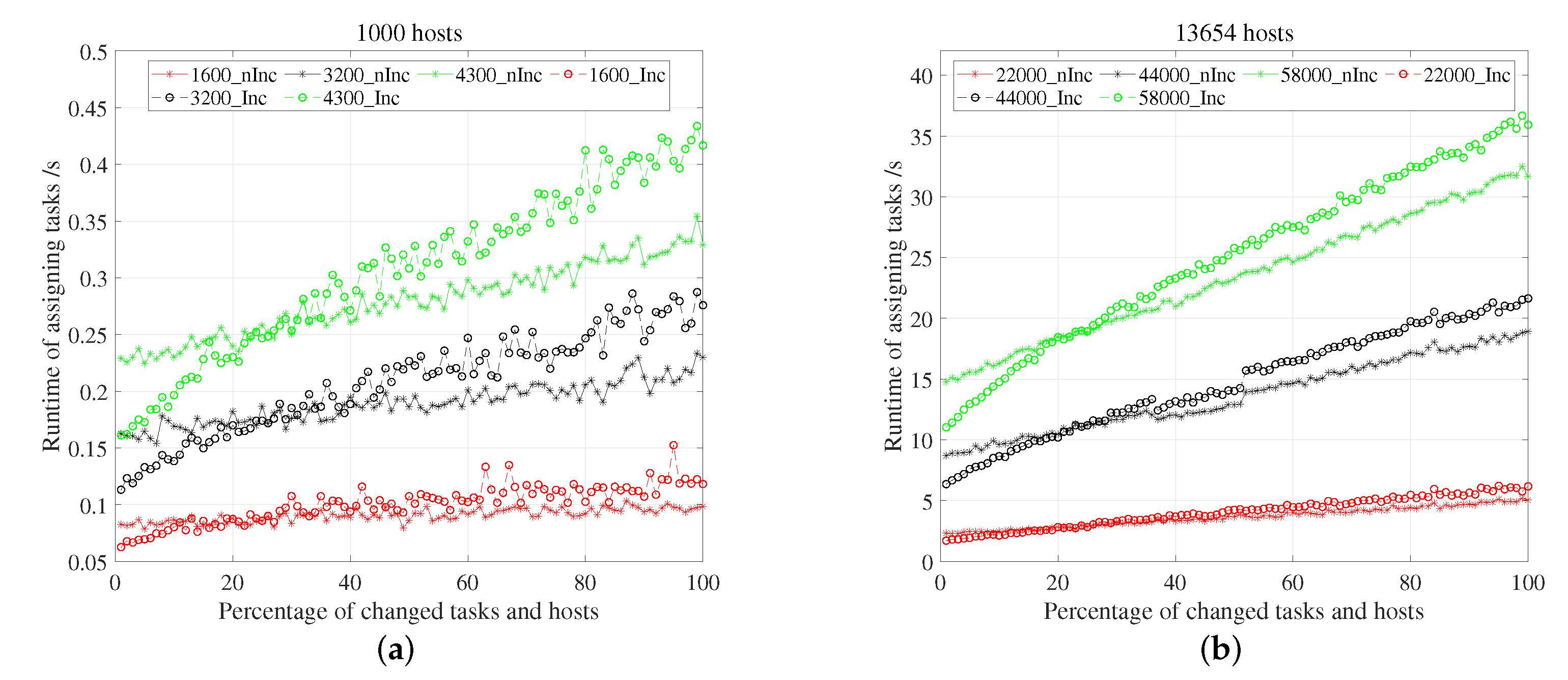
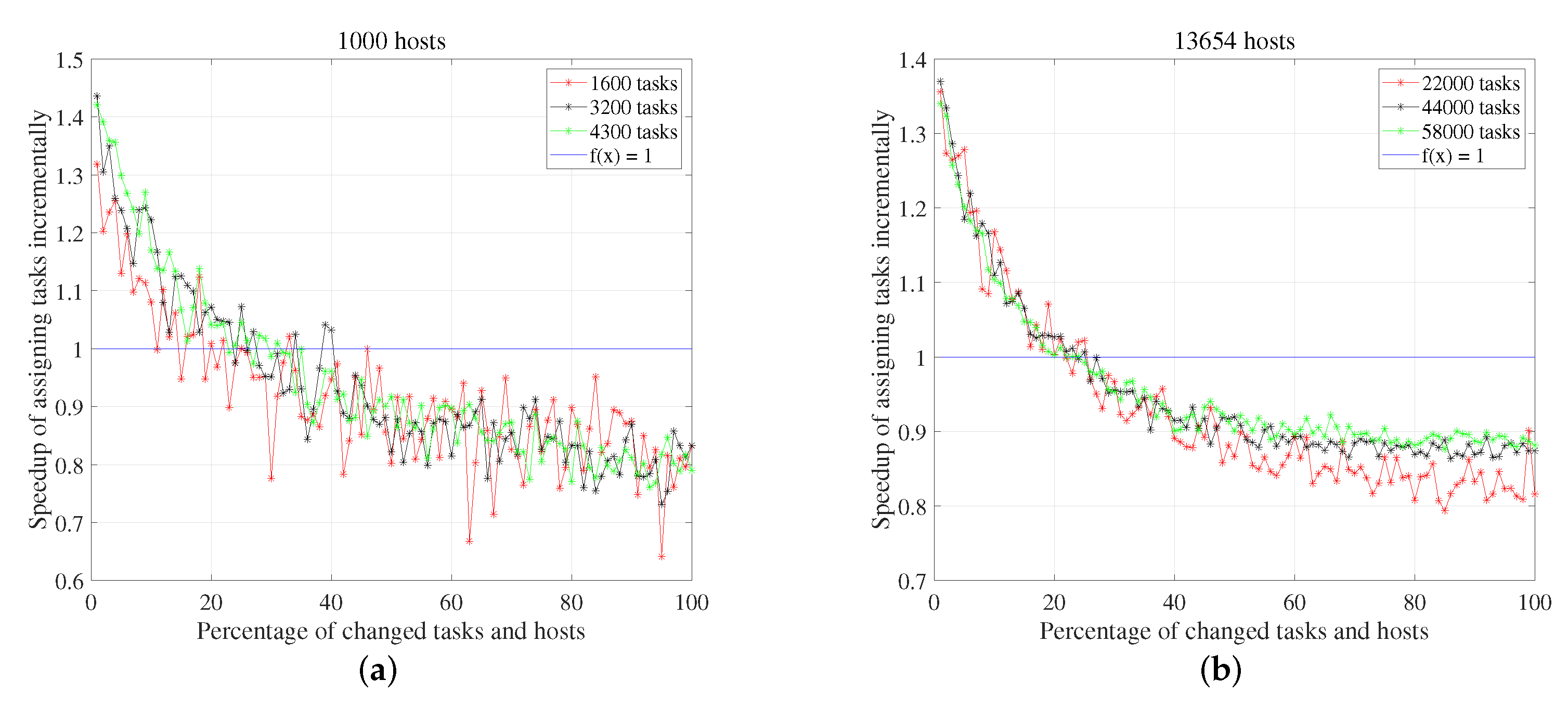
5.3.2. Time in Reassigning Tasks

Runtime of assigning tasks based on the generated optimal flow is given in Figure 7. Figure 7a shows the results when setting the number of hosts at 1000. It can be found that time used to assign tasks in Inc is proportional to the percentage of changed tasks and hosts in all three load levels. The larger the number of tasks, the bigger the slope of growth. On the contrary, runtime of assigning tasks in nInc increases very slightly. In general, Inc is much faster than nInc especially when only a small proportion of tasks and hosts change.
However, situation seems to be much different in Figure 7b. Firstly, we can observe that the difference between Inc and nInc is much smaller. Moreover, after changing certain percentage of tasks and hosts, 18%, for example, when number of tasks is set at 5800, assigning tasks incrementally is even slower. In fact, only constant time complexity is introduced in Inc compared to nInc, except that a sort procedure with time complexity | T | · log ( | T | ) is needed in Inc (See lines 1 in Algorithm 1). This extra overhead can, thus, reduce the overall gains of Inc when the value of | T | is very large.
To evaluate the time performance quantitatively, speed-up of assigning tasks incrementally is given in Figure 8. In can be found that speed-up when setting the number of hosts at 1000 in Figure 8a is greater than 1 for all three levels with less than 20% changed tasks and hosts. However, assigning tasks incrementally consumes more time compared to the traditional method. This means that assigning tasks incrementally is only suitable when only a small proportion of tasks change.
Both of the two procedures of solving MCMF problem and reassigning tasks are required in each time step. Figure 9 presents the overall time performance of Inc and nInc in different problem scales and load levels. We can find that Inc has the better time performance in all cases especially when the changing percentage is relatively small. For example, Inc is almost 5.8 times faster than nInc (0.21 s to 1.22 s) when the numbers of tasks and hosts are set at 4300 and 1000, respectively, and the change percentage is set at 1%.

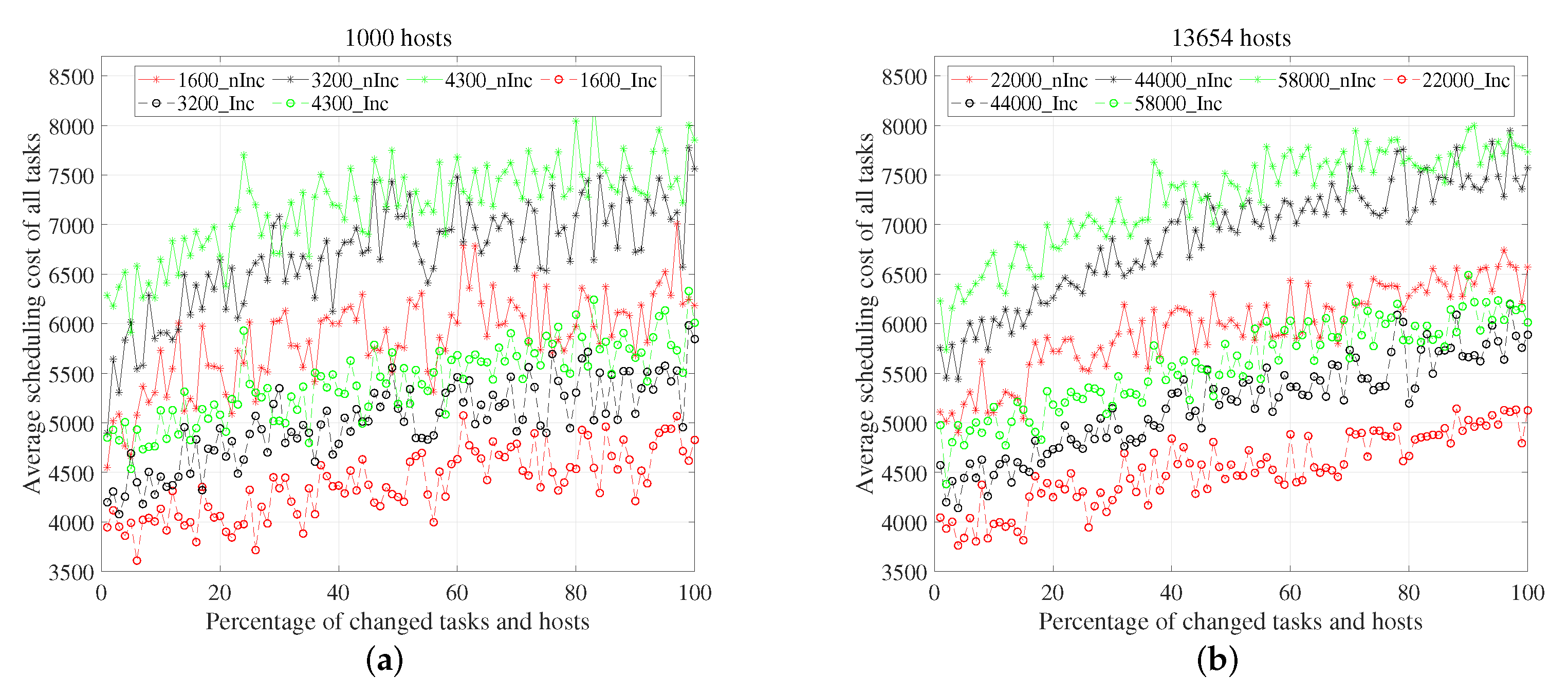
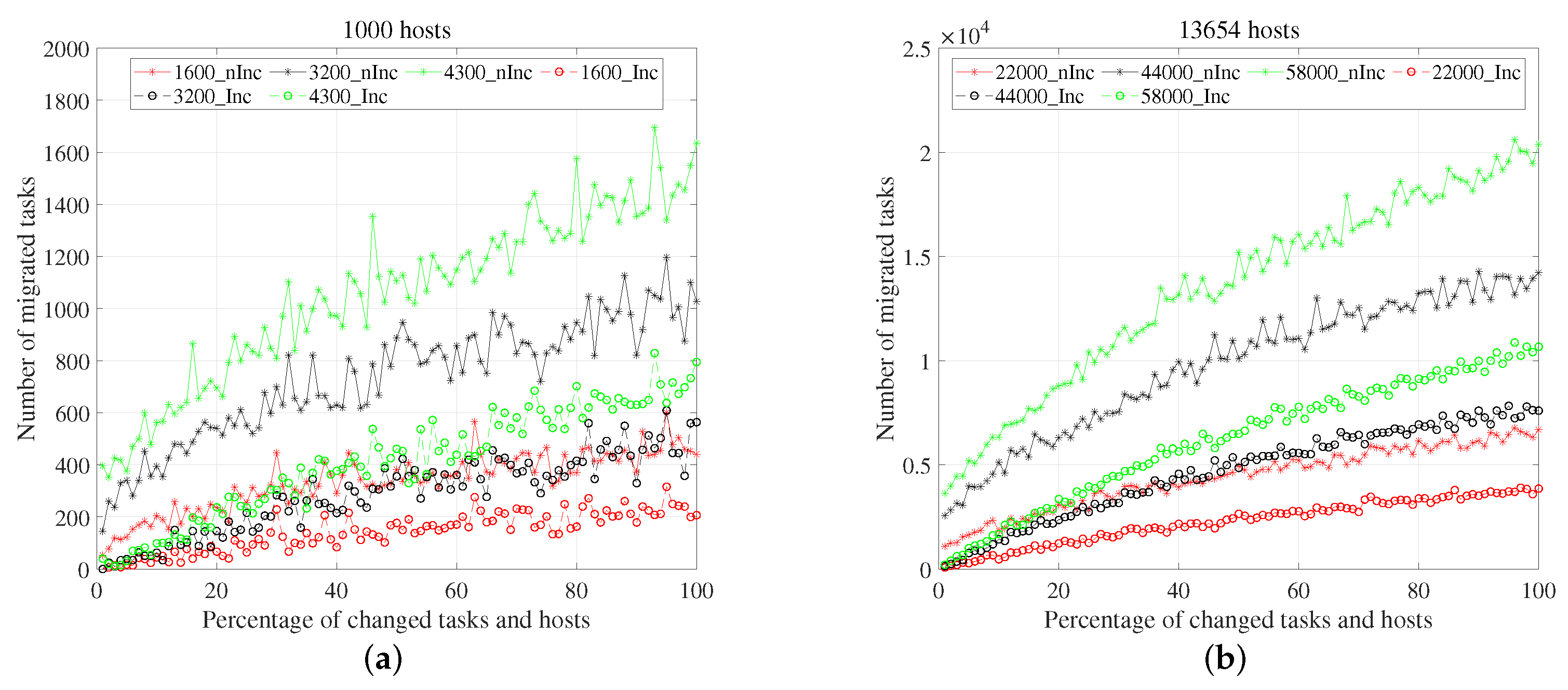
5.4. Deployment Quality

To evaluate the deployment quality of all tasks in each scheduling cycle, average scheduling cost g τ / | T | of all tasks is recorded. As depicted in Equation (3), scheduling cost of a task can be divided as communication and migration cost, which can be calculated according to Equations (1) and (2), respectively.
The average scheduling cost of all tasks is given in Figure 10. For all three load levels and two settings of hosts, the value of scheduling cost increases with a big variance as the percentage grows. This can be attributed to the randomness when changing tasks and hosts. For example, adding and deleting of some tasks with large amount of resource requirements and high communication strength have a huge impact on the overall communication cost. However, for a certain load level and changing percentage, we can observe that average scheduling cost of Inc is slightly bigger than that of nInc. The reason for this phenomenon is that migration cost of tasks is not considered in nInc. As shown in Equation (3), we should minimize the sum of communication cost and migration cost of all tasks.
To study the impact of migration cost on the overall deployment quality, the number of migrated tasks are given in Figure 11. We can observe from both subgraphs that more tasks are migrated with the increase in changing percentage. For all load levels, the number of migrated tasks in Inc are much smaller than that in nInc, especially when status of a big proportion of tasks and hosts are modified. As some tasks are not assigned based on the optimal flow (See lines 15–25 in Algorithm 1), results in Figure 11 show why Inc has a better performance on the deployment quality of all tasks.

6. Conclusions and Future Work

In this paper, we mainly focus on the efficient scheduling of simulation tasks in a collaborative cloud and edge environment, especially when the status of tasks and hosts changes frequently. We present a new scheduler called Pool and the main goal of Pool is to minimize the overall communication cost and migration cost of all tasks in a reasonable time span.
Firstly, such a combinational optimization problem is formulated as a MCMF problem by relaxing some constraints and network simplex is adopted as the solver. When the status of tasks and hosts changes, the corresponding MCMF problem is also modified. To improve the time performance of Pool, MCMF problem is solved incrementally by utilizing the past information. Moreover, tasks are rescheduled heuristically with the consideration of both past assignments and task migration cost. Extensive simulation experiments are conducted based on Alibaba cluster trace and the results show that Pool can efficiently accelerate the solving process of MCMF problems especially when the proportion of changed tasks and hosts is relatively small. At the same time, the number of migrated tasks can be minimized without increasing the overall communication cost. In the future, we plan to implement Pool in a real simulation scenario to verify its effectiveness.

Author Contributions

Conceptualization, M.Z.; Formal analysis, M.Z. and Y.P.; Investigation, P.J. and Y.P.; Methodology, M.Z.; Project administration, Q.Y.; Resources, Q.Y.; Supervision, Q.Y. All authors have read and agreed to the published version of the manuscript.

Funding

This research was supported in part by National Natural Science Foundation of China (Grant NO. 62103425 and 62103428) and Natural Science Foundation of Hunan Province (Grant No. 2021JJ40697).

Institutional Review Board Statement

Not applicable.

Informed Consent Statement

Not applicable.

Data Availability Statement

Not applicable.

Conflicts of Interest

The authors declare no conflict of interest.

References

  1. Peter Mell, T.G. The NIST Definition of Cloud Computing. Available online: https://csrc.nist.gov/publications/detail/sp/800-145/final (accessed on 24 November 2021).
  2. DoD. Defense Modeling and Simulation Reference Architecture, Version 1.0. 2020. Available online: https://www.msco.mil/MSReferences/PolicyGuidance.aspx (accessed on 24 November 2021).
  3. Fujimoto, R.; Bock, C.; Chen, W.; Page, E.; Panchal, J.H. Research Challenges in Modeling and Simulation for Engineering Complex Systems; Springer: Berlin/Heidelberg, Germany, 2017. [Google Scholar] [CrossRef]
  4. Taylor, S.J. Distributed simulation: State-of-the-art and potential for operational research. Eur. J. Oper. Res. 2019, 273, 1–19. [Google Scholar] [CrossRef] [Green Version]
  5. Fujimoto, R.M.; Malik, A.W.; Park, A. Parallel and distributed simulation in the cloud. SCS M&S Mag. 2010, 3, 1–10. [Google Scholar]
  6. Shi, W.; Cao, J.; Zhang, Q.; Li, Y.; Xu, L. Edge Computing: Vision and Challenges. IEEE Internet Things J. 2016, 3, 637–646. [Google Scholar] [CrossRef]
  7. Miao, Z.; Yong, P.; Mei, Y.; Quanjun, Y.; Xu, X. A discrete PSO-based static load balancing algorithm for distributed simulations in a cloud environment. Future Gener. Comput. Syst. 2021, 115, 497–516. [Google Scholar] [CrossRef]
  8. Verma, A.; Pedrosa, L.; Korupolu, M.; Oppenheimer, D.; Tune, E.; Wilkes, J. Large-Scale Cluster Management at Google with Borg. In Proceedings of the Tenth European Conference on Computer Systems, EuroSys ’15, Bordeaux, France, 21–24 April 2015; Association for Computing Machinery: New York, NY, USA, 2015. [Google Scholar] [CrossRef] [Green Version]
  9. Zhao, L.; Yang, Y.; Zhang, K.; Zhou, X.; Qiu, T.; Li, K.; Bao, Y. Rhythm: Component-Distinguishable Workload Deployment in Datacenters. In Proceedings of the Fifteenth European Conference on Computer Systems, EuroSys ’20, Heraklion, Greece, 27–30 April 2020; Association for Computing Machinery: New York, NY, USA, 2020. [Google Scholar] [CrossRef]
  10. Delgado, P.; Didona, D.; Dinu, F.; Zwaenepoel, W. Job-Aware Scheduling in Eagle: Divide and Stick to Your Probes. In Proceedings of the Seventh ACM Symposium on Cloud Computing, SoCC ’16, Santa Clara, CA, USA, 5–7 October 2016; Association for Computing Machinery: New York, NY, USA, 2016; pp. 497–509. [Google Scholar] [CrossRef] [Green Version]
  11. Fu, Z.; Tang, Z.; Yang, L.; Liu, C. An Optimal Locality-Aware Task Scheduling Algorithm Based on Bipartite Graph Modelling for Spark Applications. IEEE Trans. Parallel Distrib. Syst. 2020, 3, 2406–2420. [Google Scholar] [CrossRef]
  12. Hu, Z.; Li, B.; Chen, C.; Ke, X. FlowTime: Dynamic Scheduling of Deadline-Aware Workflows and Ad-Hoc Jobs. In Proceedings of the IEEE International Conference on Distributed Computing Systems, Vienna, Austria, 2–6 July 2018. [Google Scholar]
  13. Liu, C.; Li, K.; Li, K. A Game Approach to Multi-Servers Load Balancing with Load-Dependent Server Availability Consideration. IEEE Trans. Cloud Comput. 2021, 9, 1–13. [Google Scholar] [CrossRef]
  14. Talbi, E.G. Metaheuristics: From Design to Implementation; John Wiley & Sons: Hoboken, NJ, USA, 2009; Volume 74. [Google Scholar] [CrossRef]
  15. Ghodsi, A.; Zaharia, M.; Hindman, B.; Konwinski, A.; Shenker, S.; Stoica, I. Dominant Resource Fairness: Fair Allocation of Multiple Resource Types. In Proceedings of the 8th USENIX Conference on Networked Systems Design and Implementation, NSDI’11, Boston, MA, USA, 30 March–1 April 2011; USENIX Association: San Jose, CA, USA, 2011; pp. 323–336. [Google Scholar]
  16. Govil, A.K. Priority Assignment in waiting line problem. Trab. Estad. Investig. Oper. 1971, 22, 97–103. [Google Scholar] [CrossRef]
  17. Isard, M.; Prabhakaran, V.; Currey, J.; Wieder, U.; Talwar, K.; Goldberg, A. Quincy: Fair Scheduling for Distributed Computing Clusters. In Proceedings of the ACM SIGOPS 22nd Symposium on Operating Systems Principles, SOSP ’09, Big Sky, MT, USA, 11–14 October 2009; Association for Computing Machinery: New York, NY, USA, 2009; pp. 261–276. [Google Scholar] [CrossRef]
  18. Gog, I.; Schwarzkopf, M.; Gleave, A.; Watson, R.N.M.; Hand, S. Firmament: Fast, Centralized Cluster Scheduling at Scale. In Proceedings of the 12th USENIX Conference on Operating Systems Design and Implementation, OSDI’16, Savannah, GA, USA, 2–4 November 2016; USENIX Association: San Jose, CA, USA, 2016; pp. 99–115. [Google Scholar]
  19. Wu, H.; Zhang, W.; Xu, Y.; Xiang, H.; Zhang, Z. Aladdin: Optimized Maximum Flow Management for Shared Production Clusters. In Proceedings of the 2019 IEEE International Parallel and Distributed Processing Symposium (IPDPS), Rio de Janeiro, Brazil, 20–24 May 2019. [Google Scholar]
  20. Jin, T.; Cai, Z.; Li, B.; Zheng, C.; Jiang, G.; Cheng, J. Improving Resource Utilization by Timely Fine-Grained Scheduling. In Proceedings of the Fifteenth European Conference on Computer Systems, EuroSys ’20, Heraklion, Greece, 27–30 April 2020; Association for Computing Machinery: New York, NY, USA, 2020. [Google Scholar] [CrossRef]
  21. Delimitrou, C.; Sanchez, D.; Kozyrakis, C. Tarcil: Reconciling Scheduling Speed and Quality in Large Shared Clusters. In Proceedings of the Sixth ACM Symposium on Cloud Computing, SoCC ’15, Kohala Coast, HI, USA, 27–29 August 2015; Association for Computing Machinery: New York, NY, USA, 2015; pp. 97–110. [Google Scholar] [CrossRef] [Green Version]
  22. Park, J.W.; Tumanov, A.; Jiang, A.; Kozuch, M.A.; Ganger, G.R. 3Sigma: Distribution-based cluster scheduling for runtime uncertainty. In Proceedings of the Thirteenth EuroSys Conference, Porto, Portugal, 23–26 April 2018. [Google Scholar]
  23. Boutin, E.; Ekanayake, J.; Lin, W.; Shi, B.; Zhou, J.; Qian, Z.; Wu, M.; Zhou, L. Apollo: Scalable and Coordinated Scheduling for Cloud-Scale Computing. In Proceedings of the 11th USENIX Conference on Operating Systems Design and Implementation, Broomfield, CO, USA, 6–8 October 2014; OSDI’14. USENIX Association: San Jose, CA, USA, 2014; pp. 285–300. [Google Scholar]
  24. Forestiero, A.; Mastroianni, C.; Meo, M.; Papuzzo, G.; Sheikhalishahi, M. Hierarchical approach for green workload management in distributed data centers. In Proceedings of the European Conference on Parallel Processing, Porto, Portugal, 25–29 August 2014; pp. 323–334. [Google Scholar]
  25. Curino, C.; Krishnan, S.; Karanasos, K.; Rao, S.; Fumarola, G.M.; Huang, B.; Chaliparambil, K.; Suresh, A.; Chen, Y.; Heddaya, S.; et al. Hydra: A Federated Resource Manager for Data-Center Scale Analytics. In Proceedings of the 16th USENIX Conference on Networked Systems Design and Implementation, NSDI’19, Boston, MA, USA, 26–28 February 2019; USENIX Association: San Jose, CA, USA, 2019; pp. 177–191. [Google Scholar]
  26. Delgado, P.; Dinu, F.; Kermarrec, A.M.; Zwaenepoel, W. Hawk: Hybrid Datacenter Scheduling. In Proceedings of the Usenix Conference on Usenix Technical Conference, Santa Clara, CA, USA, 8–10 July 2015. [Google Scholar]
  27. Saleh, H.; Nashaat, H.; Saber, W.; Harb, H.M. IPSO task scheduling algorithm for large scale data in cloud computing environment. IEEE Access 2018, 7, 5412–5420. [Google Scholar] [CrossRef]
  28. Passino, K.M. Biomimicry of bacterial foraging for distributed optimization and control. IEEE Control. Syst. Mag. 2002, 22, 52–67. [Google Scholar] [CrossRef]
  29. Tang, L.; Li, Z.; Ren, P.; Pan, J.; Lu, Z.; Su, J.; Meng, Z. Online and offline based load balance algorithm in cloud computing. Knowl. Based Syst. 2017, 138, 91–104. [Google Scholar] [CrossRef]
  30. Pourghaffari, A.; Barari, M.; Sedighian Kashi, S. An efficient method for allocating resources in a cloud computing environment with a load balancing approach. Concurr. Comput. Pract. Exp. 2019, 31, e5285. [Google Scholar] [CrossRef]
  31. Kabir, M.S.; Kabir, K.M.; Islam, R. Process of load balancing in cloud computing using genetic algorithm. Electr. Comput. Eng. Int. J. 2015, 4. [Google Scholar] [CrossRef] [Green Version]
  32. Gupta, A.; Garg, R. Load balancing based task scheduling with ACO in cloud computing. In Proceedings of the 2017 International Conference on Computer and Applications (ICCA), Doha, United Arab Emirates, 6–7 September 2017; pp. 174–179. [Google Scholar]
  33. Cplex-Optimizer. Available online: https://www.ibm.com/analytics/cplex-optimizer (accessed on 24 November 2021).
  34. Garefalakis, P.; Karanasos, K.; Pietzuch, P.; Suresh, A.; Rao, S. Medea: Scheduling of long running applications in shared production clusters. In Proceedings of the Thirteenth EuroSys Conference, Porto, Portugal, 23–26 April 2018. [Google Scholar]
  35. Manco, F.; Lupu, C.; Schmidt, F.; Mendes, J.; Kuenzer, S.; Sati, S.; Yasukata, K.; Raiciu, C.; Huici, F. My VM is Lighter (and Safer) than Your Container. In Proceedings of the 26th Symposium on Operating Systems Principles, SOSP ’17, Shanghai, China, 28–31 October 2017; Association for Computing Machinery: New York, NY, USA, 2017; pp. 218–233. [Google Scholar] [CrossRef] [Green Version]
  36. The First DIMACS International Algorithm Implementation Challenge: Problem Definitions and Specifications; Technical Report; Centre for Discrete Mathematics and Theoretical Computer Science (DIMACS): New Brunswick, NJ, USA, 1991.
  37. Király, Z.; Kovács, P. Efficient implementations of minimum-cost flow algorithms. Acta Univ. Sapientiae Inform. 2012, 4, 67–118. [Google Scholar]
  38. Klein, M. A Primal Method for Minimal Cost Flows with Applications to the Assignment and Transportation Problems. Manag. Sci. 1967, 14, 205–220. [Google Scholar] [CrossRef] [Green Version]
  39. Orlin, J.B. A polynomial time primal network simplex algorithm for minimum cost flows. Math. Program. 1997, 78, 109–129. [Google Scholar] [CrossRef]
  40. Bertsekas, D.; Tseng, P. Relaxation Method for Minimum Cost Ordinary Network Flow Problems. Oper. Res. 1988, 36, 93–115. [Google Scholar] [CrossRef] [Green Version]
  41. Ahuja, R.K.; Magnanti, T.L.; Orlin, J.B. Network flows—Theory, algorithms and applications. J. Oper. Res. Soc. 1993, 45, 791–796. [Google Scholar]
  42. Goldberg, A.V. An Efficient Implementation of a Scaling Minimum-Cost Flow Algorithm. J. Algorithms 1997, 22, 1–29. [Google Scholar] [CrossRef] [Green Version]
  43. Gleave, A. Fast and Scalable Cluster Scheduling Using Flow Networks; Computer Science Tripos Part II Dissertation; Computer Laboratory St John’s College, University of Cambridge: Cambridge, UK, 2015. [Google Scholar]
  44. Alibaba Cluster. Available online: https://github.com/alibaba/clusterdata (accessed on 24 November 2021).
  45. Antonio Frangioni, C.G.; Bertsekas, D.P. MCFClass Project. Available online: https://frangio68.github.io/Min-Cost-Flow-Class/ (accessed on 24 November 2021).
Figure 1. Work flow in Pool.
Applsci 12 01646 g001
Figure 2. Network structure in Pool.
Applsci 12 01646 g002
Figure 3. Influences of changing tasks on the network structure.
Applsci 12 01646 g003
Figure 4. Runtime of different MCMF algorithms.
Applsci 12 01646 g004
Figure 5. Runtime of NS when solving MCMF problems incrementally in different load levels. In the legends of figure, number denotes how many tasks are considered, and nInc or Inc indicates the corresponding MCMF problem is solved from draft or incrementally, respectively. (a) 1000 hosts. (b) 13,654 hosts.
Applsci 12 01646 g005
Figure 6. Speed-up of solving MCMF problems incrementally compared to solving them from draft. (a) 1000 hosts. (b) 13,654 hosts.
Applsci 12 01646 g006
Figure 7. Runtime of assigning tasks based on the generated optimal flow. (a) 1000 hosts. (b) 13,654 hosts.
Applsci 12 01646 g007
Figure 8. Speed-up of assigning tasks incrementally. (a) 1000 hosts. (b) 13,654 hosts.
Applsci 12 01646 g008
Figure 9. Runtime of scheduling tasks. (a) 1000 hosts. (b) 13,654 hosts.
Applsci 12 01646 g009
Figure 10. Average scheduling cost of all tasks. (a) 1000 hosts. (b) 13,654 hosts.
Applsci 12 01646 g010
Figure 11. Number of migrated tasks. (a) 1000 hosts. (b) 13,654 hosts.
Applsci 12 01646 g011
Table 1. Workload settings for the experiments.
No. of HostsNo. of Tasks
Low LoadMedium LoadHigh Load
1000160032004300
13,65422,00044,00058,000
Table 2. Parameter settings for the experiments.
SymbolValueDescription
| C | 20Number of data centers
| E | 100Number of edge nodes
| R | 100Number of regions
d i τ Γ ( 3 , 17 ) MBVolume of interactive data between user and task i
s i τ Γ ( 3 , 17 ) MBTotal volume of interactive data for task i
ζ i ψ i · N ( 1 , 5 ) Image size for task i
ł i ψ i · N ( 0.1 , 1 ) Task size for task i
α r c (50,200) ms/MBUnit transferring cost between region r and datacentre c
β r e (10,30) ms/MBUnit transferring cost between region r and edge e
γ e c (50,200) ms/MBUnit transferring cost between edge e and datacentre c
λ k l (50,200) ms/MBUnit transferring cost between datacentre k and l
Publisher’s Note: MDPI stays neutral with regard to jurisdictional claims in published maps and institutional affiliations.

