Deep Q-Network Approach for Train Timetable Rescheduling Based on Alternative Graph

Abstract

The disturbance of local areas with complex railway networks and high traffic density not only impedes the efficient use of rail networks in those areas, but also propagates delays to the entire railway network. This has motivated research on train rescheduling problems in high-density local areas to minimize train delays by modifying their planned arrival and departure times. In this paper, we present a train rescheduling method based on Q-learning in reinforcement learning. More specifically, we used deep neural networks to approximate the action-value function, and the underlying Markov decision process (MDP) is based on the alternative graph formulation for the train rescheduling problem. In the proposed MDP formulation, the status of the alternative graph corresponding to the current schedule is defined as the state, and the alternative arc corresponds to the action the agent can take. The MDP is approximately solved via deep Q-learning in which deep neural networks are used to approximate the action-value function in Q-learning. Although the size of the alternative graph depends on the number of trains, our MDP formulation is independent of the number of trains, which makes the proposed method more scalable. The evaluation of the method was performed on a simple railway network and a real-world example in Seoul, South Korea, with randomly generated initial train schedules and train delays. The experimental result showed that the proposed method is comparable to the mixed-integer-linear-programming (MILP)-based exact approach with respect to the quality of the solution.

1. Introduction

When a train delay occurs on a complex railway network with high traffic density, this delay can be propagated to the entire railway network. This spread hinders the efficient use of railway networks and causes a decrease in the service quality of passenger or freight transportation.

This study addresses train timetable rescheduling (TTR) (also called train dispatching or conflict detection and resolution) in a high-density local area to minimize the knock-on train delays in cases of disturbances that make it impossible to comply with the pre-planned train schedule. Here, “disturbance” means a relatively small perturbation that can be dealt with only by modifying the timetable, different from “disruption”, which requires a change in the duty of a rolling-stock or crew. The TTR problem has been intensively studied in various works, and an overview of the various models and algorithms for this purpose can be found in [1].

Except for some macroscopic models [2,3], most of the models for TTR are microscopic models [4,5,6,7,8,9,10], which allow more-accurate runtime calculations by simulating train movement in detail, down to the microscopic level. One of the mathematical tools to describe these microscopic movements of trains is the alternative graph, used in most microscopic models, which graphically expresses the order in which the trains occupy a common block, as well as a sequence of blocks that each train traverses. For example, the decision variables of several integer programming models are the entry/exit times at the blocks in the alternative graph [7,8,9], and several heuristics are explicitly based on the alternative graph model [4,5,10].

TTR can be modeled as an integer programming model from which we can obtain the optimal solution using branch-and-bound methods or their variants (e.g., branch-and-cut, branch-and-price-and-cut, etc.). However, TTR arises in real-time problem settings in which the solution needs to be provided very quickly. This requirement is hardly satisfied with the existing exact approaches. To address this limitation, several heuristics have been proposed, but there is still a demand for research to find a compromise in the trade-off between the quality of the solution and the computation time.

Recently, reinforcement learning has been applied to TTR, in which, instead of finding the arrival and departure times of trains as a solution, a policy or rule is learned such that any legitimate instances can be solved with this policy [11,12,13,14,15,16]. Since the learned policy does not need to search large solution spaces, new train schedules are quickly provided, and previous studies showed that, if properly learned, the quality of the solution provided by reinforcement learning is compatible with the optimal one. Adopting reinforcement learning for TTR has been further extended to the setting of multi-agent reinforcement learning [17,18], in which each train is regarded as an independent agent. In this paper, however, we are interested in the setting of single-agent reinforcement learning.

Šemrov et al. [11] proposed a reinforcement learning approach for TTR in which the state, the input of the policy, is defined as the train location over blocks; the action, the output of the policy, represents the go or stop signal installed at each block; the transitions of the state with respect to the selected action are made with a “customized” simulation tool. The proposed method was tested on a simple railway network with no junctions.

In TTR, the schedule of a train is likely to affect those of other trains. Some previous studies [12,14] considered this aspect by defining the state as the occupancy information of several or all blocks. More specifically, the occupancy information of each block is represented as the congestion level of that block computed using the number of trains running on the block. However, this representation of states lacks the entry/exit timing and order of trains at each block, which are important in deciding a good schedule, especially for a railway network with junctions.

The current literature defines a policy as the decision rule of a local dispatcher who is responsible for determining the schedule of a single or multiple trains over a small area in a railway network. To directly consider the possible propagation of a delay over the entire network, the arrival and departure times of all trains can be considered as a state [13]. However, this approach was only tested on a simple railway network, where one-way trains run in a single line.

Overall, all of the above studies have limitations in applying their reinforcement learning to more-realistic railway networks with multi-aspect signals or junctions where two trains may converge or diverge. To overcome these limitations, we propose a reinforcement learning approach in which the alternative graph is used for defining the states and actions. More specifically, we define the state using the current topology of the alternative graph and the action for the selection of an alternative arc on the alternative graph. This enables our model to reflect train movement and conflicts between trains at the microscopic level. Furthermore, the proposed method is also applicable to local areas with high traffic density and complex infrastructures such as signaling systems and junctions.

The remainder of this paper is organized as follows. This section continues with a formal statement of the TTR problem based on the alternative graph and the necessary notations. The proposed framework of reinforcement learning is described in Section 2. In Section 3, we demonstrate the numerical results, which verify the performance of the proposed method. Finally, in Section 4, we give some concluding remarks.

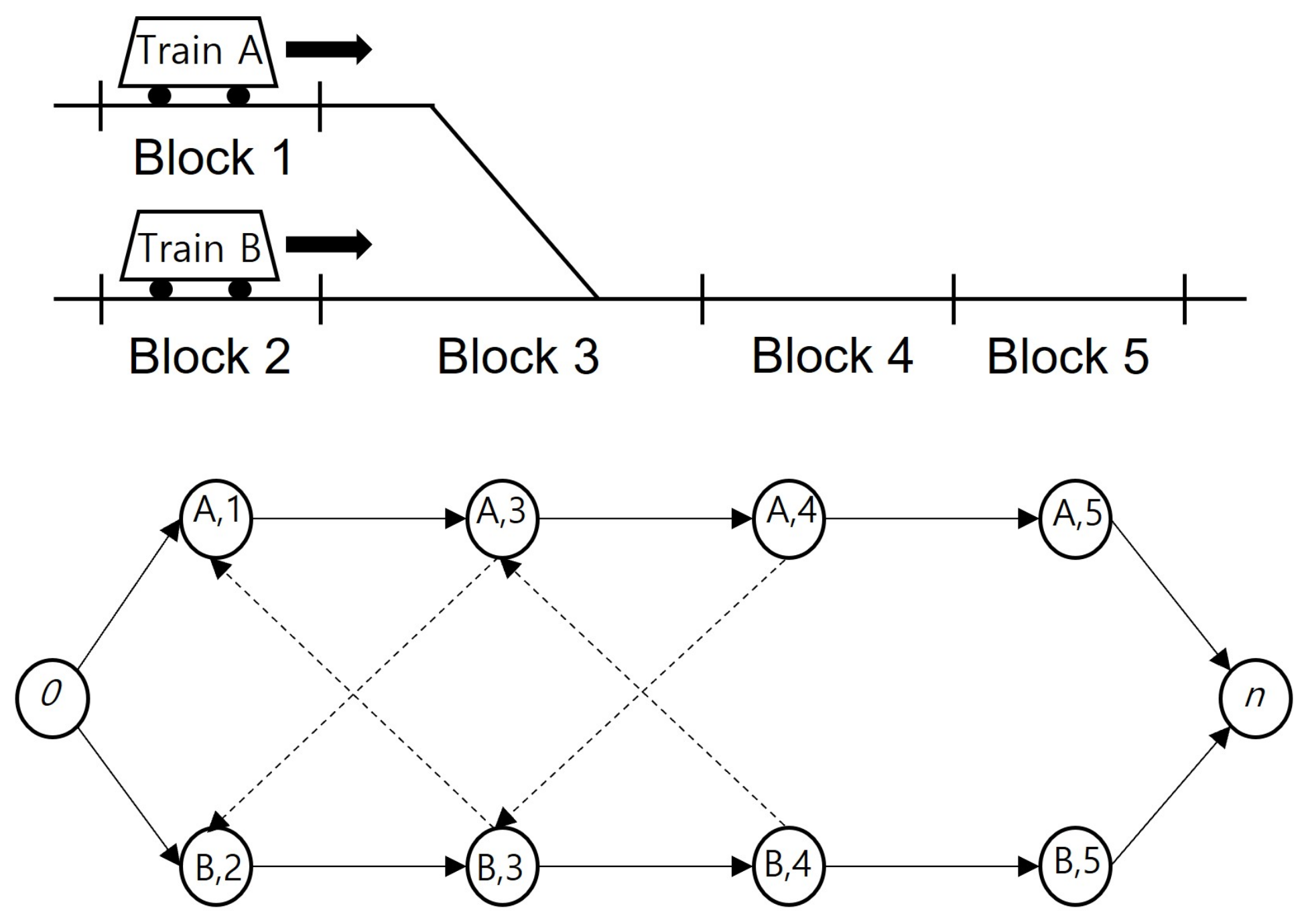
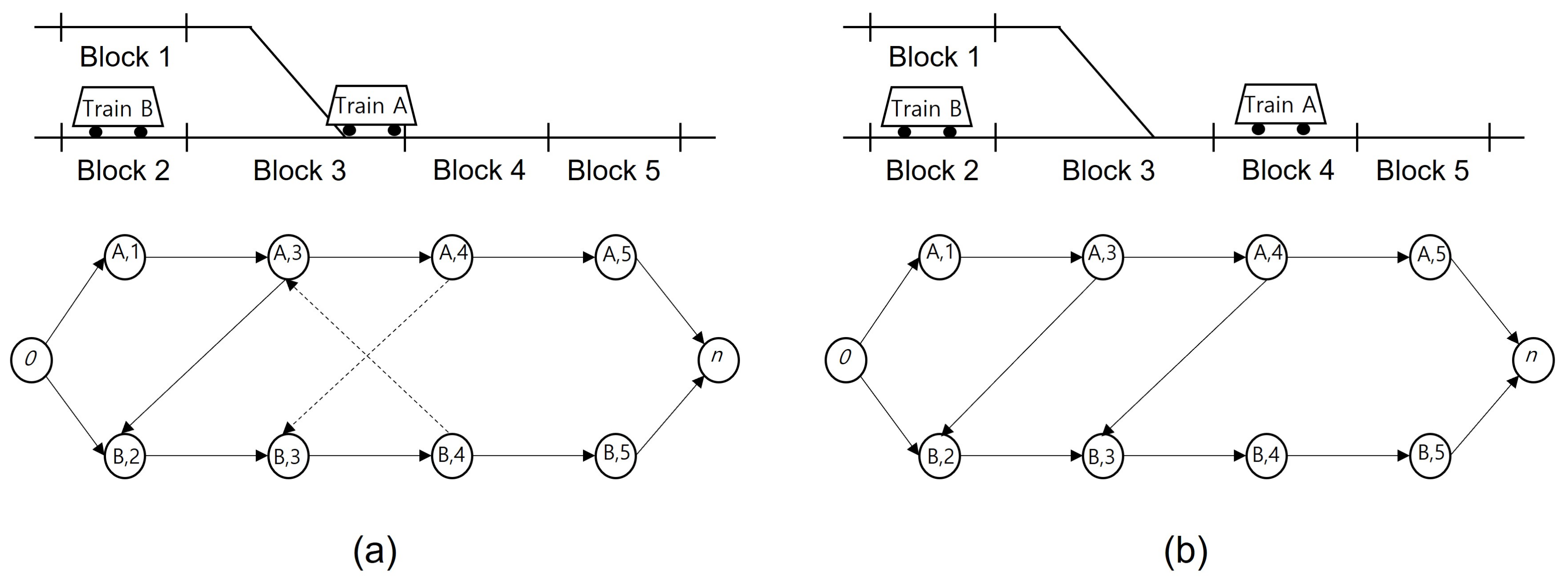
1.1. Preliminary TTR Based on Alternative Graph

We considered a TTR problem on a single- or double-track unidirectional railway, where $\mathcal{T}$ and $\mathcal{B}$ are the sets of trains and blocks in the railway network, respectively. We assumed that every train has its own fixed route, that is a sequence of blocks from the entry point to the exit point, and also has its own planned arrival time and departure time at each block that it traverses. We denote the arrival time and departure time of train $k\in \mathcal{T}$ at block $b\in \mathcal{B}$ as $A_b^k$ and $D_b^k$, respectively.

To develop an algorithm based on reinforcement learning for the TTR problem, we used the alternative graph formulation [4], a graphical methodology to deal with the job shop problem. In the alternative graph formulation for the TTR problem, a train is regarded as a job and a block that a train must traverse as a machine, and then, the operational rules and objectives of the TTR problem are expressed as the attributes of the alternative graph. In general, an alternative graph is defined as a triple $\mathcal{G}=(\mathcal{N},\mathcal{F},\mathcal{A})$, where $\mathcal{N}$ is the set of nodes, $\mathcal{F}$ is a set of fixed directed arcs, and $\mathcal{A}$ is a set of pairs of alternative directed arcs.

In a TTR problem, $\mathcal{N}$ is composed of nodes corresponding to operations representing the block occupancy of trains and two dummy nodes, denoted by 0 and n, representing the network entry and exit of each train. Here, we denote the train and the block associated with the node i as $T\left(i\right)$ and $B\left(i\right)$, respectively. A fixed directed arc represents the block occupation order on the route of a train. For example, a fixed directed arc $(i,j)\in \mathcal{F}$ indicates that $B\left(i\right)$ is the block just before block $B\left(j\right)$ of train $T\left(i\right)(=T(j\left)\right)$. For a pair of nodes, x and w, associated with two trains sharing the same block section $B\left(x\right)(=B(w\left)\right)$, let z and y be their previous operations, respectively. Then, the alternative arcs $(x,y)$ and $(w,z)$ are introduced to represent the order and spacing between two trains $T\left(x\right)$ and $T\left(w\right)$ to occupy $B\left(x\right)$. Therefore, given a pair $\left[\right(x,y),(w,z\left)\right]\in \mathcal{A}$, only one arc of $(x,y)$ and $(w,z)$ must be alternatively selected to avoid the conflict of two trains trying to occupy the common block.

Finally, if the entry time of the block corresponding to node $i,j$ is $t_i,t_j$, respectively, arc $(i,j)$ also implies a precedence relation such as $t_j\ge t_i+b_{ij}$, where $b_{ij}$, the length of arc $(i,j)$, means the runtime on the block $B\left(i\right)$ equal to $D_{B\left(i\right)}^{T\left(i\right)}-A_{B\left(i\right)}^{T\left(i\right)}$ when $(i,j)$ is a fixed arc, and the setup time of block $B\left(i\right)(=B(j\left)\right)$ to ensure a minimum headway between two trains, $T\left(i\right)$ and $T\left(j\right)$, in the case of an alternative arc.

Figure 1 shows a small railway network, with five blocks and two trains running in the same direction, and its alternative graph. In this situation, two trains share Blocks 3, 4, and 5, at which conflicts can occur. Fixed arcs and alternative arcs are indicated by solid arrows and dashed arrows, respectively.

Given S, a set of alternative arcs called a selection, $\mathcal{G}\left(S\right)$ is defined as the graph $\mathcal{G}\left(S\right)=(\mathcal{N},\mathcal{F}\cup S)$ in which $\mathcal{N}$ and $\mathcal{F}\cup S$ are sets of nodes and arcs, respectively. For a conflict- and deadlock-free schedule, S should be made up by choosing only one of two alternative arcs from every pair in $\mathcal{A}$ in such a way that the graph $\mathcal{G}\left(S\right)$ has no positive directed cycles.

We denote the length of the longest path from node i to node j in $\mathcal{G}\left(S\right)$ as $l^S(i,j)$. If the length of the arcs originating from 0 is set as the first entry time of the train and the length of the arcs terminating at n is the negative value of the planned exit time of the train, $l^S(0,n)$ corresponds to a maximum consecutive delay propagated by the initial delay. We refer to [7] for a more-detailed description of the alternative graph model. Therefore, our problem can be formally stated as the problem of finding a selection that minimizes $l^S(0,n)$ in $\mathcal{G}\left(S\right)$, i.e., a revised train schedule, formulated as a mixed-integer linear programming (MILP) problem as proposed by [19] as follows:

MILP:

$$\begin{array}{ccc}\hfill min& l^S(0,n)& \hfill \hfill \end{array}$$

(1)

$$\begin{array}{ccc}\hfill \mathrm{s}.\mathrm{t}.& t_j-t_i\ge b_{ij},& \hfill \mathrm{for}(i,j)\in \mathcal{F}\hfill \end{array}$$

(2)

$$\begin{array}{ccc}& t_y-t_x+M(1-x_{xywz})\ge b_{xy},& \hfill \mathrm{for}\left[\right(x,y),(w,z\left)\right]\in \mathcal{A}\hfill \end{array}$$

(3)

$$\begin{array}{ccc}& t_z-t_w+M\left(x_{xywz}\right)\ge b_{wz},& \hfill \mathrm{for}\left[\right(x,y),(w,z\left)\right]\in \mathcal{A}\hfill \end{array}$$

(4)

$$\begin{array}{cc}& x\in {\{0,1\}}^{\left|A\right|}\end{array}$$

(5)

where:

• $x_{xywz}=1$ if alternative arc $(x,y)$ is selected and $x_{xywz}=0$ otherwise, i.e., $(w,z)$ is selected;
• $t_i$ is the entry time block $B\left(i\right)$ of train $T\left(i\right)$;
• M has a sufficiently large positive value.

Based on the alternative graph model, we reformulated our problem as a sequential decision-making problem such that we determined the alternative arc to add selection S as trains progress along their routes. This sequential decision-making problem can be modeled as a Markov decision process (MDP) in which the state space, the action space, the transition function, and the reward are defined in the next section.

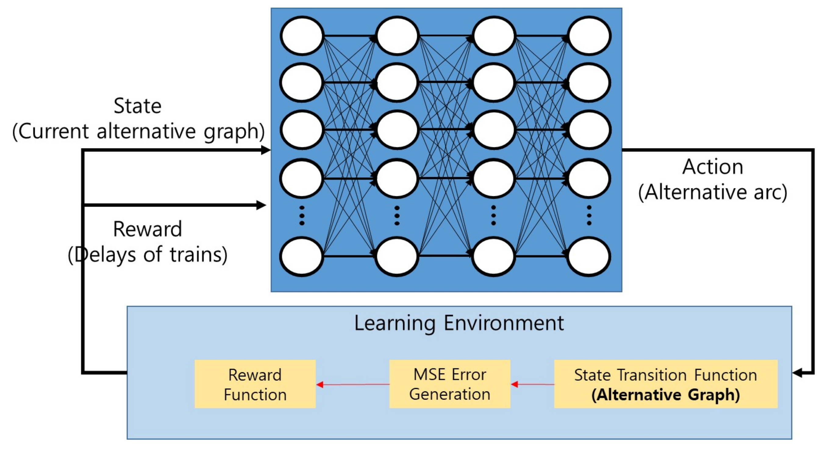
1.2. Preliminary: Reinforcement Learning

Many multi-stage or sequential decision problems can be formulated as interactions between the environment and agent (decision-maker). In these interactions, the information being used by the agent to make a decision is referred to as the state, and the agent receives a reward for his/her action (or decision) at a particular state. At the next decision time, the agent will encounter new information, which might depend on the previous state and action he/she chooses.

Generally, the next state of the environment depends on the entire history of pairs of states and actions. In the Markov decision process (MDP), however, it is assumed that the next state depends only on the current state and action. For a given MDP problem, Bellman optimality conditions [20] are usually derived, and the dynamic programming relying on these optimality conditions can be applied to find an optimal solution. Dynamic programming, however, is an enumerative solution approach that relies on searching for solutions in the entire solution space, such that it suffers from the so-called “curse of dimensionality” problem [21].

Reinforcement learning is one way to mitigate the computational limitations of an enumerative search of the solution space, by relaxing the goal of finding any exact optimal solutions. To do this, instead of searching all possible pairs of states and actions, a relatively small samples of states and actions is simulated and an optimal or near-optimal solution for the problem with respect to these samples is deduced. One of the central concepts in reinforcement learning is the optimal value function of a state, or pair of states, and an action, which specifies the long-term cumulative reward achievable when the agent follows (possibly unknown) an optimal decision after the given state or the given pair of states and action. For a given sample, we can estimate the optimal value function, and the estimated value function can be used directly or indirectly to specify the decisions the agent makes. In the recent development of reinforcement learning, deep neural networks [22] have been used for estimating the value function or a function, i.e., policy, which outputs an optimal action for a given state as an input, which achieves state-of-the-art results for many benchmark problems [23,24].

More background information on reinforcement learning can be found in [20,21].

2. Materials and Methods

Our objective is to find the selection S that represents a set of alternative arcs to minimize the train delays in a given alternative graph. The framework of the proposed model is presented in Figure 2. The proposed framework follows the general process of general reinforcement learning; however, it can be distinguished in two key aspects. Firstly, the agent of the proposed framework first obtains the information used in the state from the current alternative graph. Secondly, he/she executes state transitions by performing updates that involve adding the selected alternative arc to the alternative graph during the action phase.

The proposed method is applicable, in principle, given the availability of a physical railway network and timetable for the target railway lines. More specifically, it requires information on the connectivity between blocks and the expected arrival and departure times of trains for each block they traverse. Generally, train-operating companies maintain the real-time management of the aforementioned information at their control centers.

In the remaining part of this section, we present the rationale of our method. We first explain the proposed Markov decision process model of train conflict resolution based on the alternative graph. Then, we apply the method of deep Q-learning to find the optimal policy.

2.1. MDP Formulation

An alternative graph enables the detection of train conflict on a microscopic level, in addition to the ability to explicitly model the operation constraints such as the minimum speed, stop, and departure, and connections. As explained previously, the MDP model we propose interprets the train conflict resolution as sequential decision-making, in which an alternative arc is selected at each stage. Therefore, for each step t, it is required for the decision-maker, the agent in the MDP, to have information on all nodes and fixed arcs and the alternative arc up to step t. The size of the alternative graph changes, however, depending on the number of trains and their routes. Since the dimension or size of the state is assumed to be fixed, it is challenging to manage two different instances with different numbers of trains on the same railway network with a single policy. This suggests that we need a way to design the state of the MDP independent of the number of trains. To address this challenge, we introduce a mapping from train to block, denoted by $f_t:\mathcal{T}\to \mathcal{B}$ at decision step t. For each block $b\in \mathcal{B}$, let $f_t^{-1}\left(b\right)$ be the train on block b at decision step t.

Recall that the state space depicts the information given to the agent as the basis for decision-making regarding which action to select. In this respect, the state $s_t$ at decision step t is designed to consist of 12 features, as shown in

Table 1. Components of a state.

Features	Dimension	Type
The number of total trains ($NT$)	1	Static
Physical network ($PN$)	$\left|\mathcal{B}\right|\times \left|\mathcal{B}\right|$	Static
Junction indicator ($JI$)	$\left|\mathcal{B}\right|$	Static
Occupation indicator ($OI$)	$\left|\mathcal{B}\right|$	Dynamic
Next occupation indicator ($NI$)	$\left|\mathcal{B}\right|$	Dynamic
Upward direction ($UD$)	$\left|\mathcal{B}\right|$	Dynamic
Downward direction ($DD$)	$\left|\mathcal{B}\right|$	Dynamic
Occupation beginning time ($OB$)	$\left|\mathcal{B}\right|$	Dynamic
Occupation ending time ($OE$)	$\left|\mathcal{B}\right|$	Dynamic
AG node in-degree ($ID$)	$\left|\mathcal{B}\right|$	Dynamic
AG node out-degree ($OD$)	$\left|\mathcal{B}\right|$	Dynamic
AG cost ($AC$)	1	Dynamic

.

The components of the state are categorized into two types: static and dynamic. The number of total trains ($NT$), the physical network ($PN$) represented as a 0–1 adjacent matrix, and the junction indicator ($JI$) are of the static type. The physical network $P{N}_{ij}$ is 1 if blocks i and j are connected, or 0 otherwise. Junction indicator $J{I}_b$ is 1 if block b has a junction, or 0 otherwise.

For the dynamic type, occupation indicator $O{I}_b$ is 1 if block b is occupied by any train, or 0 otherwise. The next occupation indicator $N{I}_b$ is 1 if train $f_t^{-1}\left(b\right)$ could be moved to its next block at the next time step, or 0 otherwise. The upward (downward) direction $U{D}_b$ ($D{D}_b$) is 1 if the direction of the train $f_t^{-1}\left(b\right)$ is upward (downward), and is 0 otherwise. $O{B}_b$ and $O{E}_b$ are the beginning and ending time of occupation for a block b by train $f_t^{-1}\left(b\right)$, respectively. Next, the in-degree and out-degree of the alternative graph denoted by $I{D}_b$ and $O{D}_b$ with respect to block b is defined as the number of incoming or outgoing arcs to the nodes associated with block b in the alternative graph $\mathcal{G}\left(S\right)$, which can be computed as ${\sum }_{\{i:B(i)=b\}}{\sum }_{\{j:(j,i)\in \mathcal{F}\cup \mathcal{S}\}}{\delta }_{ji}$ and ${\sum }_{\{i:B(i)=b\}}{\sum }_{\{j:(i,j)\in \mathcal{F}\cup \mathcal{S}\}}{\delta }_{ij}$, respectively, where ${\delta }_{ij}$ or ${\delta }_{ji}$ equals 1 if arc (i, j) or (j, i) is contained in the alternative graph, and is 0 otherwise. Finally, $AC$ is defined as the longest path cost of the alternative graph $\mathcal{G}\left(S\right)$, denoted by $l^S(0,n)$. The values of the non-binary state are normalized to lie in $[0,1]$. More specifically, for each block $b\in \mathcal{B}$, we update $O{B}_b$, $O{E}_b$, $I{D}_b$, $O{D}_b$, and $AC$ to $\frac{O{B}_b}{{max}_{b\in \mathcal{B}}\left\{O{B}_b\right\}}$, $\frac{O{E}_b}{{max}_{b\in \mathcal{B}}\left\{O{E}_b\right\}}$, $\frac{I{D}_b}{{max}_{b\in \mathcal{B}}\{I{D}_b,O{D}_b\}}$, $\frac{O{D}_b}{{max}_{b\in \mathcal{B}}\{I{D}_b,O{D}_b\}}$, and $\frac{AC}{M}$, respectively, where M is a sufficiently large positive constant.

In short, state $s_t$ at step t is defined as

$$s_t=\left(NT,{\left\{\left(P{N}_{ij}\right)\right\}}_{i\in \mathcal{B},j\in \mathcal{B}},{\left\{(J{I}_b,O{I}_b,N{I}_b,U{D}_b,D{D}_b,O{B}_b,O{E}_b,I{D}_b,O{D}_b)\right\}}_{b\in \mathcal{B}},AC\right).$$

(6)

The size of state $s_t$ is ${\left|\mathcal{B}\right|}^2+9\left|\mathcal{B}\right|+2$, where $\left|\mathcal{B}\right|$ is the total number of blocks in the railway network.

For a given state $s_t$ at step t, the action $a_t$ chosen by the agent is interpreted as the choice of the alternative arc. More specifically, the choice of the alternative arc is defined as the choice of blocks that satisfies the following condition. Whenever the agent is requested, he/she chooses one of the available blocks, say b, which is currently occupied by a train, i.e., $O{I}_b=1$, and the next block $b^{\prime }$ of train $f_t^{-1}\left(b\right)$ is not occupied by any trains, i.e., $N{I}_{b^{\prime }}=1$. This means that the agent decides to move the train $f_t^{-1}\left(b\right)$ forward from block b to its next block $b^{\prime }$. Note that only one train can be selected to move at each step. If there is no available block for the action, then the agent selects the dummy action denoted by 0, and the episode is terminated. Therefore, the size of the possible action is $\left|B\right|+1$.

We proceed further with the alternative graph to select an action $a_t$ for the transition from the current state $s_t$ to the next state $s_{t+1}$. Whenever the agent is requested, he/she chooses one of the available blocks occupied by a train, i.e., $O{I}_b=1$, and the next block of $f_t^{-1}\left(b\right)$ not occupied by any trains, i.e., $N{I}_b=1$. Let $A\left(s_t\right)$ be the available action set at $s_t$. Action $a_t\in A\left(s_t\right)$ means that the agent decides to move the train $f_t^{-1}\left(a_t\right)$ forward from the current block $a_t$ to its next block ${a_t}^{\prime }$. Note that only one train is selected to move at each time step. If there is no available block, then the agent selects the dummy action denoted by 0 and the episode is terminated. Therefore, $\left|A\right(s_t\left)\right|$ is at most $\left|\mathcal{B}\right|+1$.

Once the agent determines the action $a_t$, we first find the corresponding train $f_t^{-1}\left(a_t\right)$ and the next block ${a_t}^{\prime }$; the train moves forward. If ${a_t}^{\prime }$ is used only by the train $f_t^{-1}\left(a_t\right)$, $\mathcal{G}\left(S\right)$ does not change, but the occupancy information of the next state $s_{t+1}$ only changes when the train $f_t^{-1}\left(a_t\right)$ moves forward one block.

If the next block ${a_t}^{\prime }$ is commonly used by more than one train, we can specify the alternative arcs that determine the occupancy order with other trains using ${a_t}^{\prime }$ in common. Then, the alternative arcs are added to selection S and the updated alternative graph $\mathcal{G}\left(S\right)$ is used for the next state $s_{t+1}$. More specifically, dynamic features are updated as follows: $O{B}_b=l^S(0,(f^{-1}\left(b\right),b))-(D_b^{f^{-1}\left(b\right)}-A_b^{f^{-1}\left(b\right)})$, $O{E}_b=l^S(0,(f^{-1}\left(b\right),b))$, and $AC=l^S(0,n)$.

The reward function plays the role of directing the agent’s behavior toward the optimal policy. Recall that the goal of TTR is to minimize the length of the longest path from Node 0 to node n in the alternative graph by choosing the alternative arcs. Since the length of the longest path is finally determined when the dummy action is chosen, we define the reward $r_t$ at each step t as follows:

$$r_t=\left\{\begin{array}{cc}\hfill 0,\hfill & \hfill a_t\in \mathcal{B}\hfill \\ \hfill -l^S(0,n),\hfill & \hfill a_t=0.\hfill \end{array}\right.$$

(7)

By setting the reward $r_t$ as the negative value of $l^S(0,n)$ when $a_t=0$, maximizing the cumulative total reward is identical to minimizing $l^S(0,n)$. If the graph $\mathcal{G}\left(S\right)$ has positive length cycles, we define $l^S(0,n)$ as M, a sufficiently large positive constant.

Example 1.

In this subsection, we illustrate the corresponding MDP model in Figure 1. We assume that the weights of all fixed and alternative arcs are 5 and 2, respectively. First, the static features are defined as follows:

$$PN=\left(\begin{array}{ccccc}0& 0& 1& 0& 0\\ 0& 0& 1& 0& 0\\ 1& 1& 0& 1& 0\\ 0& 0& 1& 0& 1\\ 0& 0& 0& 1& 0\end{array}\right),\mathit{and}JI=(0,0,1,0,0).$$

Then, we consider the dynamic features. At the beginning, dynamic features (features in Table 1 types as “dynamic”) of $s_0$ are constructed by concatenating $OI=(1,1,0,0,0)$, $NI=(1,1,0,0,0)$, $UD=(1,1,0,0,0)$, $DD=(0,0,0,0,0)$, $OB=(0,0,0,0,0)$, $OE=(5/5,5/5,0,0,0)$, $ID=(1/2,1/2,2/2,2/2,2/2)$, $OD=(1/2,1/2,2/2,2/2,2/2)$, and $AC=\frac{20}{M}$. The legitimate actions correspond to Block 1 and Block 2. If the agent selects action 1, then Train A moves forward, from Block 1 to Block 3. This implies that the alternative arc $\left(\right(A,3),(B,2\left)\right)$ is added to the current selection S, as illustrated in Figure 3a. If the agent selects Action 2, then Train B moves from Block 2 to Block 3, which implies the addition of the alternative arc $\left(\right(B,3),(A,1\left)\right)$ to S.

At $t=1$, the dynamic features of $s_1$ are updated as follows: $OI=(0,1,1,0,0)$, $NI=(0,0,1,0,0)$, $UD=(0,1,1,0,0)$, $DD=(0,0,0,0,0)$, $OB=(0,7/12,5/12,0,0)$, $OE=(0,12/12,10/12,0,0)$, $ID=(1/3,2/3,2/3,2/3,2/3)$, $OD=(1/3,1/3,3/3,2/3,2/3)$, and $AC=\frac{27}{M}$. Then, the only legitimate action corresponds to block 3, i.e., $O{I}_3=1$ and $N{I}_3=1$. Therefore, we add the alternative arc $\left(\right(A,4),(B,3\left)\right)$ to the current selection S. Figure 3b shows the block occupation and alternative graph at $t=1$.

2.2. Deep Q-Learning

In reinforcement learning, instead of directly considering policies, a policy can be derived from the so-called action value function or the Q-value function. For each policy $\pi$, the action value function $Q_{\pi }(s_t,a_t)$ is the expected total return given an action $a_t$ at state $s_t$ assuming the agent follows the policy $\pi$. The optimal action value function is then defined as $Q_{*}(s_t,a_t)={max}_{\pi }(s_t,a_t)$.

Q-learning [25] maintains a lookup table of $Q(s,a)$ for every state–action pair $(s,a)$. To estimate the optimal action-value function $Q^{*}(s,a)$, the Q-learning approach uses the following updates:

$$Q(s,a)\leftarrow Q(s,a)+\alpha \left(r_t+\gamma \underset{a_{t+1}}{max}Q(s_{t+1},a_{t+1})-Q(s_t,a_t))\right)$$

(8)

where $\alpha \in [0,1]$ is the learning rate.

However, Q-learning suffers the curse of dimensionality in maintaining the look-up table when the number of states and/or actions is large. One way to address this challenge is to approximate the Q-value function as a neural network. In particular, Mnih et al. [26] proposed the DQN method, which uses a deep neural network as a function approximation of the Q-value function. The neural network, called the deep Q-network, is modeled as a parameterized function $Q(s_t,a_t|\theta )$ and is determined by adjusting the parameter $\theta$ in the direction of minimizing the following loss function:

$$L\left(\theta \right):={\left(\left[r_t+\gamma \underset{a_{t+1}}{max}Q(s_{t+1},a_{t+1}|\theta )\right]-Q(s_t,a_t|\theta )\right)}^2.$$

(9)

To learn the optimal parameters and scenarios, the alternate sequences of states, actions, and rewards are randomly generated. To generate each scenario, an action is chosen from the current state $s_t$ via the $ϵ$-greedy policy in which the agent chooses the action maximizing the $Q(a,s_t)$, but there exists a small chance that $ϵ$ will choose a random action. In this way, we obtain a set of $(s_t,a_t,r_t,s_{t+1})$, which constitutes the loss function $L\left(\theta \right)$. The trained Q-network is used to make a decision by selecting the action that maximizes the Q-value. The pseudocode of the training phase of the proposed method is shown in Algorithm 1.

Algorithm 1: Train timetable rescheduling with Q-network.

Input: Alternative graph $\mathcal{G}=(\mathcal{N},\mathcal{F})$

Output: Q-network, selection S

In Algorithm 1, to mitigate the issue of instabilities during learning, the following techniques are typically incorporated [26]:

• Experience replay: In its basic setting, Q-learning is on-policy, which means we generate scenarios and learn parameters simultaneously. When we consider the loss function with $(s_t,a_t,r_t,s_{t+1})$ obtained from a set of scenarios, there exists autocorrelation among different $(s_t,a_t,r_t,s_{t+1})$. However, most algorithms used for training deep neural networks assume that training samples are independently and identically distributed. Therefore, instead of on-policy learning, off-policy learning is incorporated, in which $(s_t,a_t,r_t,s_{t+1})$ is stored in the so-called replay memory and a minibatch of a set of random samples from this memory forms the loss function.
• Target network: In both Q-learning and deep Q-learning, scenarios are generated with the policy derived by the current Q-value function being updated. This has been identified as one of the reasons for unstable learning. To overcome this problem, Mnih et al. [26] used two separate neural networks, $Q(s_t,a_t|\theta )$ and $Q^{\prime }(s_t,a_t|{\theta }^{\prime })$. The former network is used to generate random scenarios, and the latter, called the target network, is used to set the target in the loss function $L\left(\theta \right)$. The parameter $\theta$ is updated in the same way introduced previously, and the parameter ${\theta }^{\prime }$ of the target network is kept unchanged during a predefined number of steps and updated to the parameter $\theta$.

3. Experimental Results

This section reports the computational results obtained by applying the approaches in Section 2. All codes were implemented in the Python language. In particular, the neural network and its training algorithm were implemented in the Keras library with the TensorFlow backend. All experiments were performed with a personal computer with an Intel Core TM i7-12700 CPU processor (2.1 GHz). In

Table 2. Hyperparameters for the DQN agent.

Hyperparameters	Values
The number of hidden layers	4
The numbers of nodes in each hidden layer	1024, 512, 256, 128
Decay factor of $ϵ$ per episode	0.9999
Replay buffer size	20,000,000
Minibatch size	256
Discount factor	0.9
Target Q-network update frequency	16
M	99,999

, we summarize the hyperparameters for the DQN agent introduced in Section 2.2.

The performance of the proposed DQN was compared with an exact method, the MILP model in Section 1.1, by applying the commercial software package GUROBI 10.0.2. The performance of each solution approach was evaluated via GAP, defined as

$$\mathrm{GAP}=\frac{\mathrm{DQN}-\mathrm{MILP}}{\mathrm{MILP}}\times 100.$$

(10)

where “DQN” and “MILP” denote the $l^S(0,n)$ value obtained from the trainedagent (DQN) and the optimum value of the MILP model, respectively.

In order to evaluate the performance of the DQN agent, experiments were carried out on a simple and complex network. First, we trained and tested our model on the simple railway network proposed in [27]. Next, the performance was evaluated for the study area inside Seoul station in Korea.

3.1. Results on a Simple Network

Figure 4 shows a simple railway network with 10 blocks (denoted as 1, 2, …, 10) and three trains (denoted as A, B, and C). Train A enters from Block 1 and exits from Block 10, passing through Blocks 2, 3, 5, 6, and 8. Train B travels from Block 9 to Block 1, passing through Blocks 8, 6, 5, 4, and 2. Similarly, Train C enters from Block 7 and exits to Block 1, passing through Blocks 6, 5, 4, and 2. We set the travel time of each block as 300 s, except Blocks 3 and 4, which were platforms in the station that each required 420 s. The safety headway between two consecutive trains on each block was set to 120 s, including switching and signaling time. Therefore, the weight of all alternative arcs was 120 s.

All trains were scheduled to arrive at their entry blocks at 07:00:00. To train a Q-network, the entry delay time of each train was randomly generated from a uniform distribution [0, U] in seconds and added to the planned times for each episode. This enables the trained Q-network to accommodate the various train rescheduling problems in the training phase. In Figure 5, we present the convergence performance for up to 48,000 episodes with $U=600$ in the training phase. In the plots shown in Figure 5, the x and y axes indicate the cumulative number of episodes and the simple moving average of the previous 100 reward values, respectively. As shown in Figure 5, fluctuations caused by the $ϵ$-greedy policy were observed.

We performed testing on the generated instances with respect to the maximum entry delay time ($U=\{300,600,900,1200\}$). We generated 100 instances for each U, and thus, a total 400 instances were tested.

Table 3. Average runtime and GAP values for instances of a simple network.

U	MILP		DQN
	# of Optimal	Avg. Runtime	# of Optimal	Avg. Runtime	Avg. GAP
300	100	0.005 s	100	0.740 s	0.00
600	100	0.005 s	93	0.747 s	0.01
900	100	0.005 s	80	0.744 s	0.14
1200	100	0.005 s	71	0.770 s	0.25

summarizes the performance of the DQN with respect to three dimensions: the number of instances finding an optimal solution, the average CPU runtime (in seconds), and the average GAP value obtained by Equation (10). Column 1 indicates the category of instances; Columns 2–3 contain the performance of the exact method; Columns 4–6 report the performance of the DQN. The exact method finds the optimal solutions for all instances in 0.005 s. Tested on instances with $U=300$, the DQN also finds the optimal solutions for all instances, although it takes more time to compute the solutions. The number of times that DQN finds the optimal solution decreases to 93, 80, and 71 when $U=600$, $U=900$, and $U=1200$, respectively. However, the GAP values are less than 0.25% on average, and the runtime of the DQN does not vary significantly.

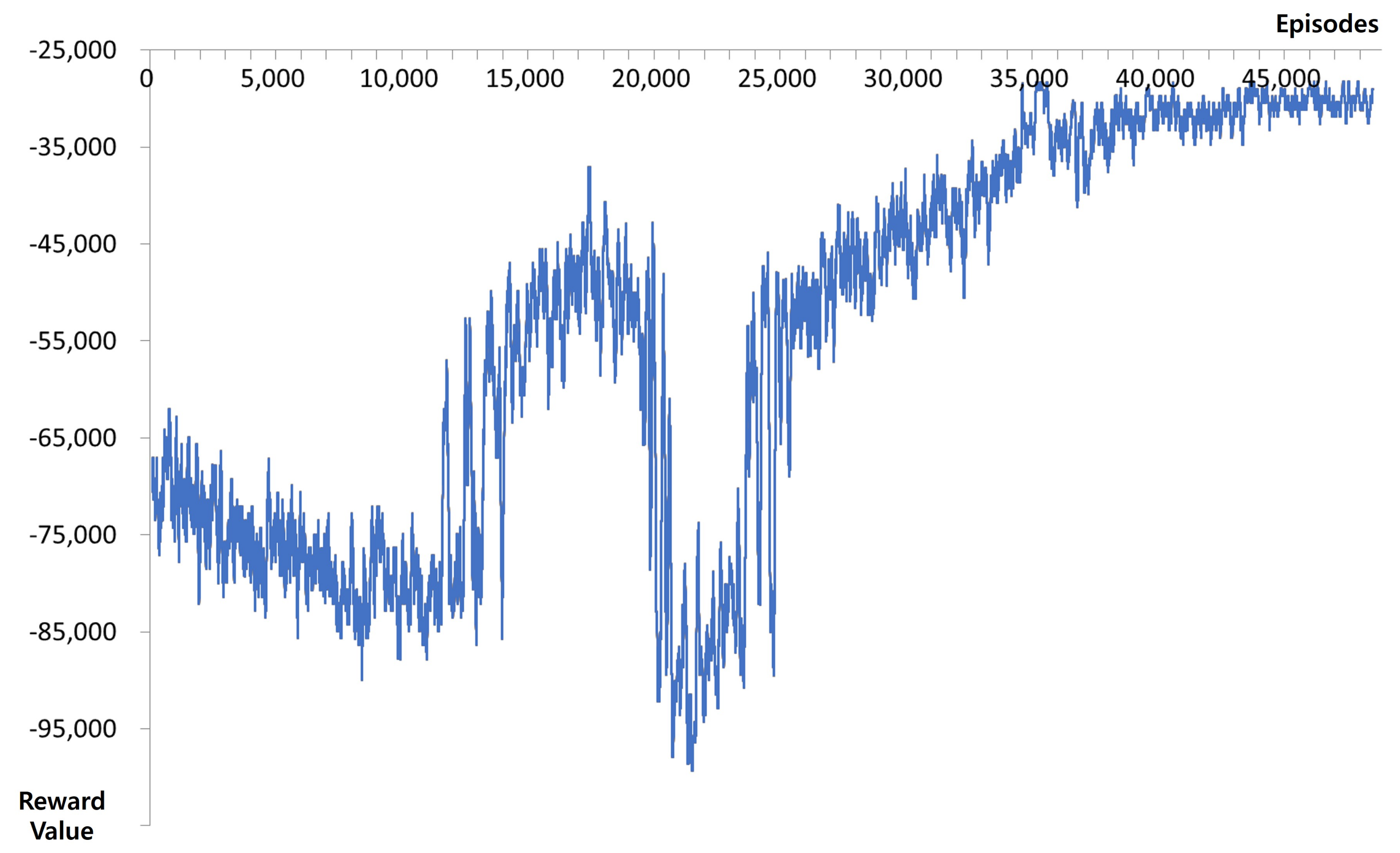
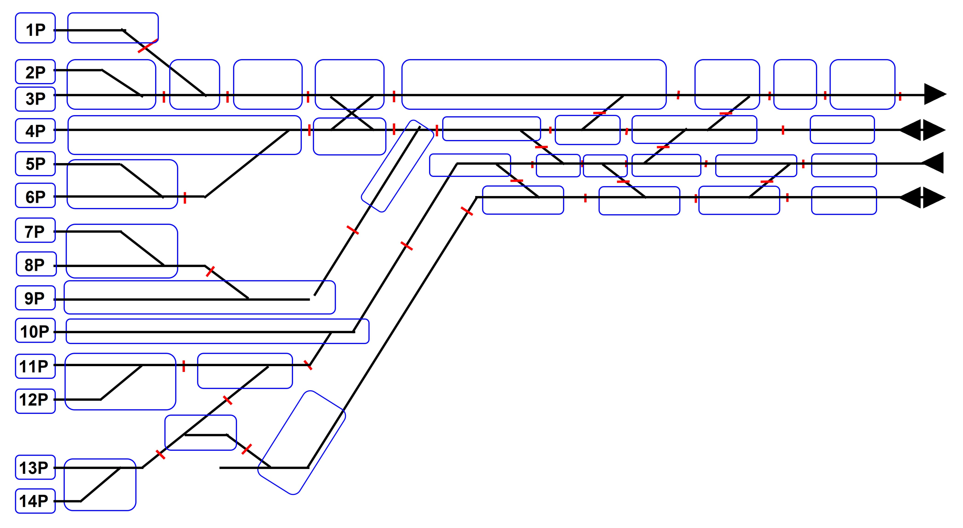
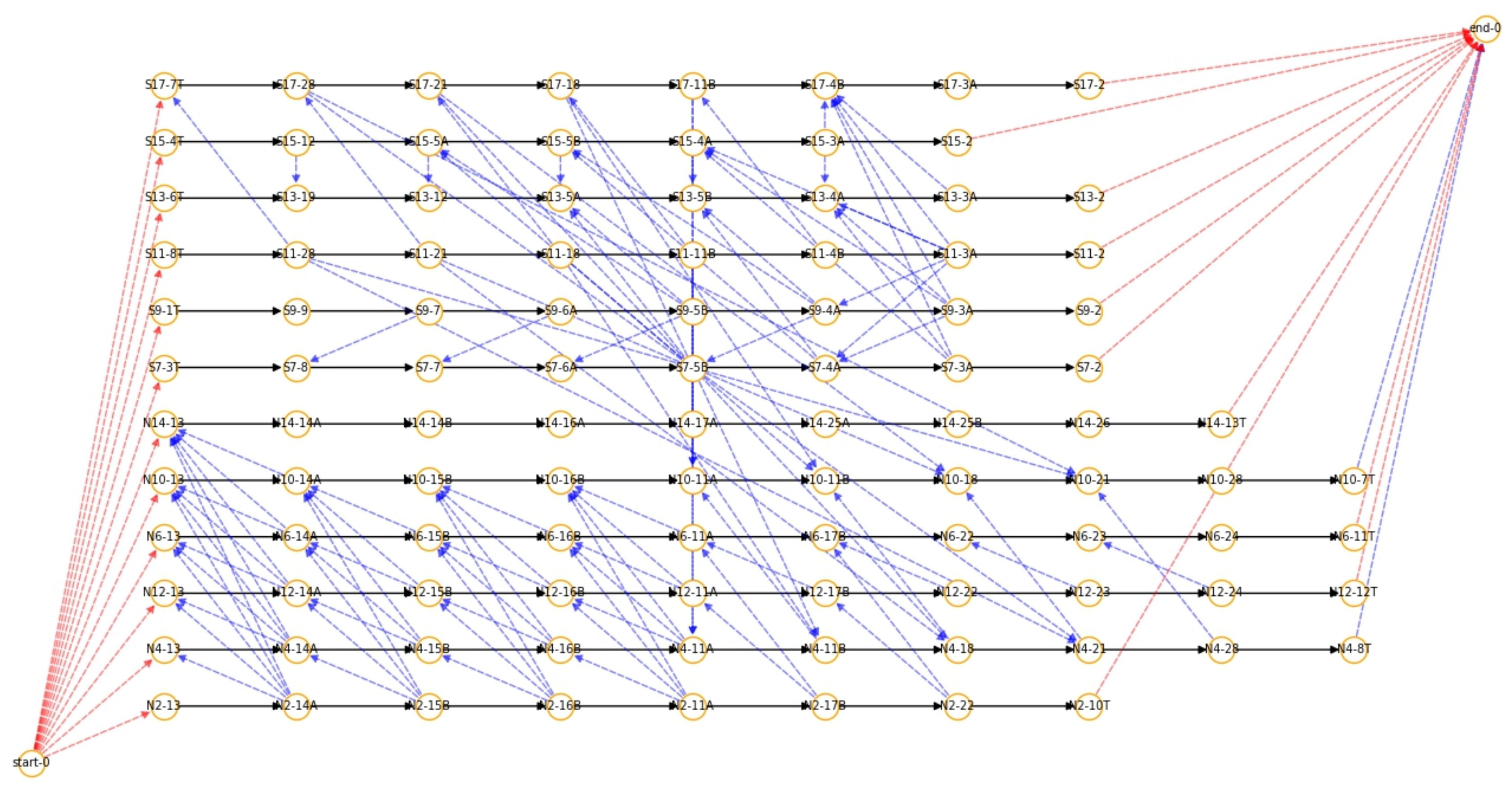
3.2. Results for Seoul Station

The performance of the RL was tested in the Seoul station area, as shown in Figure 6. This area consists of 49 blocks, containing 29 junctions and 14 platforms, making it currently the most-complex area in Korea. The network was considered with microscopic detail, considering switches, signals, etc. In the actual train timetable, there are 12 trains driving on this network between 7 a.m. and 8 a.m. Therefore, the DQN was trained using these 12 trains with uniform entry delay time [0, 600]. The DQN was tested on these instances, varying the maximum entry delay time and the number of trains, denoted as $U=\{300,600,900,1200\}$ and $NT=\{10,12,14,16,18\}$, respectively. We generated 100 instances for each category, denoted (U, $NT$). Therefore, a total of 2000 instances were tested. Note that we forced our DQN to face novel scenarios by increasing the number of trains with different departure times or destination platforms compared with those of previous trains.

Figure 7 shows the alternative graph with a feasible selection obtained by the DQN for an instance with (300, 12). The fixed arcs generated by 12 trains are indicated as black bold arrows, and 125 alternative arcs are indicated as blue dashed arrows. Lastly, red dashed arrows indicate edges connected to two dummy nodes: entry and exit.

Table 4. Average runtime and GAP values for instances at Seoul station.

(U, $\mathbf{NT}$)	MILP		DQN
	# of Optimal	Avg. Runtime	# of Optimal	Avg. Runtime	Avg. GAP
(300, 10)	100	0.035 s	82	4.582 s	0.04
(300, 12)	100	0.043 s	100	5.020 s	0.00
(300, 14)	100	0.061 s	100	6.268 s	0.00
(300, 16)	100	0.077 s	100	7.083 s	0.00
(300, 18)	100	0.091 s	100	8.005 s	0.00
(600, 10)	100	0.035 s	75	4.543 s	0.11
(600, 12)	100	0.042 s	100	5.154 s	0.00
(600, 14)	100	0.054 s	98	5.818 s	0.00
(600, 16)	100	0.069 s	94	6.669 s	0.01
(600, 18)	100	0.078 s	100	7.498 s	0.00
(900, 10)	100	0.033 s	58	4.278 s	0.25
(900, 12)	100	0.044 s	100	5.182 s	0.00
(900, 14)	100	0.057 s	93	5.957 s	0.02
(900, 16)	100	0.067 s	87	6.645 s	0.05
(900, 18)	100	0.078 s	98	7.354 s	0.00
(1200, 10)	100	0.031 s	71	4.019 s	0.23
(1200, 12)	100	0.044 s	98	5.180 s	0.01
(1200, 14)	100	0.051 s	85	5.619 s	0.10
(1200, 16)	100	0.063 s	81	6.352 s	0.07
(1200, 18)	100	0.073 s	88	7.184 s	0.06

summarizes the comparisons of MILP and the DQN with respect to three dimensions: number of instances that succeed in finding an optimal solution, average runtime, and average GAP values. Tested on instances with $U=300$, the MILP model finds optimal solutions for all instances, and the average CPU times tend to increase with respect to the number of trains. The DQN also succeeds in finding an optimal solution for all instances except for $NT=10$.

Tested on instances with $U=600$, the MILP model showed similar results for the instances with $U=300$. The DQN failed to find the optimal solutions for all instances except for $NT=12$ and $NT=18$. However, the GAP values were less than 0.11, which shows that the quality of solutions was comparable to that of the exact method. Tested on instances with $U=900$ and $U=1200$, the GAP values obtained by the DQN were maintained under 0.10 for all instances except for $NT=10$. However, by increasing the value of U, the average number of instances to obtain the optimal solution decreased from 96.7 in $U=300$ to 88.5 in $U=1200$.

Overall, the experiments carried out using real-world cases showed that the performance of the exact method was superior to that of the proposed DQN with respect to the quality of solutions and the computation time. However, the increasing rate of the computation time of the DQN was significantly less than that of MILP with respect to the increase in the number of trains. One of the advantages of the DQN is that it shows great scalability. Furthermore, considering the extension and generalization of the problem, such as including nonlinear terms in the objective and/or constraints, the proposed DQN represents a practical method to replace the exact method based on the MILP model on complex railway networks with high traffic density.

4. Conclusions and Discussion

This paper considered a train timetable rescheduling problem at the microscopic level using an alternative graph model. The objective was to minimize the maximum consecutive delay, expressed as the cost of the longest path on an alternative graph.

First, we developed a Markov decision process model with an alternative graph model. This enabled us to more explicitly handle various operational constraints without a train operation simulator. In addition, the state of the MDP was designed to be independent of train operation planning, which makes the proposed MDP more applicable to diverse instances. Then, the proposed model was tested on a simple, real-world railway network in the Seoul station area. By evaluating the performance of the DQN through numerical experiments, we concluded that the proposed DQN is comparable to exact methods based on the MILP model with respect to the quality of the solutions. However, the computation time needs to be further improved.

Reinforcement learning issues arise in almost every area of railway operation: train timetabling, trajectory optimization, and control equipment such as the pantograph. MDP-based reinforcement learning using the alternative graph model is a potential area of study for train dispatch or conflict resolution algorithms. Obtaining actual train operation data is exceedingly challenging. Therefore, in order to generate training data using train operation simulators such as OpenTrack, significant costs and time are required, including the implementation of the APIs. We observed that the alternative graph model can potentially replace train operation simulators and facilitate the more-convenient collection of microscopic-level training data. The computational complexity of the proposed method is proportional to the size of the alternative graph and, more specifically, the number of alternative arcs. These findings suggest that timetable rescheduling requires an MDP model that implements immediate selection, as proposed by [4] for computational complexity.

In this paper, similar to previous papers [11,12,13,14,15], the reinforcement learning model was assumed to be a DQN model. For future work, it would be interesting to find more proper alternative reinforcement learning models, such as the deep deterministic policy gradient (DDPG) employed by [28].

References

1. Cacchiani, V.; Huisman, D.; Kidd, M.; Kroon, L.; Toth, P.; Veelenturf, L.; Wagenaar, J. An overview of recovery models and algorithms for real-time railway rescheduling. Transp. Res. Part B Methodol. 2014, 63, 15–37. [Google Scholar] [CrossRef]
2. Min, Y.H.; Park, M.J.; Hong, S.P.; Hong, S.H. An appraisal of a column-generation-based algorithm for centralized train-conflict resolution on a metropolitan railway network. Transp. Res. Part B 2011, 45, 409–429. [Google Scholar] [CrossRef]
3. Törnquist, J.; Persson, J.A. N-tracked railway traffic re-scheduling during disturbances. Transp. Res. Part B 2007, 41, 342–362. [Google Scholar] [CrossRef]
4. Mascis, A.; Pacciarelli, D. Job-shop scheduling with blocking and no-wait constraints. Eur. J. Oper. Res. 2002, 143, 498–517. [Google Scholar] [CrossRef]
5. Mazzarello, M.; Ottaviani, E. A traffic management system for real-time traffic optimisation in railways. Transp. Res. Part B Methodol. 2007, 41, 246–274. [Google Scholar] [CrossRef]
6. D’Ariano, A.; Corman, F.; Pacciarelli, D.; Pranzo, M. Reordering and local rerouting strategies to manage train traffic in real time. Transp. Sci. 2008, 42, 405–419. [Google Scholar] [CrossRef]
7. D’ariano, A.; Pacciarelli, D.; Pranzo, M. A branch and bound algorithm for scheduling trains in a railway network. Eur. J. Oper. Res. 2007, 183, 643–657. [Google Scholar] [CrossRef]
8. Mannino, C.; Mascis, A. Optimal real-time traffic control in metro stations. Oper. Res. 2009, 57, 1026–1039. [Google Scholar] [CrossRef]
9. Lamorgese, L.; Mannino, C. An exact decomposition approach for the real-time train dispatching problem. Oper. Res. 2015, 63, 48–64. [Google Scholar] [CrossRef]
10. Corman, F.; D’Ariano, A.; Pacciarelli, D.; Pranzo, M. Dispatching and coordination in multi-area railway traffic management. Comput. Oper. Res. 2014, 44, 146–160. [Google Scholar] [CrossRef]
11. Šemrov, D.; Marsetič, R.; Žura, M.; Todorovski, L.; Srdic, A. Reinforcement learning approach for train rescheduling on a single-track railway. Transp. Res. Part B Methodol. 2016, 86, 250–267. [Google Scholar] [CrossRef]
12. Khadilkar, H. A Scalable Reinforcement Learning Algorithm for Scheduling Railway Lines. IEEE Trans. Intell. Transp. Syst. 2019, 20, 727–736. [Google Scholar] [CrossRef]
13. Ning, L.; Li, Y.; Zhou, M.; Song, H.; Dong, H. A deep reinforcement learning approach to high-speed train timetable rescheduling under disturbances. In Proceedings of the 2019 IEEE Intelligent Transportation Systems Conference (ITSC), Auckland, New Zealand, 27–30 October 2019; pp. 3469–3474. [Google Scholar]
14. Zhu, Y.; Wang, H.; Goverde, R.M. Reinforcement learning in railway timetable rescheduling. In Proceedings of the 2020 IEEE 23rd International Conference on Intelligent Transportation Systems (ITSC), Rhodes, Greece, 20–23 September 2020; pp. 1–6. [Google Scholar]
15. Gong, I.; Oh, S.; Min, Y. Train scheduling with deep Q-Network: A feasibility test. Appl. Sci. 2020, 10, 8367. [Google Scholar] [CrossRef]
16. Agasucci, V.; Grani, G.; Lamorgese, L. Solving the train dispatching problem via deep reinforcement learning. J. Rail Transp. Plan. Manag. 2023, 26, 100394. [Google Scholar] [CrossRef]
17. Shuo Ying, C.; Chow, A.H.; Nguyen, H.T.; Chin, K.S. Multi-agent deep reinforcement learning for adaptive coordinated metro service operations with flexible train composition. Transp. Res. Part B Methodol. 2022, 161, 36–59. [Google Scholar] [CrossRef]
18. Li, W.; Ni, S. Train timetabling with the general learning environment and multi-agent deep reinforcement learning. Transp. Res. Part B Methodol. 2022, 157, 230–251. [Google Scholar] [CrossRef]
19. Lamorgese, L.; Mannino, C.; Pacciarelli, D.; Krasemann, J.T. Train dispatching. In Handbook of Optimization in the Railway Industry; Springer: Berlin/Heidelberg, Germany, 2018; pp. 265–283. [Google Scholar]
20. Sutton, R.S.; Barto, A.G. Reinforcement Learning: An Introduction; The MIT Press: London, UK, 2020. [Google Scholar]
21. Powell, W.B. Approximate Dynamic Programming: Solving the Curses of Dimensionality; John Wiley & Sons: Hoboken, NJ, USA, 2007. [Google Scholar]
22. Goodfellow, I.; Bengio, Y.; Courville, A. Deep Learning; The MIT Press: London, UK, 2016. [Google Scholar]
23. Arulkumaran, K.; Deisenroth, M.P.; Brundage, M.; Bharath, A.A. Deep Reinforcement Learning: A Brief Survey. IEEE Signal Process. Mag. 2017, 34, 26–38. [Google Scholar] [CrossRef]
24. Wang, X.; Wang, S.; Liang, X.; Zhao, D.; Huang, J.; Xu, X.; Dai, B.; Miao, Q. Deep Reinforcement Learning: A Survey. IEEE Trans. Neural Netw. Learn. Syst. 2022, 1–15. [Google Scholar] [CrossRef] [PubMed]
25. Watkins, C.; Dayan, P. Q-learning. Mach. Learn. 1992, 8, 279–292. [Google Scholar] [CrossRef]
26. Mnih, V.; Kavukcuoglu, K.; Silver, D.; Rusu, A.; Veness, J.; Bellemare, M.; Graves, A.; Riedmiller, M.; Fidjeland, A.; Ostrovski, G.; et al. Human-level control through deep reinforcement learning. Nature 2015, 518, 529–533. [Google Scholar] [CrossRef] [PubMed]
27. Pacciarelli, D. Deliverable D3: Traffic Regulation and Co-operation Methodologies-code WP4UR_DV_7001_D. In Proj. COMBINE 2 “Enhanced COntrol Centres Fixed Mov. Block SIgNalling SystEms-2” Number: IST-2001-34705; 2003. [Google Scholar]
28. Shuo Ying, C.; Chow, A.H.; Chin, K.S. An actor-critic deep reinforcement learning approach for metro train scheduling with rolling stock circulation under stochastic demand. Transp. Res. Part B Methodol. 2020, 140, 210–235. [Google Scholar] [CrossRef]
Figure 1. Example railway network, trains, and alternative graph.
Applsci 13 09547 g001
Figure 2. Overview of framework for reinforcement learning.
Applsci 13 09547 g002
Figure 3. (a) Example of state transition at t = 0 ; (b) Example of state transition at t = 1 .
Applsci 13 09547 g003
Figure 4. Simple network.
Applsci 13 09547 g004
Figure 5. Training results with respect to the cumulative number of episodes with U = 600 .
Applsci 13 09547 g005
Figure 6. Seoul station railway network.
Applsci 13 09547 g006
Figure 7. Feasible selection and its alternative graph obtained by the DQN for an instance with (300, 12).
Applsci 13 09547 g007