Battery State Estimation with ANN and SVR Evaluating Electrochemical Impedance Spectra Generalizing DC Currents

Abstract

The demand for energy storage is increasing massively due to the electrification of transport and the expansion of renewable energies. Current battery technologies cannot satisfy this growing demand as they are difficult to recycle, as the necessary raw materials are mined under precarious conditions, and as the energy density is insufficient. Metal–air batteries offer a high energy density as there is only one active mass inside the cell and the cathodic reaction uses the ambient air. Various metals can be used, but zinc is very promising due to its disposability and non-toxic behavior, and as operation as a secondary cell is possible. Typical characteristics of zinc–air batteries are flat charge and discharge curves. On the one hand, this is an advantage for the subsequent power electronics, which can be optimized for smaller and constant voltage ranges. On the other hand, the state determination of the system becomes more complex, as the voltage level is not sufficient to determine the state of the battery. In this context, electrochemical impedance spectroscopy is a promising candidate as the resulting impedance spectra depend on the state of charge, working point, state of aging, and temperature. Previous approaches require a fixed operating state of the cell while impedance measurements are being performed. In this publication, electrochemical impedance spectroscopy is therefore combined with various machine learning techniques to also determine successfully the state of charge during charging of the cell at non-fixed charging currents.

1. Motivation

1.1. Importance of Battery Technology

The general sales volume of device batteries in Germany for all battery technologies is shown in Figure 1. A rapidly increasing trend can be seen. Currently, the lithium-ion technology is the most widely used, which were first brought to market by Sony in 1991. It offers high energy density and low weight. Another advantage is durability, as the technology is not based on the electrode material dissolving chemical reactions, but on the flow of lithium-ions between the anode and cathode. Lithium-ion batteries initially powered mainly portable devices with high energy requirements for which conventional nickel-cadmium or NiMH batteries were too heavy or too large. Now, they also serve as energy storage for pedelecs, modern electric wheelchairs, and PHEV.

This trend is not expected to slow down, as topics such as the digitization of industry, ubiquitous computing, and the IoT are only on the rise. Industry 4.0 is the name given to a future project for the comprehensive digitization of industrial production [2]. Depending on the size, location, and type of production facility, the requirements may only be possible with the help of battery-powered sensors and devices, as well as with energy-autonomous systems that require a buffer battery.

However, digitization is also taking place in areas outside industry. Battery electric vehicles (BEV) are the largest growth market for rechargeable batteries. Currently, the transportation sector within the EU is still largely based on fossil fuels and is responsible for more than 25% of Europe’s greenhouse gas emissions. Excluding the COVID-19 crisis, this share is even growing [3]. In addition to global warming, vehicles with combustion engines also form a significant part contributing to air pollution. In particular, the proportion of particulate matter and nitrogen dioxide increases as a result of combustion engines [3]. Electrified or partially electrified vehicles can help here. The level of greenhouse gas emissions over the entire vehicle life cycle depends to a large extent on the CO₂ balance of the generated electricity [3]. Even in the case of combustion vehicles, partial electrification in the form of a PHEV in combination with a battery can lead to an improvement in the environmental balance. Together with a falling price, this is leading to an increase in BEVs around the world, as can be seen in Figure 2. Furthermore, the demand for battery capacity and the raw materials is also growing massively. As electric cars mainly use lithium-ion cells, the demand for cobalt in particular is considered critical. This is as, as with many other ores, mining is partly carried out under precarious conditions, so that alternative battery technologies have to be used.

The environmental footprint of BEV is particularly good when renewable electricity is used to charge the electric cars. Renewable energy sources are energy sources that are practically inexhaustible in the horizon of mankind for sustainable energy supply or are renewed relatively quickly [5,6]. Uranium and other nuclear fuels are also finite, so nuclear energy is not an alternative to fossil fuels due to limited resources [6]. Therefore, a sustainable energy policy must rely on biomass, geothermal energy, hydro power, ocean energy, solar energy, and wind energy.

As renewable energies are to a large extent not permanently available and depend, for example, on the weather, grid stability must also be considered when expanding renewable energies. For example, the locations and technical characteristics of the plants influence grid stability, as does the quality of the grid. In addition, grid stability depends on the respective short-term power flows in the power grid, which in turn depend heavily on the weather in a renewable power supply. The grid is considered stable when frequency, voltage, and angular stability are satisfied.

While voltage stability can be maintained by distributed generation facilities and communication systems, maintaining frequency stability is more complex. To date, the rotating masses of the power generators support the grid frequency in the first moments of a power loss (frequency-response reserve). Such a power deficit can occur, for example, due to the failure of an offshore wind farm. The foreseeable absence of rotating masses raises the question of whether there will be sufficient frequency-response reserve in the power system in the future, or whether the system will have sufficient inertia in the event of abrupt power plant or line failures to allow sufficient time for the deployment of spinning reserve [7,8].

If the mismatch between consumed and generated energy exceeds the time horizon of the frequency response reserve, primary control power is used to ensure that frequency stability is not affected. If the energy demand is higher than predicted, power plants already in use are first operated at a higher working point and, if necessary, additional power plants that are in standby mode are brought online. The demand for control power that needs to be held in reserve increases with the increasing amount of weather-dependent renewable energies, whose output can only be predicted to a certain extent [9]. In principle, the possible power gradients of weather-dependent solar and wind power plants are sufficient to react quickly compared to large power plants. However, it should be noted that the availability of control power is only possible if there is sufficient wind or sun. As the allocation of control power by weather-dependent renewable energies is only possible by throttling, free available energy remains unused, which applies to the allocation of negative and positive control power. In the case of positive control power, however, the extent is greater, as the plants must be permanently throttled in order to be able to increase output if necessary [7].

Hence, for a complete roll-out of renewable energies, alternatives for power control must also be considered in order to ensure a safe system state of the grid. Due to the fast activation and reaction time, battery systems are ideal for providing the necessary control power. The time required to provide or consume energy is mainly determined by the used power electronics and reaches full load in the range of 20 $\mathrm{m}$$\mathrm{s}$. This means that battery systems can provide both frequency response reserve and operating reserve. To a certain extent, it is even possible to generate the replacement reserve with batteries. Therefore, the energy transition can only be achieved by a massive expansion of battery storage power plants. Already today, battery storage power plants are used to a significant extent. For example, in 2017, about 700 battery storage power plants with a capacity of over $2.5$ $\mathrm{G}$$\mathrm{W}$ were in operation. The majority of these use lithium-ion batteries with the problems already described [10].

1.2. Benefits of Zinc–Air Batteries

As already explained in the previous section, lithium-ion accumulators are currently used in numerous battery applications. Especially when considering the further storage demand due to electromobility and the expansion of renewable energies, a shortage of the necessary cell materials is expected. In particular, cobalt, which is used for the production of the positive electrode, is only available on a small scale on earth and has a high toxicity. The problem is further intensified by the fact that the majority of cobalt deposits are located in countries with poor working conditions, making it difficult to switch to other suppliers.

Zinc is a relatively frequent element on Earth, representing 76 ppm of the Earth’s crust, making it the 24th most frequent element [11]. It is thus more common than lithium (60 ppm), cobalt (40 ppm), or lead (18 ppm) [11,12,13]. Consequently, the price of zinc per ton is much lower than that of lithium [14]. In addition, the deposits are distributed all over the world, so that better working conditions can be guaranteed. Large deposits exist in the United States, Canada, Australia, and China, but there are also zinc deposits in Europe that are being actively mined [11]. Another major advantage of zinc is that it is completely recyclable. For example, it is estimated that in North America more than 33% of the utilized zinc is made from recycled materials. Globally, the recycling rate is about 40% of the produced zinc, with the recycling loops in Europe being largely closed for zinc recycling.

Further advantages of metal–air batteries, and thus of zinc–air batteries, are particularly high theoretical specific energies and theoretical energy densities [15,16]. The theoretical specific energy is given by Equation (1).

$$e=\frac{V_{\mathrm{cell}}·M_{\mathrm{reaction}}}{\mathrm{charge}\mathrm{carrier}\mathrm{transfer}\mathrm{per}\mathrm{mole}\prime }$$

(1)

Here, $M_{\mathrm{reaction}}$ is the mass of the reactants, for a substance amount of one mole. For illustration, Figure 3 shows the theoretical specific energies of different metal–air batteries in comparison to current battery technologies. It can be seen that the theoretical specific energy of metal–air batteries is several times higher than that of other battery technologies. For metal–air batteries, one differentiates whether the oxygen content is included or excluded in the calculation. This seems confusing at first, but is based on practical operation, as oxygen is usually used from ambient air and is not inside the cells. The lithium–air cells stand out with the highest specific energy. However, this is a primary cell technology. This means that lithium–air batteries can only be discharged once, as superoxide ions form during the discharge process and react with the electrolyte, preventing a recharge [17]. Aluminum–air batteries are also primary cells and cannot be recharged. In contrast, operation as a secondary cell is theoretically possible with magnesium–air batteries. Metallic magnesium even has the advantage that dendrite formation does not occur during the charging process. However, there are no commercial magnesium–air secondary cells yet, as research is currently being carried out on electrolytes and electrodes that work with magnesium ions [18].

Compared to the lithium–air primary cell, the theoretical specific energy of zinc–air cells is much smaller. In addition to the positive aspects of gaining raw materials, they also offer the advantage that secondary cell operation is possible. In relation to current secondary cell technologies, the theoretical specific energy is still much higher. However, it should be noted that the zinc–air battery as a secondary cell has not yet been optimized to the extent that lithium-ion technology has. Therefore, the actual specific energies of current cells are approximately at the level of current lithium-ion cells [20].

Another advantage of the zinc–air technology is the low price. In two economic analyses by Brinker and Greßhoff, the manufacturing costs of zinc–air batteries are compared with the manufacturing costs of lithium-ion accumulators and other energy storage systems [21,22]. While the theoretical energy density of a zinc–air battery is about a factor of 2 greater than that of a lithium-ion cell, the difference in manufacturing costs is much greater. Thus, the expected production price of zinc–air in relation to the stored energy is a factor of 10 lower than that of lithium-ion cells. As the production of zinc–air cells is not yet automated, Brinker compares the material costs of the cells. This should be a pessimistic estimate insofar as no complex processes are necessary to produce zinc–air cells. For example, no process takes place under vacuum. Cell prices alone are of course only comparable if an equal number of cycles can be guaranteed. Here, there is still a lot of potential for improvement due to the early stage of development. Nevertheless, the material price with respect to stored energy and number of cycles is already competitive with lithium-ion technology [21].

2. Problem

In order to be able to use zinc–air batteries, however, adapted battery management systems are required. Battery management systems are electronic circuits that ensure the safe state of the battery systems and monitor and control the charging and discharging processes of the batteries. Their protective functions include, for example, deep discharge protection, overcharge protection and overcurrent protection. For these essential functions to work safely, the state of charge (SoC) of the respective cell must be known or determinable. In current cell technologies, the cell voltage is usually used for this purpose, as typically the cell voltage of an empty cell is lower than that of a full cell. Deep discharge protection is also necessary for lead–acid and lithium-ion batteries, as this can disable the battery. In lithium-ion batteries, even a slight deep discharge leads to irreversible damage and loss of capacity. In the case of a significant deep discharge, it is even likely that copper bridges will form, leading to a short circuit. In this condition, the cell becomes unstable and heats up very strongly, creating a fire hazard [23].

Deep discharge should also be avoided for zinc–air batteries. Although there is no fire hazard here, a loss of capacity, performance, and lifetime is to be expected. In the charged state, the zinc anode consists mainly of metallic zinc and is therefore mechanically stable. During deep states of discharge, the zinc oxidizes to zincate, which mixes within the electrolyte to form a viscous paste. Due to gravity, the anode mass now slowly sinks towards the bottom of the cell and the anode surface area decreases along with a loss of capacity and power. If the cell remains in a SoC that is too low for a longer period of time, more and more anode mass accumulates at the bottom of the cell and flows towards the counter electrode. Once this is reached, a short circuit occurs, preventing further battery operation. Therefore, zinc–air batteries must also be protected against deep discharge to ensure a long cycle life.

Overcharging can also damage batteries. When various lithium-ion batteries are overcharged, metallic lithium can be reduced and accumulated at the cathode; this can also result in the release of oxygen at the anode. In an ideal case, the produced oxygen will outgas through a safety valve. Otherwise, it reacts with the electrolyte or the anode. As a result, the accumulator heats up and can even catch fire [24,25]. Less critical is the electrolysis that occurs when a zinc–air battery is overcharged. The water component of the electrolyte outgasses during this process, and the electrolyte level drops so that some of the anodes can no longer be used for battery operation. In addition to the loss of liquid and capacity, the electrolyte concentration also increases. Typically, the initial concentration is selected to achieve maximum conductivity. The change in concentration therefore additionally leads to reduced cell performance by increasing losses. Although it is possible for zinc–air batteries to compensate for the loss with distilled water, overcharging the cells should generally be avoided for the reasons mentioned.

In order for these essential protective functions can work, the SoC of the respective cell must be known or determinable. In current cell technologies, the cell voltage is usually used for this purpose, as typically the cell voltage of an empty cell is lower than that of a full cell [26]. The Nernst equation can be used to estimate the resulting change of the open circuit voltage. The Nernst equation describes the dependence of the electrode potential of a redox couple on temperature and concentration [27,28]:

$$E_{red}=E_{red}^{\Theta }-\frac{RT}{zF}ln\frac{a_{Red}}{a_{Ox}}$$

(2)

where $E_{red}^{\Theta }$ corresponds to the standard electrode potential at normal conditions, R is the universal gas constant, T specifies the absolute temperature, and z defines the number of electrons transferred in the reaction. In order to determine the voltage change due to the SoC, these variables can be considered constant. In contrast, the SoC is a key determinant of the activity of the redox partner ($a_{Red}$ and $a_{Ox}$, respectively). The activity indicates the concentration corresponding to the behavior of a real mixture. As an approximation, the concentration of the reduced or oxidized species and thus the SoC can be used. The Nernst equation describes the behavior at one electrode at a time, so that the differences of both electrodes accumulate. Using the example of a lithium-ion battery, the nominal voltage is $3.6$ $\mathrm{V}$, but a charging cycle of an empty battery starts at $3.4$ $\mathrm{V}$ and finishes at $4.2$ $\mathrm{V}$. The resulting voltage difference due to the SoC is

$$V_{\mathrm{LiIon},\mathrm{SoC},\mathrm{diff}}=V_{\mathrm{LiIon}}(\mathrm{SoC}=1)-V_{\mathrm{LiIon}}(\mathrm{SoC}=0)=4.2 \mathrm{V}-3.4 \mathrm{V}=0.8 \mathrm{V}.$$

(3)

In both lead–acid batteries and lithium-ion cells, the voltage differences are therefore sufficiently high to enable simple detection of the SoC. In individual variants of lithium-ion batteries, the voltage difference can already be reduced in some areas. Lithium-iron phosphate batteries, for example, show only a slight change in cell voltage in the SoC range between 10% and 90% during both charging and discharging, making it difficult to determine the SoC.

When analyzing zinc–air batteries, the change in cell voltage as a function of the SoC is even less significant. Usually, zinc–air batteries use oxygen from the ambient air. The amount of oxygen consumed during discharging or the amount released during charging is relatively small compared to the amount of oxygen in the air, and therefore has only a very small influence on the partial pressure of oxygen in the ambient air. The redox potential of the air electrode therefore shows almost no dependence on the SoC of the cell. Instead, only the zinc anode contributes to the change in open circuit voltage. Applying the Nernst equation to the zinc anode, the activity of the oxidation partner can be assumed to be a constant concentration of KOH solution $c_{KOH}$. In contrast, the chemical activity of the reduction partner is strongly influenced by the SoC, as it is the ratio $x_{ZnO}$ of zincate to zinc:

$$E_{red,ZnAir,anode}=E_{red,ZnAir,anode}^{\Theta }-\frac{RT}{zF}ln\frac{x_{ZnO}}{c_{KOH}}.$$

(4)

Unfortunately, the resulting impact is not very distinct as the redox potential difference between a fully charged and a nearly empty battery is about

$$\begin{array}{ccc}{V}_{\mathrm{ZnAir},\mathrm{SoC},\mathrm{diff}}& =& E_{red,ZnAir,anode}(x_{ZnO}\to 0)-E_{red,ZnAir,anode}(x_{ZnO}=1)\hfill \\ V_{\mathrm{ZnAir},\mathrm{SoC},\mathrm{diff}}& \sim & 60 \mathrm{m}\mathrm{V}.\hfill \end{array}$$

(5)

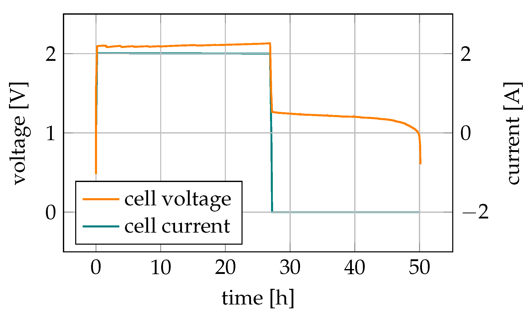
The influence of the SoC is thus an order of magnitude smaller than with traditional technologies. In particular, the temperature and possible aging of the cell and especially of the electrolyte have a stronger effect on the cell voltage than the SoC. It is therefore not possible to determine the SoC from the open-circuit voltage of a zinc–air cell. Figure 4 shows the cell voltage of a zinc–air cell during an active charge and discharge cycle. Both the charging process and the discharging process are performed with a constant current. Even with an active charge current, the change in cell voltage over the charge cycle is so small that neither SoC detection nor effective end-of-charge detection is possible from the cell voltage. In addition, it is problematic that, towards the end of the charging process, an accompanying electrolysis process starts at a similar voltage level, so that overcharging with gassing cannot be detected either. The voltage characteristic during the discharge process is also largely constant. Towards the end of the discharge process, however, there is a voltage drop, therefore deep discharge detection is at least possible with the aid of a conventional voltage threshold. While SoC detection is very difficult this way, the behavior on the other hand has the advantage that applications using a zinc–air cell can be optimized for very constant voltage ranges.

In this article, therefore, it is analyzed whether it is possible to develop a method for detecting the SoC of zinc–air batteries with the help of alternative methods. EIS turned out to be a promising measurement technique to obtain measurement data which depend on the SoC. Due to the special electrode arrangement of the used zinc–air cells, an adapted measurement hardware is presented.

The previous approaches always specified a fixed DC current that was used during measuring the impedance spectra [29,30,31]. This principle can also be applied in practice. However, the current working point must then be left in order to use the working point that was used for training the models. When charging, this can lead to situations where energy generated by a photovoltaic system cannot be utilized at this point in time. When discharging, the energy of the new working point may not be sufficient and additional energy from the grid is needed reach the desired working point. In both cases, there is a monetary loss. This article therefore analyzes whether it is also possible to create a model that generalizes the DC current or the working point. In detail, this means that the models are trained with data from different working points and thus an evaluation with different direct currents is also possible. The acquired measurement data are then combined methods of artificial intelligence to determine the SoC as accurately as possible. Therefore the focus is on a model that generalizes the DC current (=the working point) of the battery during an EIS measurement.

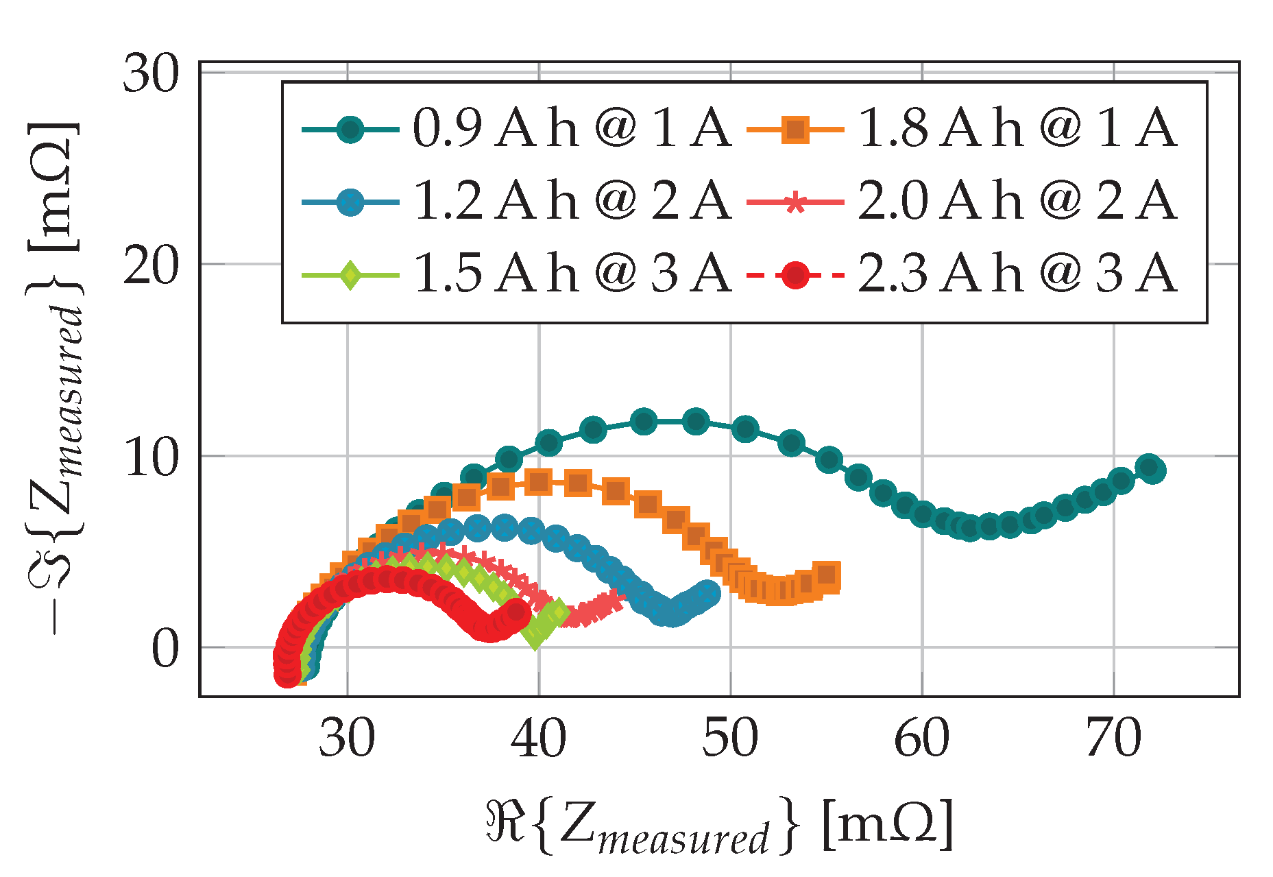
Figure 5 illustrates why this aspect is particularly difficult. The figure shows impedance measurements at different SoC (Ah values) and DC currents (A values). One can see that an increase in the DC current behaves similar to a change in the SoC. Thus, the characteristics are sorted according to their DC currents and not according to the SoC.

3. Setup

EIS determines the impedance, i.e., the AC resistance, of electrochemical systems as a function of the frequency of an AC voltage or current. Electrochemical systems are, for example, batteries. EIS can be used to obtain precious information about the system under investigation and the processes taking place in it. Usually, EIS is performed on batteries by imposing an alternating current, that is, the current of the working electrode is sinusoidally modulated and the resulting voltage and its phase are measured. The DC component of the modulated current is usually set to 0 so that the EIS is charge neutral and the state of charge of the cell is not influenced. Due to the three-electrode technology used in our zinc–air cells, the charge-neutral method cannot be used, as the DC component must be at least as large as the AC amplitude so that there is no switching between charging and discharging during an impedance measurement. The concept of impedance and the complex alternating current theory assume that there is a linear relationship between the amplitudes of voltage and current. In electrochemical systems, this is only the case approximately for small amplitudes, e.g., 1 $\mathrm{m}$$\mathrm{V}$ to 10 $\mathrm{m}$$\mathrm{V}$ [32]. Significantly larger voltage amplitudes, therefore, must not be used for measurement.

In particular, the necessary DC component during an impedance measurement and the three-electrode technology prevent the use of an existing instrument for the measurement of impedance spectra. Therefore, developments for the measurement of impedance spectra of zinc–air, cells as well as adaptations for existing measuring instruments, are presented in this section.

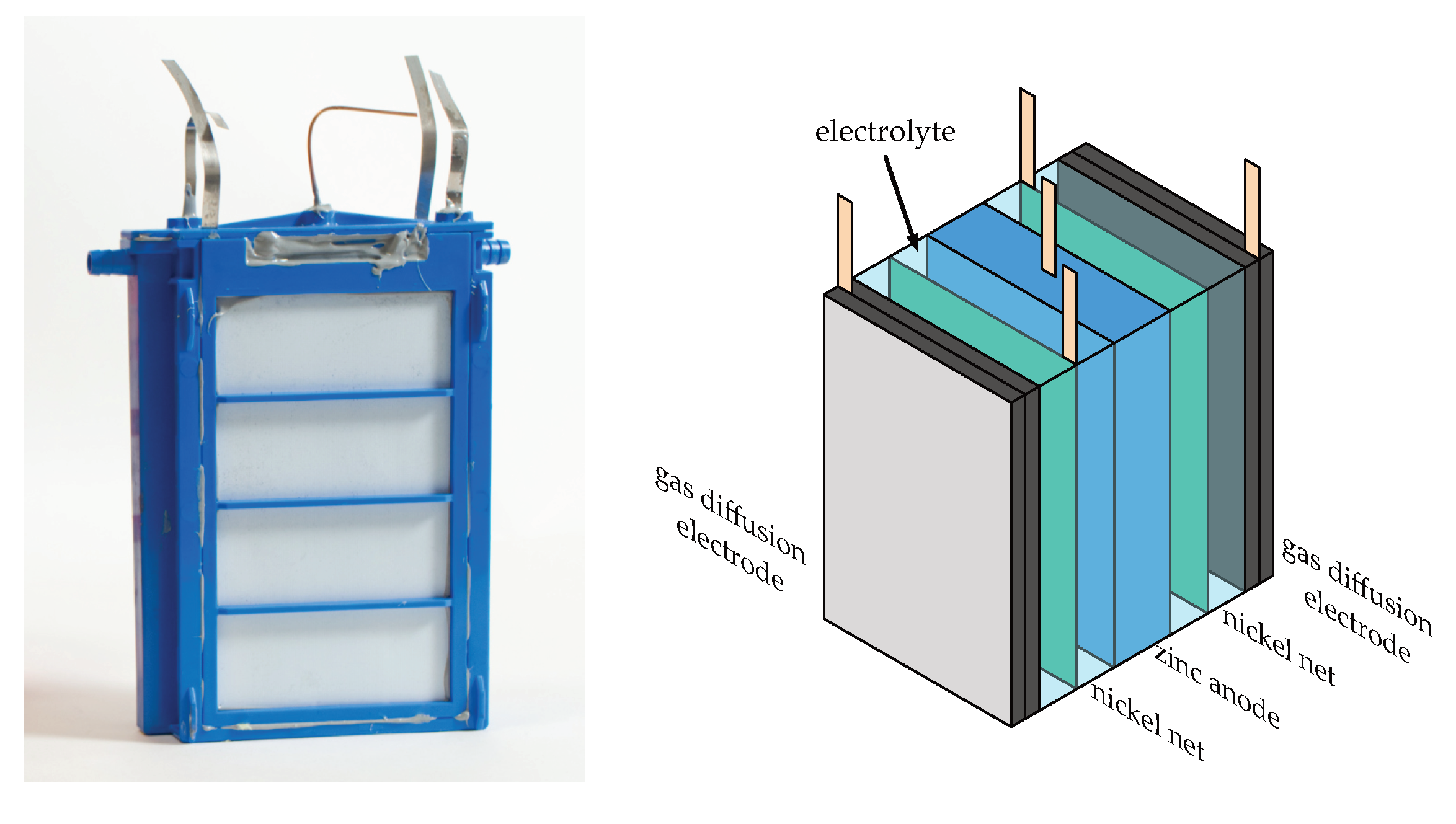
In this article, a rechargeable zinc-air cell from the company 3e Batteriesysteme is used. The cell can be seen in Figure 6 and has a capacity of 100 Ah. Figure 6 also shows the schematic diagram of the internal structure. The cell has a symmetrical structure in order to increase the active surface area. Inside the electrolyte there are nickel nets which serve as positive contacts during the charging process.

The overall structure of the developed circuit is shown in Figure 7. The entire EIS process is controlled by a microcontroller, so that the setup is rather small and field applications are possible. The STM32F4 microcontroller represents the centerpiece of the schematic that controls all of the other peripherals. One of its two digital analog converters is used to output a sine wave at the frequency that is measured. The other digital analog converter creates several constant voltages using a sample and hold circuit that enables the duplication of numbers of outputs as long as constant voltages are being output. These voltages control the amplitude and the offset of the signal. The accuracy of the output signal is kept high, as amplitude and offset are controlled separately. A galvanostatic impedance measurement is preferred, as it is easier to control the current than such a small voltage. Therefore, the output signal is used as input of a current controller that applies the AC current to the battery under test. Last but not least, an external analog digital converter is used to measure both the actual applied AC current and the resulting voltage response of the battery under test. According to MacDonald the amplitude of the voltage response has to remain less than 10 $\mathrm{m}$$\mathrm{V}$ [32]. Therefore, a high precision, high speed analog digital converter, AD7768-4, is used so that the voltage response can be measured with sufficient accuracy despite the voltage offset of the battery. Offset compensation is thus not necessary.

3.1. Signal Generation and Measurement Unit

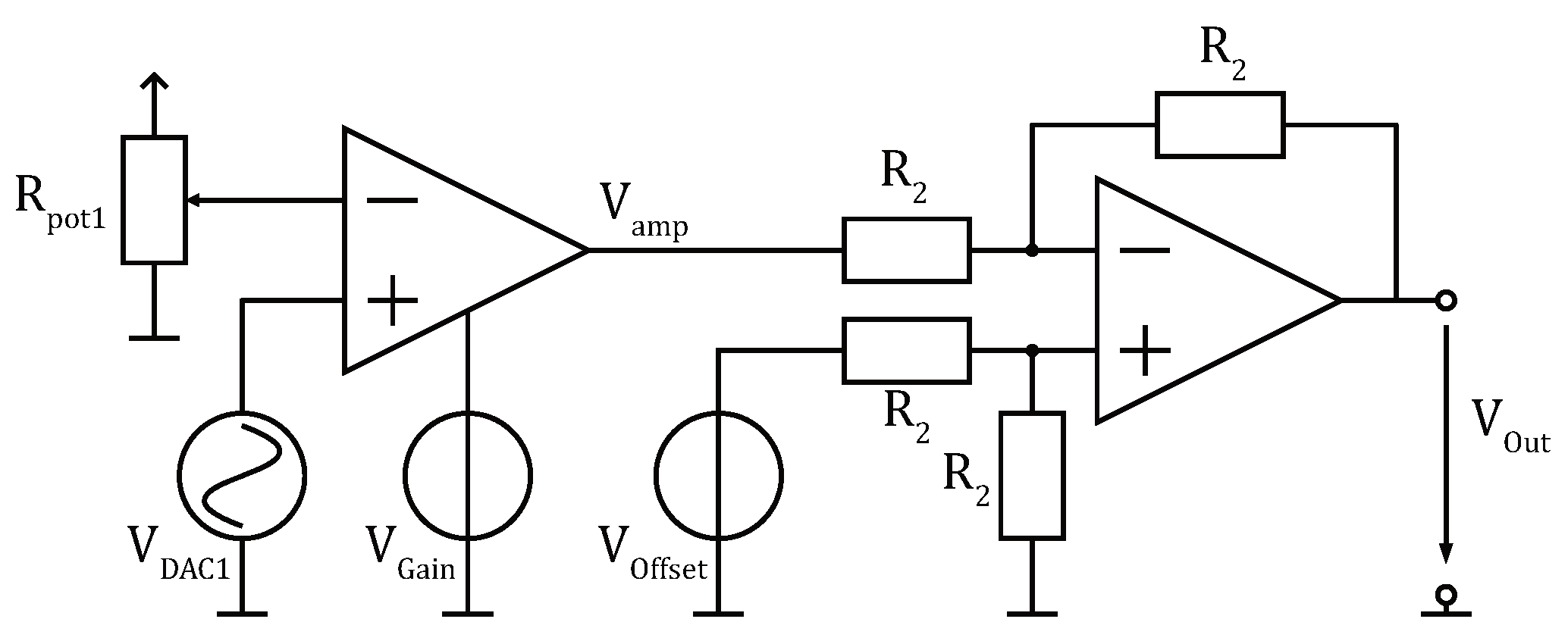
Figure 8 takes a closer look to the signal generation. The sine voltage $V_{DAC1}$ is the digital analog converter output of the microcontroller which oscillates between 0 $\mathrm{V}$ and $3.3$ $\mathrm{V}$. The left amplifier is the voltage controlled gain amplifier LMH6503. It amplifies its differential input voltage. Therefore, $R_{pot1}$ sets the negative input voltage to $1.65$ $\mathrm{V}$ so that the differential input voltage is a symmetrical sine wave. The amplitude of the output signal $V_{amp}$ can be controlled by $V_{Gain}$. The components on the right-hand side implement a difference amplifier. As all resistors that belong to this circuit have an equal resistance,

$$V_{out}=V_{offset}-V_{amp}$$

applies to the output voltage. Accordingly, voltage $V_{amp}$ is inverted and shifted by an offset. As $V_{amp}$ is a symmetrical sine wave, and only the phase difference between the applied current and the voltage response is evaluated for determining the impedance, an inversion of $V_{amp}$ does not have any impact on the measurement.

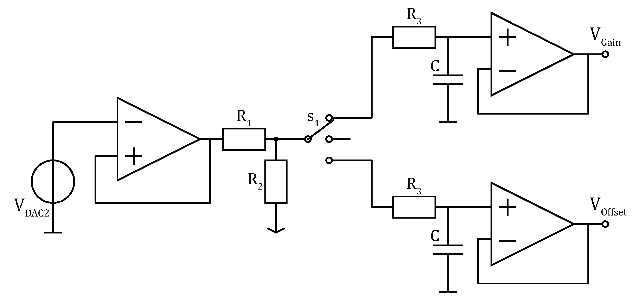
$V_{Gain}$ and $V_{Offset}$ are generated by a single digital analog converter output using a sample and hold circuit shown in Figure 9. The first amplifier implements a voltage buffer that decreases the current of the digital analog converter. The following voltage divider shifts the digital analog converter output range to symmetrical ±1 V range by referencing the lower pin of $R_2$ to a negative voltage. Thereby, the offset voltage of $V_{out}$ can correspond to either a constant charging or a constant discharging current. The actual sampling is implemented by a digitally controlled analog switch $S_1$ while the capacitors hold the sampled voltages. The circuit is controlled by the microcontroller that uses a timer with three output compare channels that cyclically generate interruptions at three different time points. During the first interruption, the switch is set to middle position that is not connected. The second interruption changes the output of the digital analog converter output voltage to the value of the next clamp. Finally, the switch is switched to this clamp charging the corresponding capacitor. The final voltage buffers output the voltage that is stored in the capacity. As the input current of an operational amplifier is rather small, the voltage of the capacity is almost constant, even when the digital analog converter signal is removed when switching to the other path.

3.2. Current Controller

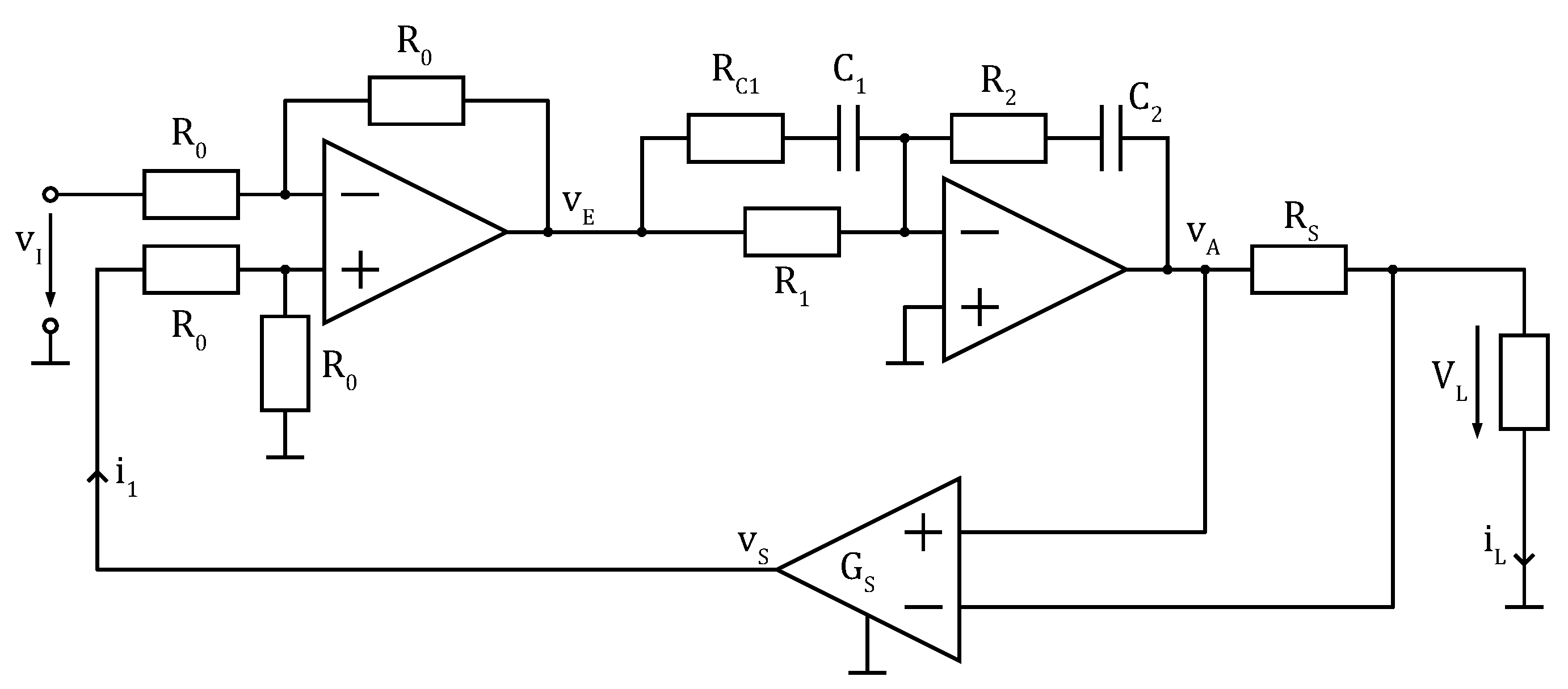
Regarding the control of the current, the first question that arises here is whether digital or analog control is better. Although it is much easier to adapt the controller parameters to the system being measured, the time constants are very small, so that the sampling intervals of a digital control would lead to instabilities. Therefore, an analog control system that is based on operational amplifier is used. The OPA549 is used as the output operational amplifier, which can directly drive the required currents. A possible implementation using an instrumental amplifier to measure the load current $i_L$ and two operational amplifier that implement a differential amplifier and a PID controller is shown in Figure 10. The main purpose of the instrumentation amplifier is to measure and amplify the differential voltage of the shunt resistor $R_S$ and to reference its output voltage

$$v_S\left(t\right)=\left(v_A\left(t\right)-v_L\right)·G_S=R_S{i}_L\left(t\right)·G_S$$

(6)

to ground potential. The value $v_I\left(t\right)$ sets the desired load current multiplied by $R_S$ and $G_S$:

$$v_I\left(t\right)=i_{L,desired}·R_S·G_S.$$

(7)

Therefore, the operational amplifier on the left-hand side implements the differential amplifier with a gain of 1 and determines the negative of the measured error $e\left(t\right)$:

$$v_E\left(t\right)=v_S\left(t\right)-v_I\left(t\right)=-e\left(t\right).$$

(8)

The actual controller is implemented by the op amp on the right-hand side. As an approximation, the inputs of an operational amplifier can be regarded as current-less, so that the current flowing through $R_2$ and $C_2$ can be assumed to equal $i_1\left(t\right)$. Therefore, $i_{11}$ and $i_{12}$ form two components of the regulating variable:

$$i_2\left(t\right)=i_1\left(t\right)=i_{11}\left(t\right)+i_{12}\left(t\right)$$

(9)

Due to the negative feedback, both input terminals of the operational amplifier are forced to ground potential. Therefore, the current $i_{11}\left(t\right)$ can be calculated by

$$i_{11}\left(t\right)=\frac{1}{R_1}{v}_E\left(t\right)=-\frac{1}{R_1}e\left(t\right).$$

(10)

Furthermore, $i_{12}$ is defined by

$$i_{12}\left(t\right)=C_1\frac{d{v}_E\left(t\right)}{dt}=-C_1\frac{de\left(t\right)}{dt}.$$

(11)

The output voltage $v_A$ is determined by the current $i_2:$

$$\begin{array}{cc}\hfill v_A\left(t\right)& =-i_2{R}_2-\frac{1}{C_2}\int i_2\left(t\right)dt.\end{array}$$

(12)

Inserting Equations (9) to (11) results in

$$v_A\left(t\right)=-\frac{R_2}{R_1}{v}_E\left(t\right)-\frac{1}{R_1{C}_2}\int v_E\left(t\right)dt-R_2{C}_1\frac{d{v}_E\left(t\right)}{dt}-\frac{C_1}{C_2}{v}_E\left(t\right),$$

(13)

$$v_A\left(t\right)=-\left(\frac{R_2{C}_2+R_1{C}_1}{R_1{C}_2}\right)v_E\left(t\right)-\frac{1}{R_1{C}_2}\int v_E\left(t\right)dt-R_2{C}_1\frac{d{v}_E\left(t\right)}{dt},$$

(14)

$$v_A\left(t\right)=\left(\frac{R_2}{R_1}+\frac{C_1}{C_2}\right)e\left(t\right)+\frac{1}{R_1{C}_2}\int e\left(t\right)dt+R_2{C}_1\frac{de\left(t\right)}{dt}.$$

(15)

Comparing the last equation with the equation of a PID controller

$$y\left(t\right)=K_p·e\left(t\right)+K_i\int e\left(\tau \right)d\tau +K_d\frac{de\left(t\right)}{dt}$$

(16)

results in the following parameters:

$$K_p=\frac{R_2}{R_1}+\frac{C_1}{C_2},$$

(17)

$$K_i=\frac{1}{R_1{C}_2},$$

(18)

$$K_d=R_2{C}_1.$$

(19)

In the next step the controller parameters were optimized. As the load $R_L$ represents the battery under test, which cannot be described sufficiently accurately by a resistor, an equivalent circuit consisting of a voltage source, a series resistor and a RC parallel circuit was used as $R_L$. The circuit simulator Microcap already includes an optimizer. During the optimization the controller parameters were tuned to minimize the expression RMS(v(VE)) when a step function is applied to the input. Thus, the root mean square of the voltage $V_e$, which in turn represents the control deviation should be as small as possible. The optimized circuit was then produced on a printed circuit board. Care must be taken to ensure that the connections that drive the high current to the battery under test are sufficiently sized.

First, the step response of the current controller was measured using a test impedance, whereby the target signal was generated with the aid of a function generator. The voltage $V_S$ is used to measure the current and shown in Figure 11. The step response of the current controller asymptotically follows the input signal without overshoot and thus demonstrates the behavior of a first order low pass filter. The test signal transitions to 500 $\mathrm{m}$$\mathrm{V}$, so that the time constant can be read when 315 $\mathrm{m}$$\mathrm{V}$ is reached. This occurs after 43 μ$\mathrm{s}$ and thus corresponds to a cutoff frequency of 23 $\mathrm{k}$$\mathrm{Hz}$. The current regulator is thus sufficiently fast for frequencies usually measured during EIS.

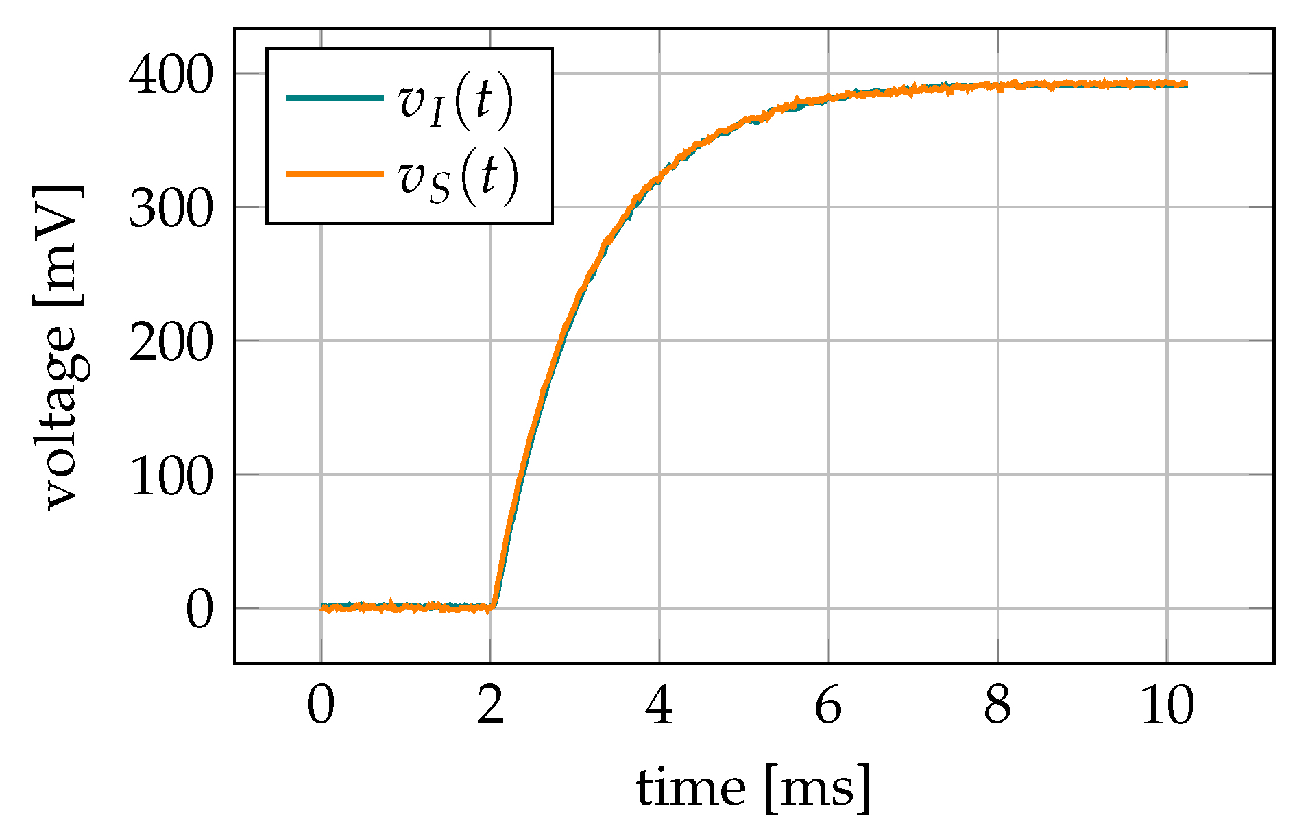
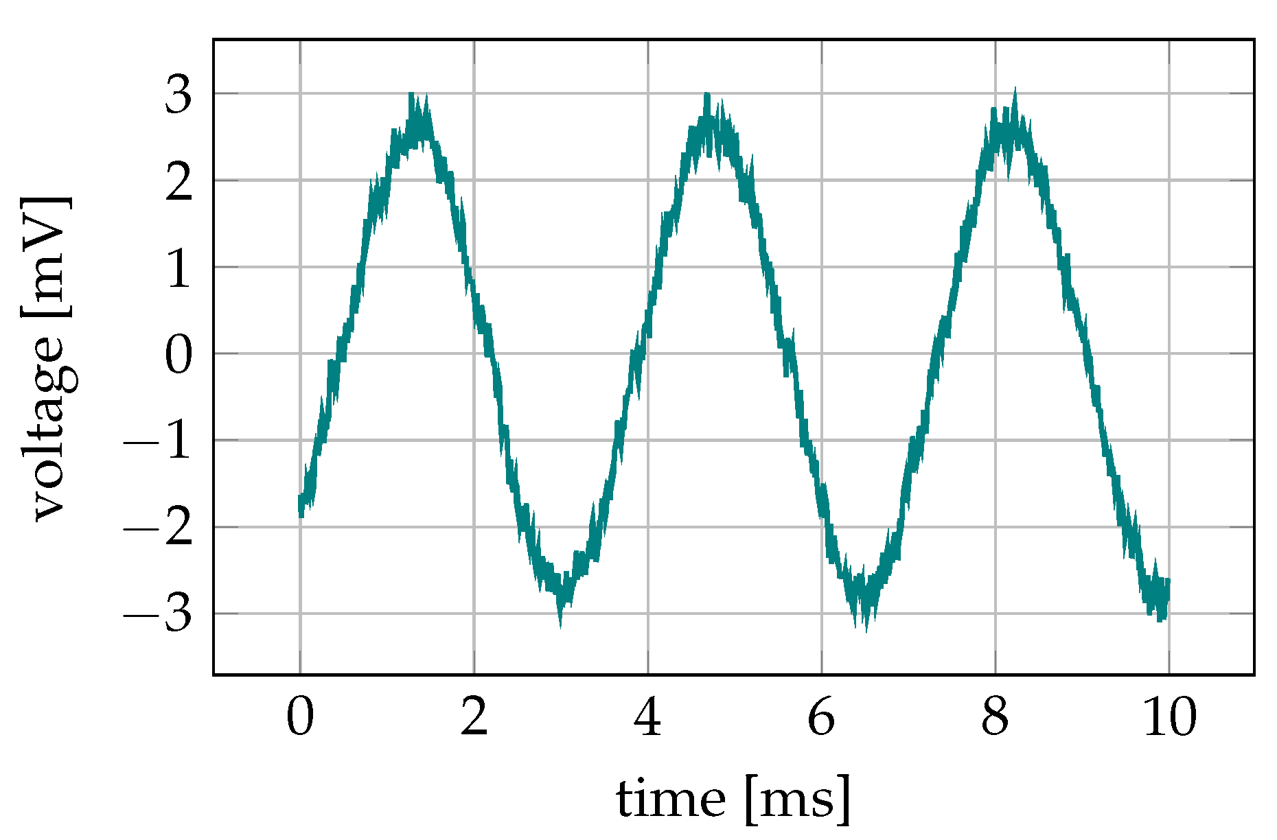
Figure 12 and Figure 13 show the results when combining the signal generation unit and the current controller. Once again, the test impedance was used as $R_L$, which was designed on the basis of Kiel’s dissertation [33]. First of all, it is noticeable that there is no visible difference between these two signals. However, the signals correspond rather to a first order delay element than a step function. This is due to the fact that the input signal is generated by the signal generation. The charging of the capacitor in the sample and hold part is mainly responsible for the slow voltage rise. Therefore, the current controller is dimensioned sufficiently fast to output the generated signals.

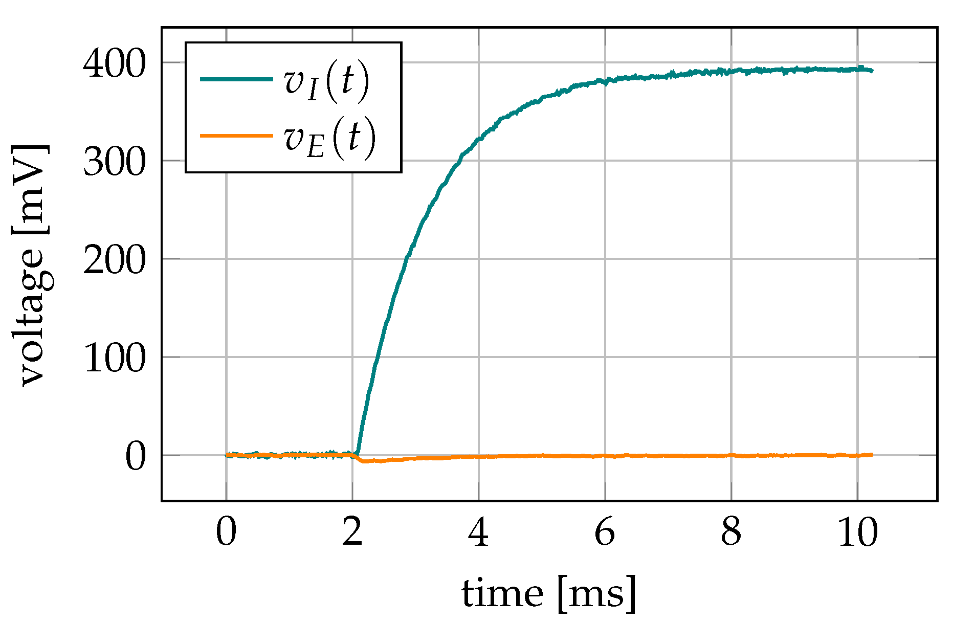
Figure 13 takes a closer look at the control deviation $V_E$. At the beginning of the step, when the slope is at its maximum, there is a small control deviation. In relation to the step height of 400 $\mathrm{m}$$\mathrm{V}$, the maximum deviation of $6.3$ $\mathrm{m}$$\mathrm{V}$ is still relatively small.

3.3. Drift Compensation

Due to the three-electrode technology, the measurement of the impedance spectra can only be performed during a charging process and during a discharging process, respectively, so that the state of charge of the cell changes to a certain extent during the measurement. As the measurement time at low frequencies is up to 30 $\mathrm{s}$, the DC component of the voltage measurement may change during the measurement. The voltage change is particularly large at the beginning of charging or discharging processes as the slowest processes have yet to decay. 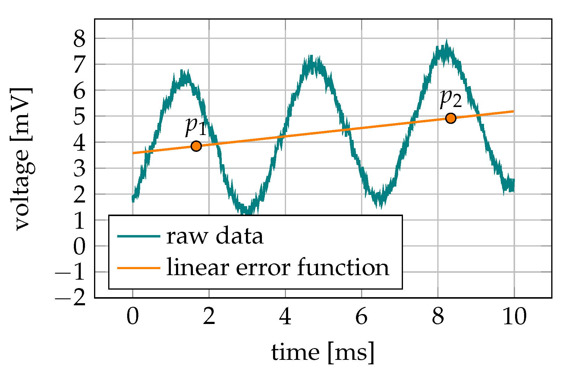The voltage signal of such a case is shown in Figure 14 as an example.

The resulting error is minimized by modeling the DC voltage component in a linear way and subtracting it from the characteristic of the voltage. Linear functions are determined by two points. Thus, the mean values of the first sine period ($p_1$) and the last sine period ($p_2$) of the voltage signal are being determined. The mean value of a sine period without offset is zero. Therefore, for the evaluated periods, the mean value can be used to determine the offset value $p_{i,v}$. The associated time component $p_{i,t}$ of the points corresponds to the midpoint of each period. Thus, the point ($p_1$) of the first period is given by its components

$$p_{i,v}=\sum _{s=0}^{s_p}\frac{v_s}{s_p},$$

(20)

$$p_{i,t}=\sum _{s=0}^{s_p}\frac{t_s}{s_p}=\frac{1}{2·f}.$$

(21)

Here, s implements a control variable that passes through the voltage samples $v_s$ and their corresponding time points $t_s$. The number of values corresponding to the period is given by $s_p$ and the measured frequency by $f_k$. The equation of a line described by $p_1$ and $p_2$ is then subtracted from the raw measurement data. As can be seen in Figure 15, the error is almost completely eliminated.

3.4. Measurement Data

Afterwards, the corrected voltage signal and the measured current signal are Fourier transformed to $\underline{V}$ and $\underline{I}$. As only one frequency is applied at a time, only this frequency has to be evaluated. To save computational effort, the Goertzel algorithm can therefore be used [34]. Finally, the impedance $\underline{Z}$ of frequency k is calculated by

$${\underline{Z}}_k=\frac{{\underline{V}}_k}{{\underline{I}}_k}.$$

(22)

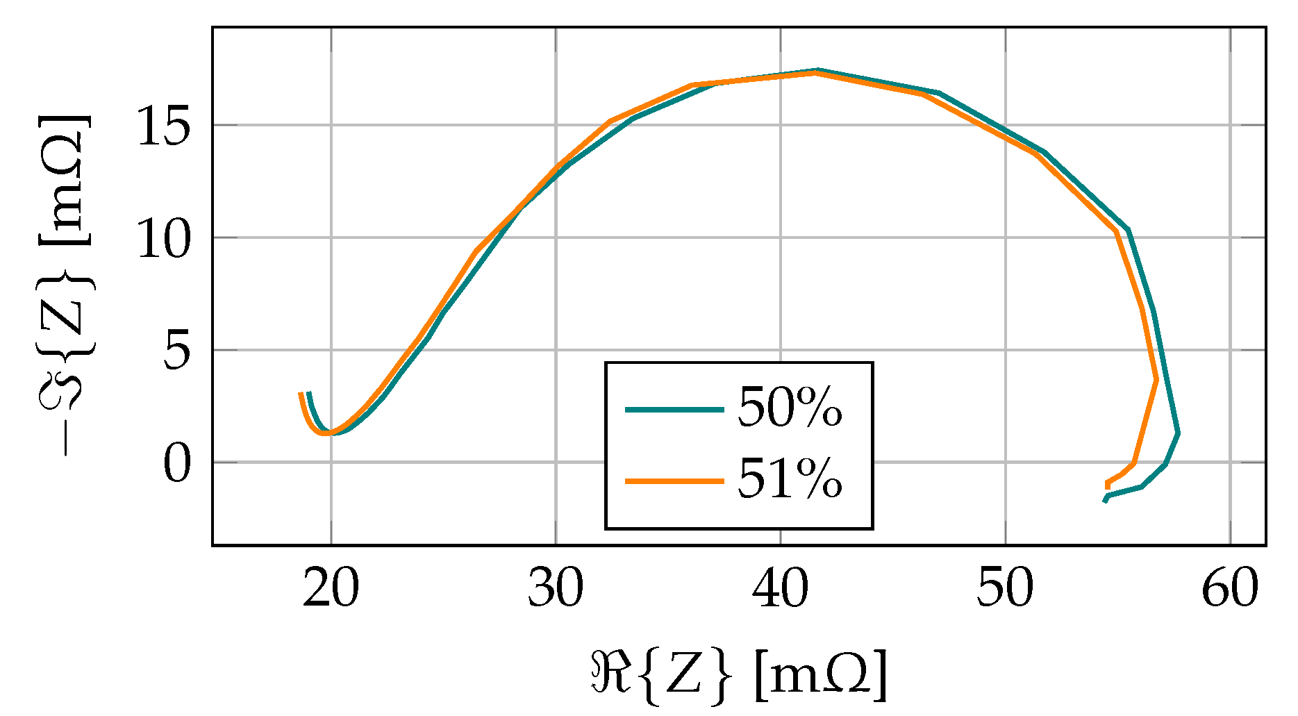
Several impedances for different frequencies are measured quickly one after the other and can be combined to a spectrum. Figure 16 shows some example measured spectra data. Between the measurements, the cell was discharged for 45 min, therefore the spectra are not exactly identical. It can already be seen here that especially the low-frequency components, which are found on the right-hand side, are influenced by the state of charge.

3.5. Adapter Board

Another possibility for measuring impedance spectra is the use of a commercial impedance spectroscope. The most difficult challenge in the search for a suitable product is the simultaneous application of a DC current during the impedance measurement. This is essential for the developed zinc–air cell, as it uses a three-electrode technology and the respective charge or discharge region must not be left during the impedance measurement. If no DC current is applied, the cell would be charged during the first half-period of the sine wave and discharged during the second half-period. The EISmeter from the Digatron company was finally chosen.

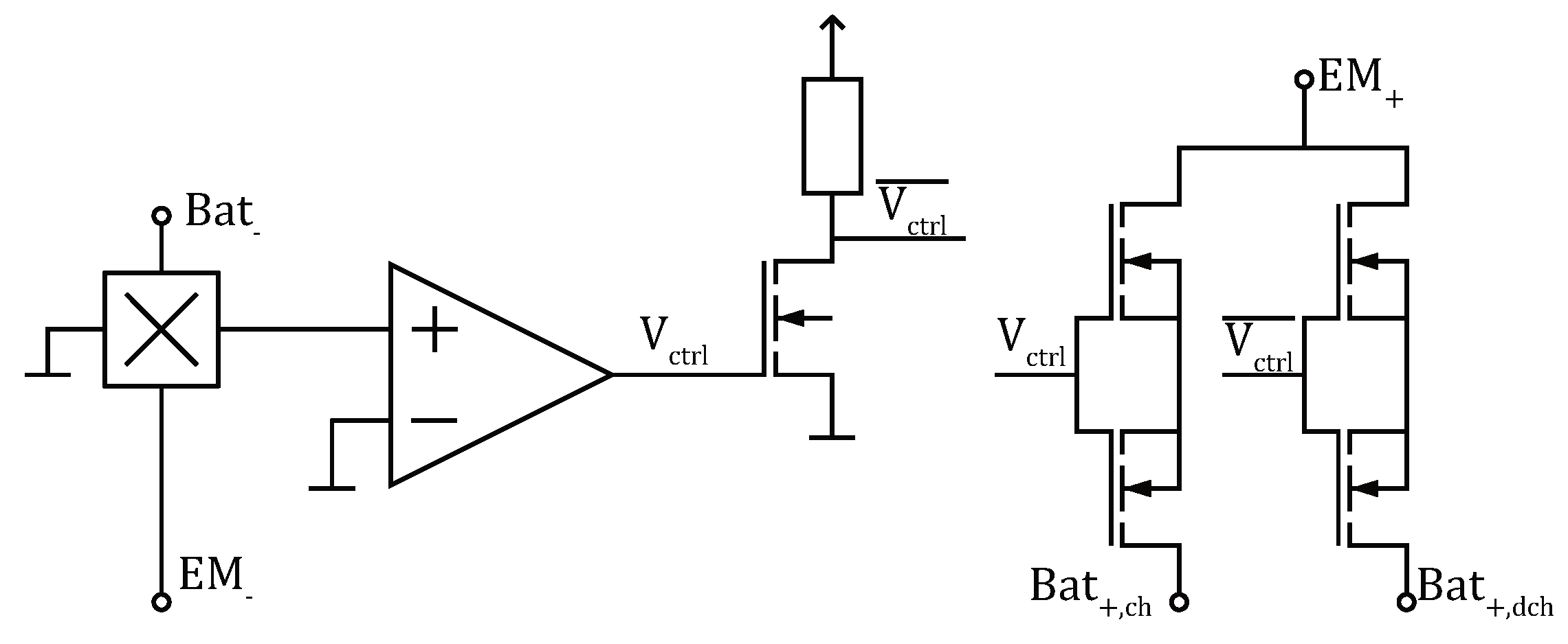
Although the EISmeter can apply a DC current during the measurement, it is only designed for two-pole cells. Besides the manual reconnection, one way to still use zinc–air cells with three-electrode technology is to use two channels of the EISmeter for one cell. One channel is taken exclusively during charging of the cell and is connected to the charging electrode and one channel is connected to the air cathode is used only during discharging of the cell. Of course, the method has the disadvantage that it reduces the number of simultaneous tests by half. To overcome this, an electrode changer board was developed. The corresponding circuit is shown in Figure 17. It is based on a Hall-effect current sensor from Allegro Microsystems. An operational amplifier, which works as a comparator, detects the direction of the current, i.e. whether the cell is being discharged or charged. Depending on the case, a different current path is enabled to the appropriate electrode. An identical control is also available for the path of the voltage measurement, whereby smaller transistors are used here.

4. Data Generation

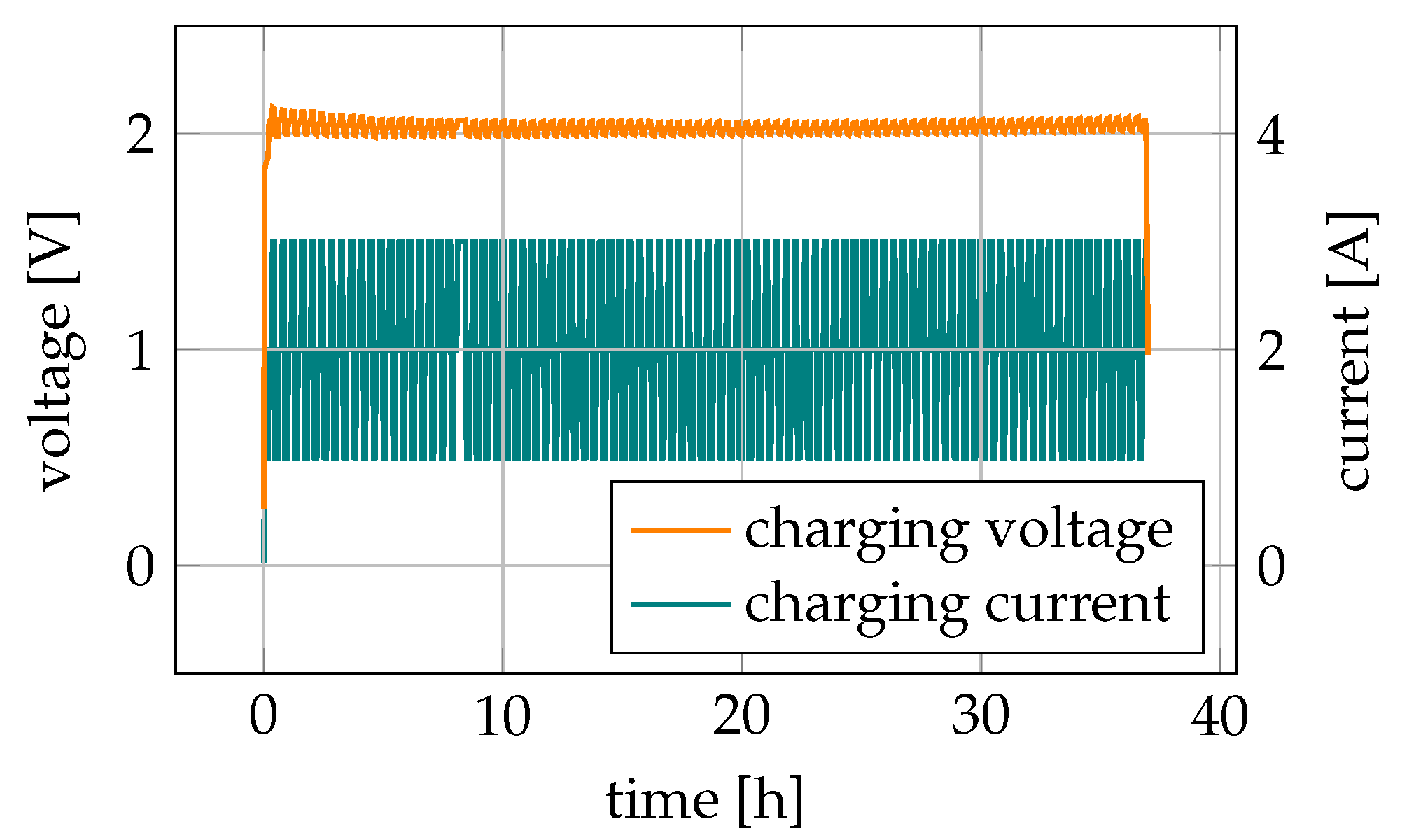
To generate measurement data, a procedure shown in Figure 18 and Figure 19 is used. Here, zinc–air cells are continuously charged or discharged with an alternating current of 1 $\mathrm{A}$, 2 $\mathrm{A}$, or 3 $\mathrm{A}$. This means that the charging process starts with 1 $\mathrm{A}$. A short delay is made until the cell voltage has become familiar with the current and a measurement of the impedance spectrum is started. After that, the charging current is increased to 2 $\mathrm{A}$; again a short delay is made and the next impedance measurement is started. The same is performed for 3 $\mathrm{A}$ and then it starts again at 1 $\mathrm{A}$. As expected, this also results in a change in the battery voltage.

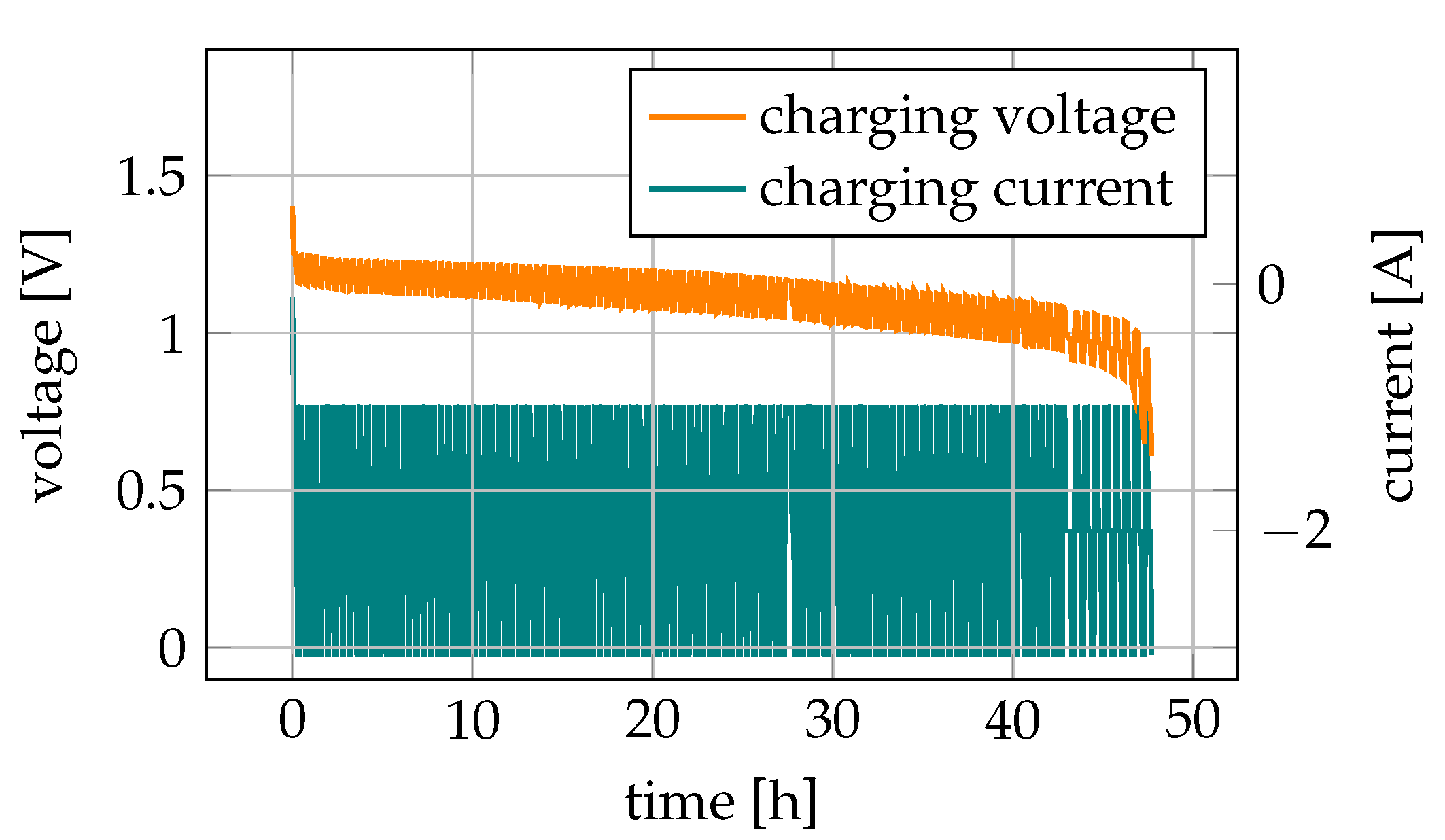
Meanwhile, the applied charge is counted so that, in this scenario without any breaks, the actual state of charge is known and can be used as target values for supervised learning. Once the cell is full, the discharge process starts using the identical technique. Therefore, discharging processes have been recorded where the discharge current was regularly alternated between 1 $\mathrm{A}$, 2 $\mathrm{A}$, and 3 $\mathrm{A}$. The resulting voltage curve and the corresponding discharge current for one discharge cycle are shown in Figure 19.

After several charge and discharge cycles, there is no random division of the resulting data into training data and test data, but the measurements at 1 $\mathrm{A}$ and 3 $\mathrm{A}$ form the training data set and the measurements at 2 $\mathrm{A}$ form the test data set. This ensures that the results correspond to an actual generalization of the working point. The hyperparameters are optimized by cross-validating the training set only to prevent data leakage. Of course, the feature vector must be extended to include the DC current value, so that the following feature vector is now obtained:

$$\begin{array}{c}{x}_i=[I_{\mathrm{bat},\mathrm{DC}},\Re \left\{Z_{i,1}\right\},\dots ,\Re \left\{Z_{i,m}\right\},\Im \left\{Z_{i,1}\right\},\dots ,\Im \left\{Z_{i,m}\right\},\\ \hspace{1em}\hspace{1em}\hspace{1em}\hspace{1em}\hspace{1em}\hspace{1em}\hspace{1em}\hspace{1em}\hspace{1em}\hspace{1em}\hspace{1em}\hspace{1em}\hspace{1em}\hspace{1em}\hspace{1em}\hspace{1em}|Z_{i,1}|,\dots ,|Z_{i,m}|,\varphi \left(Z_{i,1}\right),\cdots ,\varphi \left(Z_{i,m}\right)].\end{array}$$

(23)

5. Methods

Typically, the measured impedance spectra are used to parameterize an electrochemical equivalent circuit of the Battery Under Test. In the context of generalizing the DC current during impedance measurement, machine learning techniques are alternatively used. In the context of this paper, artificial neural networks and support vector regression are used for this purpose. These methods are briefly described in this section.

5.1. Artificial Neural Networks

ANN are networks of artificial neurons, each of them inspired by the biological model. McCulloch and Pitts introduced a threshold element as first artificial neuron that outputs a Boolean value $o_j$ depending on the sum of input signals $x_i$ [35]. By now, a commonly used implementation of a neuron is the perceptron model, which extends the threshold element by a weighting of the input signals $w_{ij}$ [36]:

$$o_j=\left\{\begin{array}{ll}1& \sum _i{w}_{ij}{x}_i+b>0\\ 0& \mathrm{otherwise}\end{array}\right.$$

(24)

The general structure of feed forward networks is shown in Figure 20 and allows only a signal flow in forward direction. There are also network structures that allow a feedback to a previous layer, e.g., Recurrent Neural Networks. Several neurons are organized in layers. When using perceptron neurons, these networks are called Multilayer Perceptron. The first layer is called the input layer and represents the features of an input sample extended by a constant bias. The bias can be used as a threshold value by the following layer. Here, only one hidden layer is illustrated, but multiple hidden layers are also possible. The signal flows through all hidden layers until it reaches the output layer. Each neuron in the output layer represents an output value [37].

Multilayer perceptron networks are used in applications where an input sample is associated with an output class or an output variable. The input example can thereby be described in a higher-dimensional feature space. The structure is characterized in particular by the fact that the order in which example data are evaluated by the previously trained network has no influence on the individual result, the network has no memory.

In contrast, a Recurrent Neural Network, for example with an Elman structure, stores values of the hidden units within the feedback loop. The values are then available as input values in the subsequent data set. The output of the network thus also depends on the internal state of the network, which is determined by the previous data. Recurrent Neural Networks are therefore very well suited for modeling sequences, as found in time series analysis. They are also successfully used for the analysis of sentences, which consist of words and letters.

Training Algorithms

Training algorithms are used to set weights of each neuron. When small logic functions (AND, OR, etc.) are patterned, it is possible to manually set those weights. However, ANNs are frequently used in applications with huge datasets. Therefore, algorithms have been developed that autonomously optimize the weights of the network. These algorithms can be divided into supervised and reinforced learning. In this thesis, supervised learning is used exclusively, which means that the training samples also contain target values $t_j$ for the output j.

One example is the Perceptron Learning Rule that works for binary input and output signals. The idea is that the weight is incremented when the output is 0, but should be 1; the weight is decremented when the output is 1, but should be 0; and the weight left unchanged, when the output corresponds to the expectation [36]:

$$\begin{array}{c}\Delta w_{ij}^{perceptron}=\alpha ·\left(t_j-o_j\right)·x_i\\ \\ w_{ij}(k+1)=w_{ij}\left(k\right)+\Delta w_{ij}\end{array}.$$

(25)

where $t_j$ is the target value and $\alpha$ sets the learning rate. However, this approach only works when all training data is linear separable.

The delta rule overcomes this problem by minimizing the error function

$$E_{\Delta }=\sum _j\frac{1}{2}{\left(t_j-o_j\right)}^2$$

(26)

using a gradient decent. This means that the activation function has to be derivable. The weight space of the neurons is moved against the direction of the gradient of $E_{\Delta }$ with respect to each weight

$$\frac{\partial E_{\Delta }}{\partial w_{ij}}=\frac{\partial \frac{1}{2}{\left(t_j-o_j\right)}^2}{\partial w_{ij}}.$$

(27)

As we differentiate with respect to the weights of jth neuron, the weights of the other neurons in the sum vanishes. Inserting

$$o_j=\varphi \left(\sum _i{w}_{ij}{x}_i\right)=\varphi \left(v\right)$$

(28)

and applying the chain rule results in

$$\frac{\partial E_{\Delta }}{\partial w_{ij}}=-\left(t_j-o_j\right)·x_i·{\varphi }^{\prime }\left(v\right).$$

(29)

Once again, a learning rate is used for weight update and the minus sign is eliminated for moving in the direction of the minimum. This results in the updated equation

$$\Delta w_{ij}^{delta}=\alpha \left(t_j-o_j\right)·x_i·{\varphi }^{\prime }\left(v\right).$$

(30)

The delta rule is only applicable to single layer–layer neural networks. A generalized form is the Error Backpropagation learning. It uses the very same error function to minimize:

$$E_{ebp}=\sum _j\frac{1}{2}{\left(t_j-o_j\right)}^2.$$

(31)

However, the adjustment of the weights depends on whether the neuron is in the output layer or in the hidden layer:

$$\Delta w_{ij}^{ebp}=-\alpha \frac{\partial E}{\partial w_{ij}}=\alpha {\delta }_j{o}_i$$

(32)

and

$${\delta }_j=\left\{\begin{array}{ll}{\varphi }^{\prime }\left(v\right)\left(t_j-o_j\right)& \mathrm{if}j\mathrm{corresponds}\mathrm{to}\mathrm{an}\mathrm{output}\mathrm{neuron}\\ {\varphi }^{\prime }\left(v\right)\sum _k{\delta }_k{w}_{jk}& \mathrm{if}j\mathrm{corresponds}\mathrm{to}\mathrm{hidden}\mathrm{neuron}\end{array}\right..$$

(33)

Here, i corresponds to prior neurons of j and k corresponds to subsequent neurons. This means that $o_i$ is the input of neuron j, for the first layer $o_i$ equals $x_i$. Moreover, for hidden neurons the weight adjustment depends on the error of the subsequent neurons. Thus, the error is back propagated to hidden neurons. The Error Backpropagation algorithm is also a gradient decent based, which makes it vulnerable for finding local minima. Therefore, different solutions are possible for different weight initialization.

Secondly, the algorithm tends to oscillate when the learning rate is too large. Several approaches make use of a momentum term in order to smooth the solution process. The tendency for oscillations can also be tackled by lowering the learning rate constant. However, this also decreases the training speed. In contrast, the directional search extension can speed up the solution process. The idea is to look for a minimum in gradient direction before the calculation for a new gradient. The minimum in gradient direction can be found using the Newton–Raphson method.

In Recurrent Neural Networks, the Error Backpropagation algorithm cannot be used in its original form due to the recurrent loops preventing it. With the help of the Backpropagation Through Time method, this problem can be overcome. Backpropagation Through Time is a method based on Backpropagation. Here, the Error Backpropagation method is extended by a time factor. As the output of a Recurrent Neural Network depends on the order of the data, the training data are an ordered sequence of k input and output pairs $\langle x_1,y_1\rangle ,\langle x_2,y_2\rangle ,\dots ,\langle x_k,y_k\rangle$. In order to subsequently apply the original Backpropagation algorithm, the Recurrent Neural Network must be unfolded. The unfolded network thus contains k inputs. The recurrent components of the original network are completely duplicated for each required time step. The Backpropagation algorithm is then applied to the expanded network.

The complexity of the resulting unfolded network increases drastically when increasing the length of the training sequence. This can lead to problems when using the Backpropagation algorithm as, as shown in the corresponding Equation (33), the variations of the weights also depend on the gradients of the errors of the subsequent neurons. In case of a long sequence, the error term of the unfolded network is multiplied accordingly many times. Provided that the error term is smaller than 1, a frequently repeated multiplication results in a value close to 0 (vanishing gradient problem). On the other hand, the magnitude of the error term could also be larger than 1, so that after repeated multiplication the resulting gradients explode and the gradient descent becomes unstable. For deep recurrent neural networks the Backpropagation Through Time Algorithm is therefore not suitable, instead other structures such as the Long Short-Term Memory module should be used.

5.2. Support Vector Regression

The basic idea of $ϵ$-SVR is finding the flattest function $f\left(x\right)$ whose deviation from the training data is not larger than a given parameter $ϵ$. In case of a linear function

$$f\left(x\right)=\langle w,x\rangle +b$$

(34)

where $\langle ·,·\rangle$ denotes the dot product, the resulting optimization problem is given by:

$$\begin{array}{ll}\mathrm{minimize}& \frac{1}{2}{\Vert w\Vert }^2\\ \\ \mathrm{subject}\mathrm{to}& \begin{array}{c}\left\{\begin{array}{ccc}{y}_i-\langle w,x_i\rangle -b& \le & ϵ\\ \langle w,x_i\rangle +b-y_i& \le & ϵ\end{array}\right\}\end{array}\end{array}$$

(35)

Here, the flatness is defined as norm of the parameter vector, ‖w${\Vert }^2=\langle w,w\rangle$. The constraints mean, that training data with an error smaller than $ϵ$ is not taken into account while errors larger than $ϵ$ are not acceptable [38,39].

However, depending on the type of function, it is not always feasible to find a function that keeps the deviation small enough for all training data. Under certain circumstances, this function does not exist. Therefore, the margin can be softened depending on the training data by using slack variables ${\xi }_i$ and ${\xi }_i^{*}$ which belong to a positive or negative error, respectively:

$$\begin{array}{ll}\mathrm{minimize}& \frac{1}{2}{\Vert w\Vert }^2+C\sum _{i=1}^{\iota }\left({\xi }_i+{\xi }_i^{*}\right)\\ \\ \mathrm{subject}\mathrm{to}& \begin{array}{c}\left\{\begin{array}{ccc}{y}_i-\langle w,x_i\rangle -b& \le & ϵ+{\xi }_i\\ \langle w,x_i\rangle +b-y_i& \le & ϵ+{\xi }_i^{*}\\ {\xi }_i,{\xi }_i^{*}& \ge & 0\end{array}\right\}\end{array}\end{array}$$

(36)

The margin is extended by the slack variables, so that deviations larger than $ϵ$ are now acceptable, but penalized. Figure 21 illustrates the development of the penalty. As long as the deviation is within the $ϵ$ margin, no penalty is applied. If the deviation becomes larger than $ϵ$, the penalty increases with a slope defined by the parameter C.

Thus, there is a trade-off between the flatness of the resulting function and the size of the remaining deviation that can be set by constant C. This trade-off is especially important, as flatter functions tend to be more robust to unseen data.

Lagrange multipliers can be used to find the extremum of a (optimization) function $f\left(x\right)$ with constraints $g\left(x\right)$. Essentially, at the point of extremum, the gradients of $f\left(x\right)$ and $g\left(x\right)$ need to point in the same direction. Otherwise, it would be possible to increase or decrease the value of $f\left(x\right)$ by moving along $g\left(x\right)$. However, while the gradient vectors have to point in the same direction, they do not necessarily have the same length. Therefore, the Lagrange multiplier $\lambda$ is added to the gradient of $g\left(x\right)$ in order to re-scale its vector length. The resulting constraint for an extremum of $f\left(x\right)$ at $g\left(x\right)$ is

$$\nabla f\left(x\right)=\lambda \nabla g\left(x\right).$$

(37)

Applied to Equation (36) $f\left(x\right)-\lambda g\left(x\right)$ gives the so-called Lagrangian:

$$\begin{array}{l}L:=\frac{1}{2}{\Vert w\Vert }^2+C{\displaystyle \sum _{i=1}^{\iota }}\left({\xi }_i+{\xi }_i^{*}\right)-{\displaystyle \sum _{i=1}^{\iota }}\left({\eta }_i{\xi }_i+{\eta }_i^{*}{\xi }_i^{*}\right)+\\ \hspace{1em}\hspace{1em}\hspace{1em}\hspace{1em}-{\displaystyle \sum _{i=1}^{\iota }}{\alpha }_i\left(ϵ+{\xi }_i-y_i+\langle w,x_i\rangle +b\right)+-{\displaystyle \sum _{i=1}^{\iota }}{\alpha }_i^{*}\left(ϵ+{\xi }_i^{*}+y_i-\langle w,x_i\rangle -b\right)\end{array}$$

(38)

where ${\eta }_i$, ${\eta }_i^{*}$, ${\alpha }_i$, and ${\alpha }_i^{*}$ represent the Lagrange multipliers. According to the saddle point condition of Equation (37), the partial derivatives of L with respect to $\omega$, b, ${\xi }_i$, and ${\xi }_i^{*}$ have to be zero:

$$\frac{\partial L}{\partial b}=\sum _{i=1}^{\iota }\left({\alpha }_i^{*}-{\alpha }_i\right)=0$$

(39)

$$\frac{\partial L}{\partial \omega }=\omega -\sum _{i=1}^{\iota }\left({\alpha }_i-{\alpha }_i^{*}\right)x_i=0$$

(40)

$$\frac{\partial L}{\partial {\xi }_i}=C-{\alpha }_i-{\eta }_i=0$$

(41)

$$\frac{\partial L}{\partial {\xi }_i^{*}}=C-{\alpha }_i^{*}-{\eta }_i^{*}=0$$

(42)

Constants ${\alpha }_i$ and ${\alpha }_i^{*}$ define the resulting support vectors. ${\eta }_i$ and ${\eta }_i^{*}$ can be eliminated through Equations (41) and (42) as ${\eta }_i^{\left(*\right)}=C-{\alpha }_i^{\left(*\right)}$. Furthermore, $\omega$ can also be expressed as

$$\omega =\sum _{i=1}^{\iota }\left({\alpha }_i-{\alpha }_i^{*}\right)x_i$$

(43)

which is known as Support Vector expansion, as $\omega$ can completely be described by a linear combination of the training data [39].The substitution of Equations (39) to (42) into (38) results in the optimization problem

$$\begin{array}{ll}\mathrm{maximize}& -\frac{1}{2}\sum _{i,j=1}^{\iota }\left({\alpha }_i-{\alpha }_i^{*}\right)\left({\alpha }_j-{\alpha }_j^{*}\right)\langle x_i,x_j\rangle +\\ & -ϵ\sum _{i=1}^{\iota }\left({\alpha }_i+{\alpha }_i^{*}\right)+\sum _{i=1}^{\iota }{y}_i\left({\alpha }_i-{\alpha }_i^{*}\right)\\ \\ \mathrm{subject}\mathrm{to}& \sum _{i=1}^{\iota }\left({\alpha }_i-{\alpha }_i^{*}\right)=0\mathrm{and}{\alpha }_i,{\alpha }_i^{*}\in \left[0,C\right]\end{array}.$$

(44)

The result of the optimization problem determines the linear combination of the training data that is used to describe $\omega$. Finally, the complete algorithm can be described using the data, even the evaluating $f\left(x\right)$:

$$f\left(x\right)=\sum _{i=1}^{\iota }\left({\alpha }_i+{\alpha }_i^{*}\right)\langle x_i,x\rangle +b.$$

(45)

According to the Karush–Kuhn–Tucker conditions, the product of the primal variables and the constraints vanishes at the point of solution:

$$\begin{array}{c}{\alpha }_i\left(ϵ+{\xi }_i-y_i+\langle \omega ,x_i\rangle +b\right)=0\\ {\alpha }_i^{*}\left(ϵ+{\xi }_i^{*}+y_i-\langle \omega ,x_i\rangle -b\right)=0\end{array}$$

(46)

and

$$\begin{array}{c}\left(C-{\alpha }_i\right){\xi }_i=0\\ \left(C-{\alpha }_i^{*}\right){\xi }_i^{*}=0\end{array}.$$

(47)

Firstly, Equation (47) means that only samples ($x_i$, $y_i$) with ${\alpha }_i^{\left(*\right)}=C$ lie outside the $ϵ$-tube [39], as either ${\xi }_i^{\left(*\right)}$ is zero, which means that the sample lies inside the $ϵ$-tube or ${\xi }_i^{\left(*\right)}>0$, but then ${\alpha }_i^{\left(*\right)}$ has to equal C in order to fulfill the equation. Secondly, according to Equation (46) ${\alpha }_i^{\left(*\right)}=0$ for samples that lie inside the $ϵ$-tube. The inner part of the brackets is non-zero when the sample lies in the tube, as ${\xi }_i^{\left(*\right)}\ge 0.$ Thus, ${\alpha }_i^{\left(*\right)}$ have to be zero in order for the equation to vanish. In conclusion, only samples outside the $ϵ$-tube have non vanishing coefficients and are used to create the regression model. They are called Support Vectors.

Until now, this subsection only described the linear function case. A simple method for archiving a nonlinear algorithm is a preprocessing map $\Phi$ of the input space into a higher dimensional feature space [40]. However, this approach can quickly become computationally infeasible for higher dimensional input space or feature space [39]. As already seen in Equation (44), it is sufficient to know the result of the dot product of the mapped input samples instead of explicitly calculate the mapped samples. The result of the dot product of the mapped input samples is called kernel

$$k\left(x_i,x_j\right)=\langle \Phi \left(x_i\right),\Phi \left(x_j\right)\rangle .$$

(48)

and substitutes the former dot product in the optimization problem:

$$\begin{array}{ll}\mathrm{maximize}& -\frac{1}{2}\sum _{i,j=1}^{\iota }\left({\alpha }_i-{\alpha }_i^{*}\right)\left({\alpha }_j-{\alpha }_j^{*}\right)k\left(x_i,x_j\right)+\\ & -ϵ\sum _{i=1}^{\iota }\left({\alpha }_i+{\alpha }_i^{*}\right)+\sum _{i=1}^{\iota }{y}_i\left({\alpha }_i-{\alpha }_i^{*}\right)\\ \\ \mathrm{subject}\mathrm{to}& \sum _{i=1}^{\iota }\left({\alpha }_i-{\alpha }_i^{*}\right)=0\mathrm{and}{\alpha }_i,{\alpha }_i^{*}\in \left[0,C\right]\end{array}.$$

(49)

There are several types of kernels that fulfill the necessary conditions, but note that the optimization now finds the flattest function in feature space, not in input space [39].

5.3. Feature Extraction

The impedance spectra form a continuous course. As a result, the differences in impedance values for neighboring frequencies are rather small and there is a strong correlation. Therefore, to reduce the dimensionality of the feature vector, the principle component analysis (PCA) is applied. PCA is a statistical technique that allows you to combine many variables into a few principal components. Its aim is to combine the variance of the data from many individual variables into few principal components. These principal components are stochastically independent of each other. As shown in Figure 22, this creates a new coordinate system whose axes each map the direction of maximum variance and are orthogonal to each other. The essential tool of this procedure is the diagonalization of a symmetric matrix with the help of an orthogonal matrix.

When using the principle component transformation, the question arises about how many components should finally be taken over. One approach is to specify the number of components directly. Another approach is the definition of the portion of the explained variance. This portion can be determined by the eigenvalues of the principal components.

Table 1. Explained variance depending on number of principle components.

No. Princ. Comp.	Explained Variance
1	46%
2	76%
3	90%
4	95%
5	97%
7	98%
9	99%

shows the explained variance depending on the number of principal components when applying the principal component transformation to the training data. As can be seen, the assumption that there is a strong variance between the measurement frequencies is confirmed. Already three principal components are sufficient to describe 90% of the variance.

6. Results

6.1. Regression Using Artificial Neural Networks

Typically, the measured EIS spectra are used to fit the parameters of an equivalent circuit that describes the chemical processes of the cell. Due to some components of the equivalent circuit having nonlinear behavior, minimizing the squared error does not result in a system of equations that allows a direct solution using linear regression. Instead, a Newton–Raphson-like algorithm must be used to iteratively approach the minimum of the error function. This step is necessary for each evaluation of a newly measured spectrum and therefore takes a lot of computational resources. To avoid an under determined system of equations, it is also necessary to measure at least as many frequencies as parameters [41]. This may also increase the time needed. Following the identification of the parameters of the electrical equivalent circuit, it is then still necessary to relate the model parameters to the desired SoC, for example with a quadratic approximation. An analysis of the EIS data based on the electrochemical model does provide insights into the chemical processes of the cell. However, insofar as the goal is only to determine the SoC, this comes at the expense of speed and the necessary computing power for each evaluation. ANN can offer an advantage here. While training the network still takes its time, evaluation in the field is fast and easy, not least as the SoC can be modeled directly. Thus, in a short experiment on a desktop PC, a speedup of about 3 orders of magnitude could be achieved. An evaluation of the equivalent circuit, for example, takes on average $82.23$ $\mathrm{m}$$\mathrm{s}$, while the evaluation of the trained neural network took only $51.86$ μ$\mathrm{s}$. Typically, BMS use microcontrollers with much less computing power, making the evaluation there require correspondingly more computing time. Moreover, ANN have already been used successfully for the analysis of EIS spectra [42,43].

As at this point it is intended to investigate whether the models also generalize to an unseen DC current component (=working point), the training data consist of all measurements which have taken place at the working points 1 $\mathrm{A}$ and 3 $\mathrm{A}$, while the spectra which have been measured at a DC current of 2 $\mathrm{A}$ form the test data set. As the measurements have been performed alternating, the ratio of training to test data is 2:3.

In a first approach, the feature vector, as described in Equation (23), is obtained from the DC working point and from the measured impedance data. For the regression of the SoC, multilayer perceptron networks are used, which have a hidden layer in addition to the input and output layer. As the neural network is sensitive to feature scaling, for each feature, the mean is removed and scaled to a variance of ${\sigma }^2=1$. Impedance values at similar frequencies correlate strongly with each other. Therefore, it is additionally analyzed whether a reduction in the feature vector by means of a principal component transformation leads to better results or to a better generalization. Here, the principal component transformation is only applied to the measurement data of the spectrum, as the DC operating point is very important for the generalization, but has only a small variance due to the two different values in the training dataset.

The quality of the resulting model significantly depends, among other factors, on the hyperparameters used. However, the use of a principal component transformation also affects the optimal values of the hyperparameters. Therefore, for each number of principal components, optimized values for the number of neurons and the L2 regularization term $\alpha$ are found using the Grid Search procedure in combination with cross-validation. In Grid Search, a grid is spanned containing all defined combinations of parameter values. These are used sequentially by cross validation to train a model and test on unseen data. In this process, the training data is divided into five groups. The model is fitted with the data from four groups and tested against the unseen data from the fifth group. This process is repeated a total of five times, so each group is used once to determine performance. The average of the five runs of the RMSEP is then used as the performance of the Grid Search hyperparameter combination.

The optimized hyperparameter values depending on the number of principal components are shown in

Table 2. RMSEP on unseen testdata and optimized hyperparameters of current generalization using artificial neural networks depending on number of principal components.

No. Princ. Comp.	RMSEP	Hidden Neurons	$\mathit{\alpha }$
0	$2.76$  $\mathrm{A}$$\mathrm{h}$	6	$6.4\times {10}^{-4}$
1	$26.22$  $\mathrm{A}$$\mathrm{h}$	7	$5.5\times {10}^{-3}$
2	$3.43$  $\mathrm{A}$$\mathrm{h}$	9	$2.6\times {10}^{-8}$
3	$2.92$  $\mathrm{A}$$\mathrm{h}$	7	$2.9\times {10}^{-3}$
4	$3.45$  $\mathrm{A}$$\mathrm{h}$	4	$6.6\times {10}^{-7}$
5	$2.11$  $\mathrm{A}$$\mathrm{h}$	8	$7.1\times {10}^{-3}$
7	$1.79$  $\mathrm{A}$$\mathrm{h}$	9	$3.2\times {10}^{-3}$
9	$1.94$  $\mathrm{A}$$\mathrm{h}$	5	$3.4\times {10}^{-8}$

. In addition, the performance values for the best model in each case can also be found there. The level of information when using a single principal component is not sufficient to produce a good model. As a result, the RMSEP for cross-validation with training data is $26.22$ $\mathrm{A}$$\mathrm{h}$, which corresponds to more than 25% of the nominal capacity. Using two principal components and more, the performance values are much better. It is interesting to note that the optimal number of neurons in the hidden layer is below 10 in all cases. Higher values lead to poorer generalization due to overfitting.

Figure 23 illustrates the cross-validation performance for the training data graphically. The error bars reflect the standard deviation of each run during cross-validation. While too few principal components initially lead to a poorer performance, a partial reduction in the input dimensionality can also lead to an improvement of the model. For example, the RMSEP is below the value when PCA is not applied, starting with five principal components. The best result is obtained with seven principal components, although the standard deviation is larger here than with nine principal components.

In the next step, models are now fitted with the complete set of training data using the optimized hyperparameters. Then, the prediction of the test data takes place and the prediction is compared with the target values. The difficulty is now much higher compared to the cross-validation of the training data, as the training data set consists of spectra at a DC component of 1 $\mathrm{A}$ or 3 $\mathrm{A}$, but now predictions have to be made to measurements at a working point of 2 $\mathrm{A}$.

Nevertheless, the resulting performance is sufficiently accurate for the most part, as can be seen in

Table 3. RMSEP on unseen validation data during current generalization using artificial neural networks depending on number of principal components.

No. Princ. Comp.	RMSEP
No PCA	$3.20$  $\mathrm{A}$$\mathrm{h}$
1	$2.45$  $\mathrm{A}$$\mathrm{h}$
2	$0.16$  $\mathrm{A}$$\mathrm{h}$
3	$3.24$  $\mathrm{A}$$\mathrm{h}$
4	$0.17$  $\mathrm{A}$$\mathrm{h}$
5	$3.98$  $\mathrm{A}$$\mathrm{h}$
7	$1.32$  $\mathrm{A}$$\mathrm{h}$
9	$24.1$  $\mathrm{A}$$\mathrm{h}$

, which summarizes the RMSEP as a function of the number of principal components. In most cases, the performance on the unseen working point is at a similar level or even better than when cross-validating the training data. The network with two principal components performs best. Here, the RMSEP with a value of $0.16$ $\mathrm{A}$$\mathrm{h}$ is even significantly better than for the training data. An outlier is the network that uses nine principal components, where the performance is significantly worse. This is where overfitting comes in once again. The large number of neurons causes the network to overfit to the training data.

Figure 24 and Figure 25 show the predicted data and the difference from the target value when no principal component transformation is performed and for the best fit (two components). Here it can be seen particularly well that the generalization of the DC working point for the model with two components works very well. The network trained with the complete impedance set of the spectrum with no PCA applied also shows good results, but there are larger deviations, especially for values at the beginning of the charging process. A possible reason could be overfitting, which is avoided by the lower number of features when applying PCA and thus a better performance is obtained.

6.2. Regression Using Support Vector Regression

The procedure for model building using support vector regression is more or less identical to the procedure for model building using artificial neural networks in Section 6.1. During training, the data of the training dataset are used in the cross-validation procedure. For this purpose, the data set is divided into five equal parts. Within five runs, four parts are used to train one model at a time and the remaining part is used to determine performance. By using a different part for performance evaluation in each run, an average performance can be determined afterwards. Before training, the mean value of each feature of the training parts is removed and the variance is scaled to 1. In addition, the influence of a principal component transformation, in particular the number of principal components used, is examined. A change in the number of principal components also affects the optimal value of the SVR hyperparameters. Therefore, Bayesian optimization is used to obtain optimized hyperparameters for each number of principal components that is analyzed. Again, the optimization is performed using only the mean performance of the cross-validation with the training data to prevent data leakage. Finally, after the optimal hyperparameters have been found, the complete set of training data is used for fitting the model and the performance on the test data is determined. The RMSEP is used as the performance metric.

Figure 26 shows the RMSEP values of the cross-validation with training data. Additionally, the error bars represent the standard deviation of the RMSEP within the five parts. The performance using a single principal component is out of scale with a value of 30 $\mathrm{A}$$\mathrm{h}$. This is no surprise, as the constant current is now also part of the feature vector and the principal component transformation has to bring in this information as well. After applying PCA, the mean error decreases with increasing number of principal components. At a number of seven or more principal components, even better performance is achieved than when the principal component transformation is not applied. Here, we see that SVR is relatively immune to overfitting, as regulation is already built into the optimization function and small deviations within the $ϵ$ band are not penalized.

Table 4. RMSEP on unseen test data and optimized hyperparameters of current generalization using Support Vector Regression depending on number of principal components.

No. Princ. Comp.	RMSEP	$\mathit{ϵ}$	$\mathit{\sigma }$	C
No PCA	$1.90$  $\mathrm{A}$$\mathrm{h}$	0.0094	0.00067	31.6
1	$31.8$  $\mathrm{A}$$\mathrm{h}$	0.19	1.1 × 10${}^{-10}$	5.19
2	$2.73$  $\mathrm{A}$$\mathrm{h}$	0.12	0.98	30.2
3	$4.38$  $\mathrm{A}$$\mathrm{h}$	0.002	0.64	2.21
4	$0.465$  $\mathrm{A}$$\mathrm{h}$	0.0084	0.02	30.2
5	$0.881$  $\mathrm{A}$$\mathrm{h}$	0.043	0.018	31.6
7	$1.37$  $\mathrm{A}$$\mathrm{h}$	0.029	0.013	28.8
9	$1.17$  $\mathrm{A}$$\mathrm{h}$	0.0088	0.0085	31.3

shows the resulting metrics when using the optimized hyperparameters to fit a model using all training data and predicting the test data depending on the number of principal components used. Again, model accuracy is very poor when only one principal component is used. It is interesting to note that the results of the test data are in most cases even better than the results of the cross-validation with the training data. This may be due to the fact that the number of training data used is now 20% larger without cross-validation. Another aspect is that the results seem to be better when the value of the DC current falls within the range of the training data. Due to the fact that in the previous cross-validation only 1 $\mathrm{A}$ and 3 $\mathrm{A}$ data were available that mark the current limits, now only 2 $\mathrm{A}$ direct current data is tested. In some cases, the reduced information content through the PCA even provides an improvement in performance compared to the original data. Thus, the best result is achieved with a principal component number of four.

Figure 27 and Figure 28 show the predicted data and the difference from the target value when no principal component transformation is performed and for the best fit (four components). The first data point, in particular, directly marks the largest deviation. This is most likely due to the fact that the diffusion processes have not yet settled. Thus, at the beginning, the cell voltage still increases by approximately 15 $\mathrm{m}$$\mathrm{V}$ during the measurement of the complete spectrum, while later the cell voltage only changes by 2–5 $\mathrm{m}$$\mathrm{V}$. The remaining test data are approximated very well, but there is a slight tendency for too low predictions.

7. Conclusions

In this publication, it has first been shown why a massive expansion of battery technology can be expected in the future. One important point here is certainly the electrification of vehicles. However, electric cars are particularly climate-friendly only if the electricity they use is also generated ecologically. To counteract global warming, the share of renewable energies must therefore be massively expanded in the future. However, electricity from PV systems and wind turbines, which account for a large proportion of renewable energies, is only available intermittently or irregularly. At the moment, the stabilization of the transmission grid can still be maintained with power plants and their rotating masses. If the expansion of renewable energies leads to the shutdown of the majority of power plants, system stabilization must be made possible in an alternative way. Therefore, a massive expansion of battery technology is to be expected in this point as well.

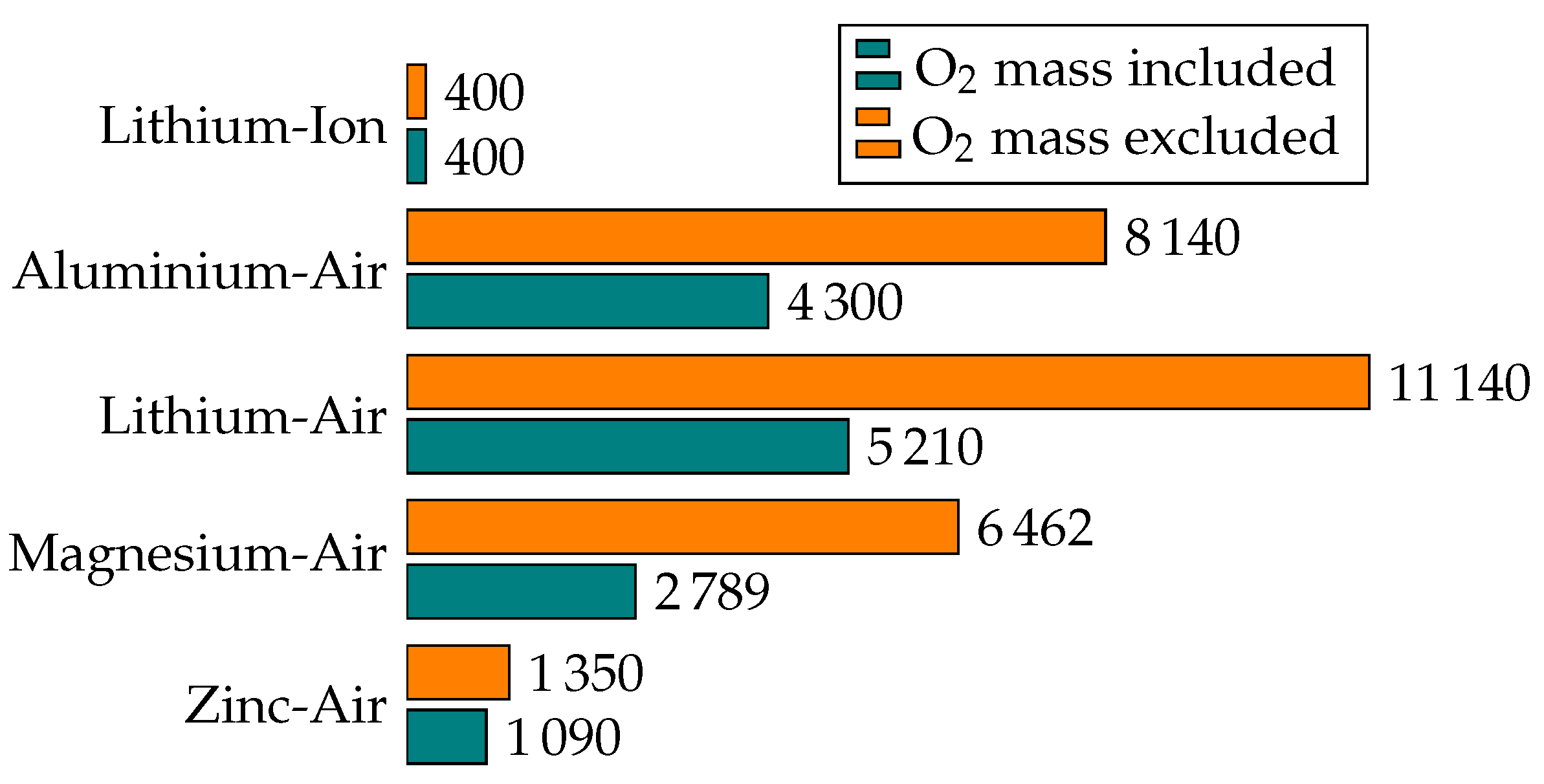
This massive expansion of battery technology cannot be based on existing battery technologies alone for several reasons. First, the raw materials of existing technologies are limited and are mainly found in countries that do not allow safe working conditions. Zinc, on the other hand, is more often found in countries that do not exploit their employees, such as Australia and North America. Another point concerning raw materials is the recyclability cycle. The simple construction of zinc–air batteries helps here. They can be opened without danger and the components can be separated without great effort. Secondly, the theoretical energy density of metal–air batteries is much greater than existing battery technologies. For example, the theoretical energy density of zinc–air cells is three times greater than that of lithium-ion cells.

However, the operation of zinc–air cells is more complex, as existing BMS cannot be used. The reason for this is the small voltage differences that occur during charging and discharging. State of the art battery technologies typically use the cell voltage to detect the state of charge. When a zinc–air cell is charged, the cell voltage increases by only 40 mV during the charging process, i.e., by an order of magnitude less than in other battery technologies where the cell voltage can be used to detect the state of charge. State of charge detection based on cell voltage is not possible, in particular as the influence of temperature and electrolyte concentration on cell voltage is greater than the state of charge itself. The charging process is further complicated by the fact that an accompanying electrolysis process starts at about the same voltage level as the battery charge voltage when the cell is overcharged. This means that overcharging cannot be detected from the cell voltage. Both overcharging and deep discharging damage the cell. However, when discharging, a large voltage drop occurs towards the end of the discharge process, which can be used to detect the end of discharge. Previously, it was therefore not possible to use zinc–air batteries without coulomb counting. The typical application scenarios are excluded by this obstacle, as the cell must be operated continuously in order not to lose the known SoC due to self-discharge. In order to take advantage of the benefits of zinc–air batteries, a method has therefore been developed that enables the detection of the state of charge.

A very promising method to generate measurement data that depend on the state of charge of the cell is EIS. Here, the impedance of the cell is measured for a whole set of different frequencies. However, the unique electrode arrangement of zinc–air secondary cells means that conventional EIS measurement systems are not suitable for use with zinc–air batteries. Therefore, the development of an adapter board was demonstrated that allows existing EIS measurement systems to be used with zinc–air batteries. As stand-alone EIS measurement systems are usually very large and cost-intensive, a small and low-cost measurement system was developed, which makes the integration of the measurement technology financially attractive even for smaller energy storage systems, such as those used in the private sector for intermediate storage of solar energy.

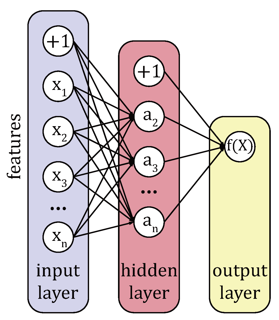
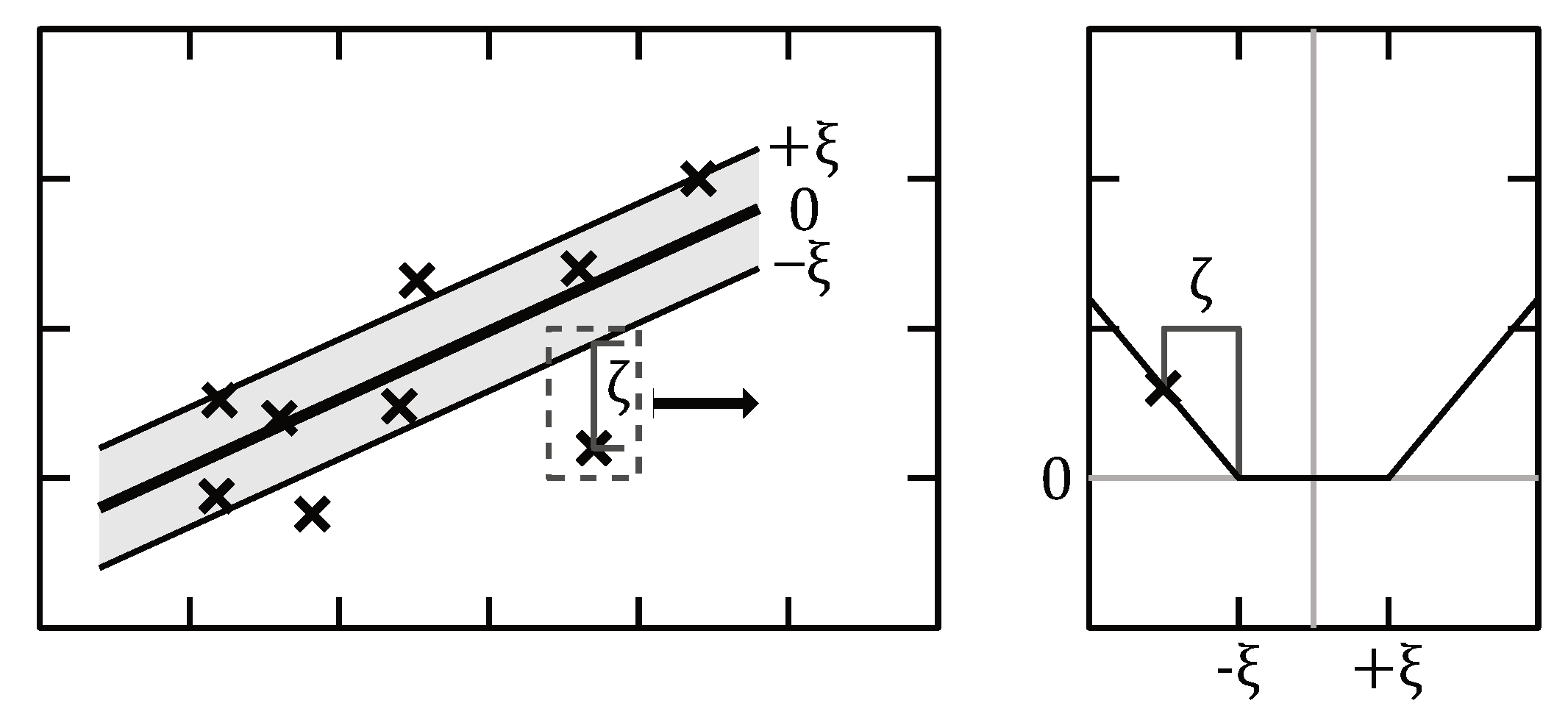
Typically, the measured impedance spectra are used to parameterize an electrical equivalent circuit of the battery. However, many of the components of the equivalent circuit depend not only on the frequency but also on the operating point or the DC current component during the impedance measurement. Therefore, an exact knowledge of the cell processes is necessary to work out the influence of the DC current on the parameters. Typically, previous approaches therefore assume a fixed operating state of the cell while the measurement data are being recorded. In the article, methods of machine learning, were also used to check the capability of determining the state of charge on the basis of the EIS spectra measured at different charging currents. Artificial neural networks and SVR turned out to be particularly promising. In contrast to the common process of parameter fitting, both methods use the raw measured data of the measured impedance spectra as input data, so an exact knowledge of the battery model is not necessary and they can be applied particularly easily. The hyperparameters of the two methods were optimized in the grid search procedure and via a Bayesian optimization on the basis of the training data set in order to prevent data leakage.

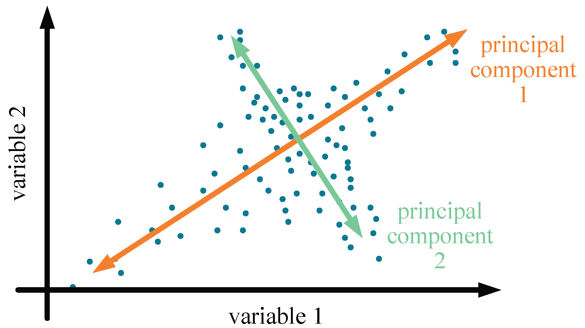
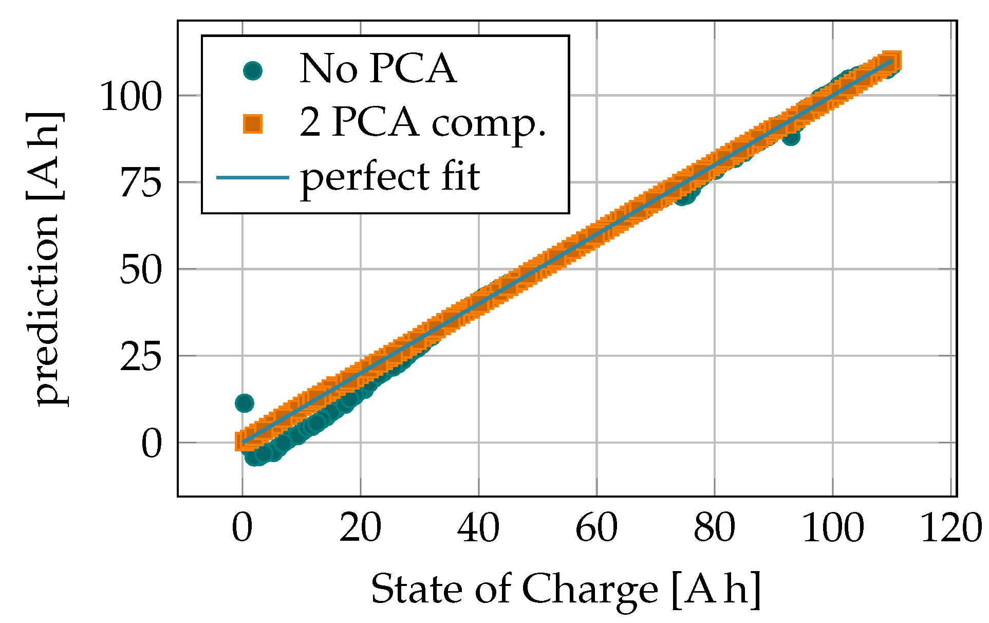
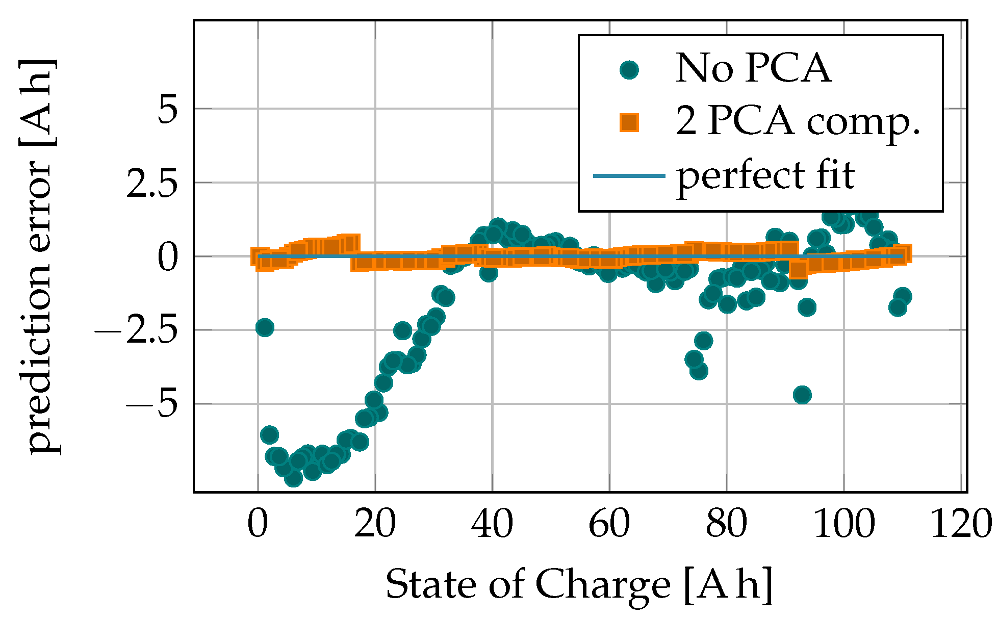
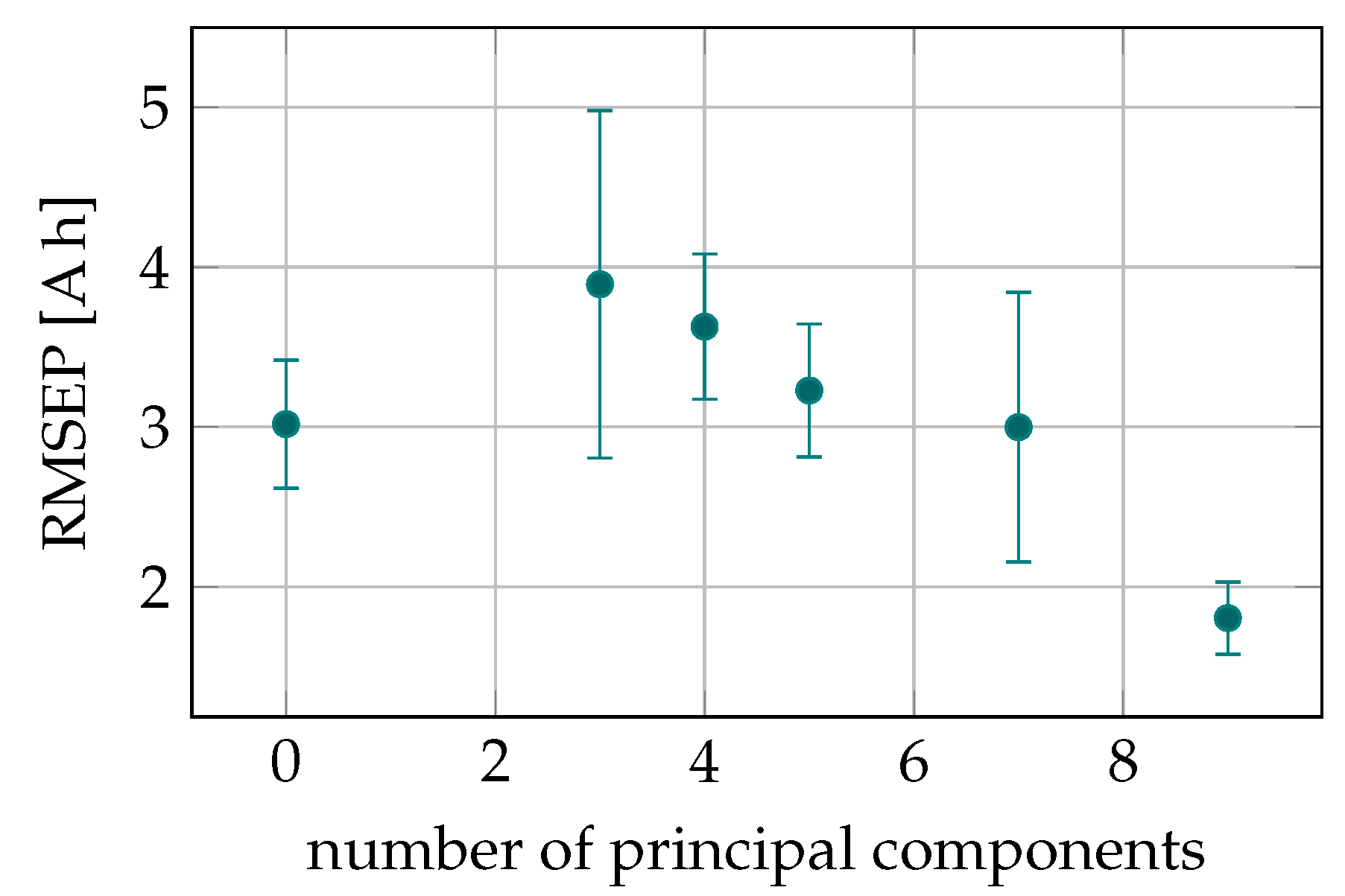
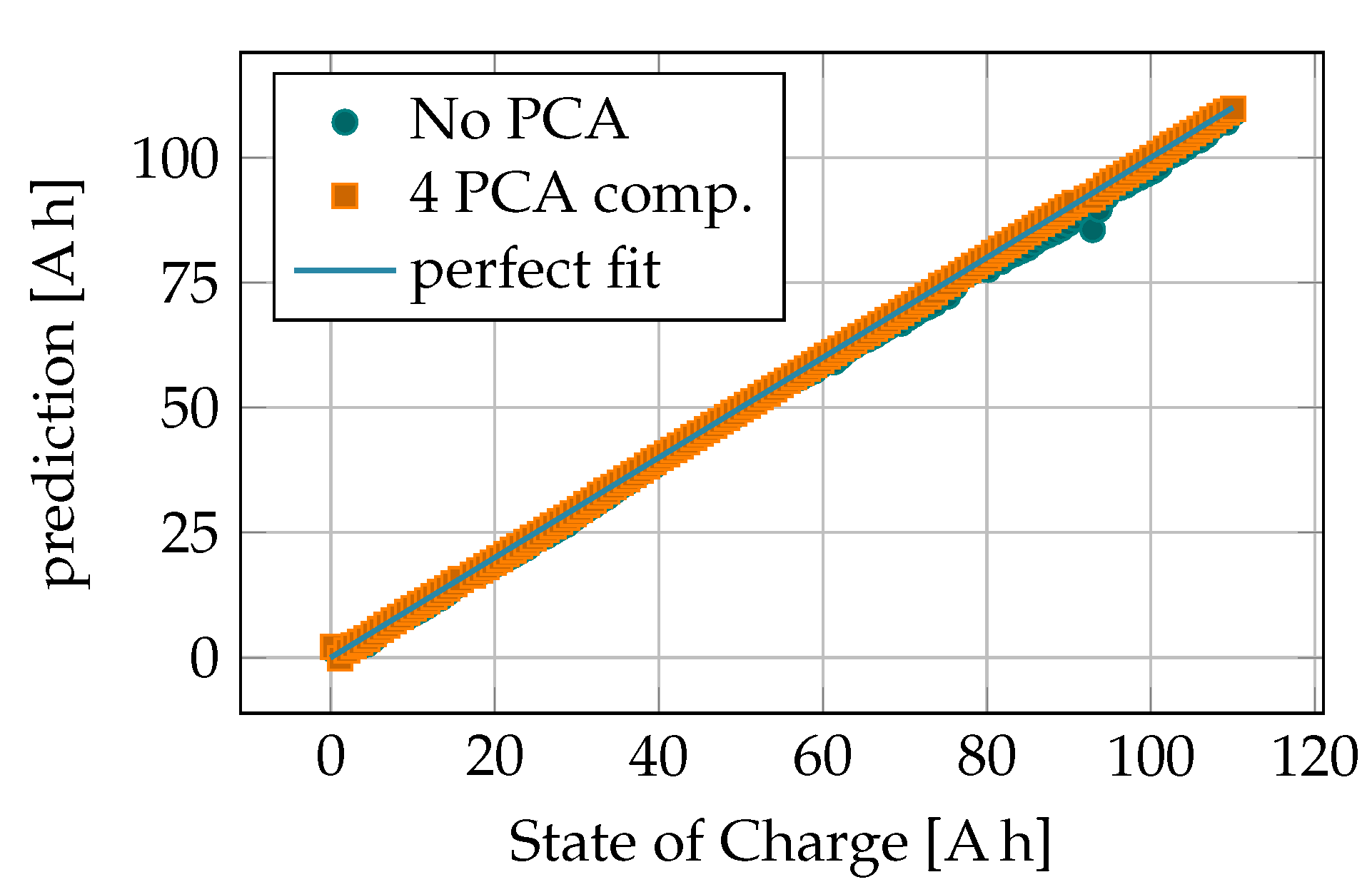
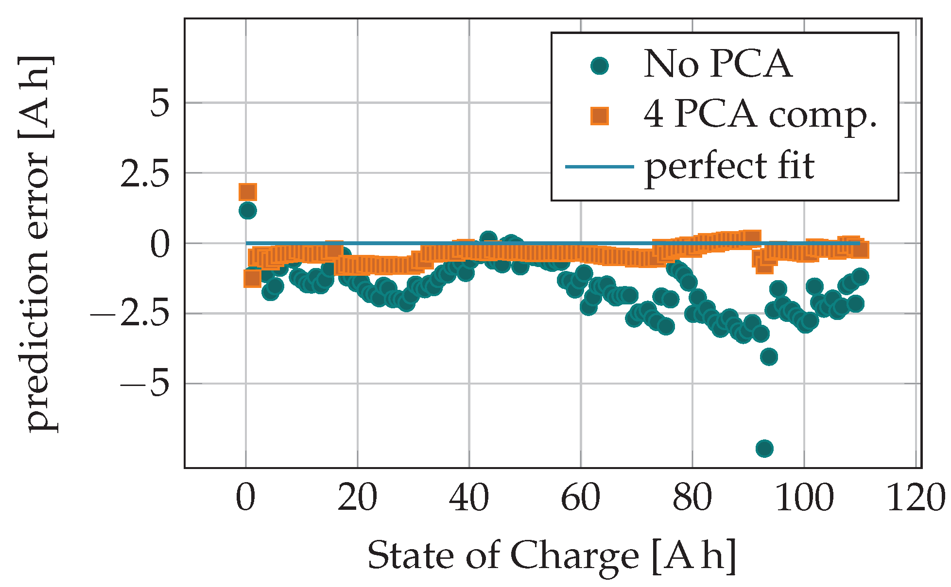
A crucial point and a highlight is that both artificial intelligence methods can also be applied to unknown DC currents during impedance measurement. A change in the charge or discharge current, for example, leads to a change in the linearized charge transfer resistance and thus to different impedance spectra. Provided that the training data contains the charging current selected from the outer limits of possible charging currents, the determination of the state of charge when interpolating the charging current within these limits is very precise. In principle, both methods are sufficiently accurate. By means of a principal component transformation, the dimensionality of the feature space was reduced with very little loss of information. Provided that a particularly strong reduction in the dimensionality is used, ANN show a better performance. Thus, the RMSEP is smaller when using one to four principal components inclusive than with SVR. The best result is obtained when using two principal components. With a higher dimensionality of the input data the SVR is ahead. Even when the principal component transformation is not used, SVR shows a smaller tendency to overfit, so that the metric is only about half as large. When considering the best results, the ANN achieves an error of 0.16% and the SVR achieves an error of 0.47% on unseen data.

In practice, this success is of great relevance. Now, no predefined charge current is needed, which was trained beforehand. Thus, the current working point of the battery does not have to be left in order to start the determination of the state of charge, as long as the dc current is within the trained limits.

References

1. Bundesministerium für Umwelt. Altbatterien. 2020. Available online: www.umweltbundesamt.de (accessed on 15 March 2021).
2. Bundesministerium für Wirtschaft and Bundesministerium fuer Bildung und Forschung. Plattform Industrie 4.0—Was ist Industrie 4.0. 2021. Available online: www.plattform-i40.de (accessed on 27 September 2021).
3. Transport and Environment Reporting Mechanism. Transport: Increasing Oil Consumption and Greenhouse Gas Emissions Hamper EU Progress towards Environment and Climate Objectives; Technical Report 15/2019; European Environment Agency: Copenhagen, Denmark, 2020. Available online: www.eea.europa.eu (accessed on 27 September 2021).
4. Zentrum für Sonnenenergie- und Wasserstoff-Forschung Baden-Württemberg (ZSW). Bestand an Elektro-Pkw Weltweit. 2021. Available online: www.zsw-bw.de (accessed on 18 March 2021).
5. Regelous, A.; Meyn, J.P. Erneuerbare Energien—Eine physikalische Betrachtung. Didaktik Physik 2011, 19, 1–5. [Google Scholar]
6. Quaschning, V. Regenerative Energiesysteme Technologie—Berechnung—Simulation, 9th ed.; Carl Hanser Verlag: Munich, Germany, 2015. [Google Scholar]
7. Knorr, K. Abschätzung der Netzstabilität einer rein Regenerativen Stromversorgung; Fraunhofer Institut für Windenergie und Energiesystemtechnik IWES: Kassel, Germany, 2012; p. 12. [Google Scholar]
8. Hirst, E. Price-Responsive Demand as Reliability Resources. Consult. Electr.-Ind. Restruct. 2002, 139, 34–41. [Google Scholar]
9. Fraunhofer IEE; Knorr, K. Kombikraftwerk 2. 2013. Available online: www.kombikraftwerk.de (accessed on 19 April 2021).
10. U.S. Department of Energy. Energy Storage Database. 2021. Available online: www.sandia.gov (accessed on 20 April 2021).
11. Greenwood, N.N.; Earnshaw, A. Chemie der Elemente, 1st ed.; VCH: Weinheim, Germany, 1988. [Google Scholar]
12. Breuer, H. Dtv-Atlas Chemie, 9th ed.; Deutscher Taschenbuch Verlag (dtv): München, Germany, 2000; Volume 1. [Google Scholar]
13. Binder, H.H. Lexikon der Chemischen Elemente—Das Periodensystem in Fakten, Zahlen und Daten; S. Hirzel Verlag: Stuttgart, Germany, 1999. [Google Scholar]
14. finanzen.net GmbH. finanzen.net Rohstoffe. 2021. Available online: www.finanzen.net (accessed on 22 April 2021).
15. Abraham, K.M. Rechargeable Batteries for the 300-Mile Electric Vehicle and Beyond. ECS Trans. 2019, 41, 27–34. [Google Scholar] [CrossRef]
16. Li, Y.; Lu, J. Metal-Air Batteries: Future Electrochemical Energy Storage of Choice? ACS Energy Lett. 2002, 2, 1370–1377. [Google Scholar] [CrossRef]
17. Hartmann, P.; Bender, C.L.; Vračar, M.; Dürr, A.K.; Garsuch, A.; Janek, J.; Adelhelm, P. A rechargeable room-temperature sodium superoxide (NaO2) battery. Nat. Mater. 2013, 12, 228–232. [Google Scholar] [CrossRef]
18. Canepa, P.; Sai Gautam, G.; Hannah, D.C.; Malik, R.; Liu, M.; Gallagher, K.G.; Persson, K.A.; Ceder, G. Odyssey of Multivalent Cathode Materials: Open Questions and Future Challenges. Chem. Rev. 2017, 117, 4287–4341. [Google Scholar] [CrossRef]
19. Sandhu, S.S.; Brutchen, G.W.; Fellner, J.P. Lithium/air cell: Preliminary mathematical formulation and analysis. J. Power Sources 2007, 170, 196–209. [Google Scholar] [CrossRef]
20. Li, Y.; Dai, H. Recent advances in zinc-air batteries. Chem. Soc. Rev. 2014, 43, 5257–5275. [Google Scholar] [CrossRef] [Green Version]
21. Brinker, M.P. Strategische Vermarktungsanalyse Eines Zink-Luft-Akkumulators zur Speicherung von Solarstrom. Bachelor’s Thesis, University of Applied Sciences Muenster, Steinfurt, Germany, 2017. [Google Scholar]
22. Greßhoff, M. Wirtschaftlichkeitsanalyse von Zink-Luft-Akkusim Vergleich zu Lithium-Ionen-Akkus für Zukünftige Energiespeicher. Master’s Thesis, University of Applied Sciences Muenster, Steinfurt, Germany, 2021. [Google Scholar]
23. Fachverband Batterien. Anforderungen an Batterie-Entladeanzeiger für Blei-Antriebsbatterien zur Erreichung einer hohen Wirtschaftlichkeit. 2008. Available online: www.zvei.org (accessed on 27 April 2021).
24. Spotnitz, R.; Franklin, J. Abuse behavior of high-power, lithium-ion cells. J. Power Sources 2003, 113, 81–100. [Google Scholar] [CrossRef]
25. Finegan, D.P.; Scheel, M.; Robinson, J.B.; Tjaden, B.; Hunt, I.; Mason, T.J.; Millichamp, J.; Di Michiel, M.; Offer, G.J.; Hinds, G.; et al. In-operando high-speed tomography of lithium-ion batteries during thermal runaway. Nat. Commun. 2015, 6, 6924. [Google Scholar] [CrossRef]
26. Murnane, M.; Ghazel, A. A Closer Look at State of Charge (SOC) and State of Health (SOH) Estimation Techniques for Batteries. 2017. Available online: www.analog.com (accessed on 19 December 2020).
27. Nernst, W. Die Elektromotorische Wirksamkeit der Jonen; Wilhelm Engelmann: Wilhelm, Germany, 1889. [Google Scholar] [CrossRef]
28. Schule, J.; Drossbach, P. Elektrochemische Untersuchungen an Kohleelektroden I—Die Ueberspannung des Wasserstoffs. Electrochim. Acta 1964, 9, 1391–1404. [Google Scholar] [CrossRef]
29. Arai, H.; Mueller, S.; Haas, O. AC Impedance Analysis of Bifunctional Air Electrodes for Metal-Air Batteries. J. Electrochem. Soc. 2000, 147, 3584. [Google Scholar] [CrossRef]
30. Ran, L.; Junfeng, W. Prediction of state of charge of Lithium-ion rechargeable battery with electrochemical impedance spectroscopy theory. In Proceedings of the 2010 5th IEEE Conference on Industrial Electronics and Applications, Taichung, Taiwan, 15–17 June 2010; p. 5. [Google Scholar]
31. Loechte, A.; Gebert, O.; Heming, D.; Kallis, K.T.; Gloesekoetter, P. State estimation of zinc air batteries using neural networks. Neural Comput. Appl. 2018, 32, 369–377. [Google Scholar] [CrossRef]
32. Barsoukov, E.; Macdonald, J.R. (Eds.) Impedance Spectroscopy: Theory, Experiment, and Applications, 3rd ed.; Wiley: Hoboken, NJ, USA, 2018. [Google Scholar]
33. Kiel, M. Impedanzspektroskopie an Batterien unter Besonderer Berücksichtigung von Batteriesensoren für den Feldeinsatz; Number 67 in Aachener Beiträge des ISEA; Shaker: Aachen, Germany, 2013; OCLC: 852507405. [Google Scholar]
34. Goertzel, G. An Algorithm for the Evaluation of Finite Trigonometric Series. Am. Math. Mon. 1958, 65, 34. [Google Scholar] [CrossRef] [Green Version]
35. Mcculloch, W.S.; Pitts, W. A logical calculus of the ideas immanent in nervous activity. Bull. Math. Biol. 1990, 52, 99–115. [Google Scholar] [CrossRef]
36. Rosenblatt, F. The perceptron: A probabilistic model for information storage and organization in the brain. Psychol. Rev. 1958, 65, 386–408. [Google Scholar] [CrossRef] [Green Version]
37. Wilamowski, B. Neural network architectures and learning. In Proceedings of the IEEE International Conference on Industrial Technology, Maribor, Slovenia, 10–12 December 2003; IEEE: Maribor, Slovenia, 2003; pp. TU1–T12. [Google Scholar] [CrossRef]
38. Vapnik, V.N. The Nature of Statistical Learning Theory, 2nd ed.; Statistics for Engineering and Information Science; Springer: New York, NY, USA, 2000. [Google Scholar]
39. Smola, A.J.; Schölkopf, B. A tutorial on support vector regression. Stat. Comput. 2004, 14, 199–222. [Google Scholar] [CrossRef] [Green Version]
40. Aizerman, M.A.; Braverman, E.M.; Rozonoer, L.I. Theoretical foundation of potential functions method in pattern recognition. Avtomat. Telemekh. 1964, 25, 917–936. [Google Scholar]
41. Geladi, P.; Kowalski, B.R. Partial least-squares regression: A tutorial. Anal. Chim. Acta 1986, 185, 1–17. [Google Scholar] [CrossRef]
42. Komijani, H.; Rezaeihassanabadi, S.; Parsaei, M.R.; Maleki, S. Radial Basis Function Neural Network for Electrochemical Impedance Prediction at Presence of Corrosion Inhibitor. Period. Polytech. Chem. Eng. 2016, 61, 128–132. [Google Scholar] [CrossRef] [Green Version]
43. Conesa, C.; Ibáñez Civera, J.; Seguí, L.; Fito, P.; Laguarda-Miró, N. An Electrochemical Impedance Spectroscopy System for Monitoring Pineapple Waste Saccharification. Sensors 2016, 16, 188. [Google Scholar] [CrossRef] [PubMed] [Green Version]
Figure 1. Total sold quantity of device batteries in Germany [1].
Applsci 12 00274 g001
Figure 2. Worldwide new registrations of battery electric vehicles and plug-in hybrids (PHEV) [4].
Applsci 12 00274 g002
Figure 3. Theoretical specific energy of different battery technologies in [ W h   k g 1 ] [16,19].
Applsci 12 00274 g003
Figure 4. Successive charging and discharging of a zinc–air battery with constant current.
Applsci 12 00274 g004
Figure 5. Impedance spectra of zinc-air batteries at different working points and SoCs.
Applsci 12 00274 g005
Figure 6. Used zinc–air cell and schematic structure.
Applsci 12 00274 g006
Figure 7. Schematic of developed circuit for measuring impedance spectra.
Applsci 12 00274 g007
Figure 8. Schematic signal generation.
Applsci 12 00274 g008
Figure 9. Schematic of Sample and Hold component.
Applsci 12 00274 g009
Figure 10. Schematic of the PID current controller.
Applsci 12 00274 g010
Figure 11. Step response of the PID current controller.
Applsci 12 00274 g011
Figure 12. Step response of the PID current controller combined with signal generation unit.
Applsci 12 00274 g012
Figure 13. Control deviation of the PID current controller combined with signal generation unit when applying a step.
Applsci 12 00274 g013
Figure 14. Measured voltage signal of an impedance measurement whose direct component increases during the charging process.
Applsci 12 00274 g014
Figure 15. Adjusted voltage signal of an impedance measurement after subtracting the linear DC voltage function.
Applsci 12 00274 g015
Figure 16. Samples of measured impedance spectra. The frequency range is from 100 m Hz to 10 k Hz .
Applsci 12 00274 g016
Figure 17. Schematic of the electrode changer board used to drive three-electrode technology cells with EISmeter impedance spectroscope.
Applsci 12 00274 g017
Figure 18. Charging cycle at varying charge currents.
Applsci 12 00274 g018
Figure 19. Discharging cycle at varying charge currents.
Applsci 12 00274 g019
Figure 20. General structure of artificial neural networks.
Applsci 12 00274 g020
Figure 21. Penalization of training data with a deviation larger as ϵ .
Applsci 12 00274 g021
Figure 22. Illustration of the principal component transformation.
Applsci 12 00274 g022
Figure 23. RMSEP and standard deviation of crossvalidated training data depending on number of principal components.
Applsci 12 00274 g023
Figure 24. Difference between predicted state of charge values and the actual values of polynomial and radial basis model.
Applsci 12 00274 g024
Figure 25. Difference between predicted state of charge values and the actual values of polynomial and radial basis model.
Applsci 12 00274 g025
Figure 26. RMSEP and standard deviation of crossvalidated training data depending on number of principal components.
Applsci 12 00274 g026
Figure 27. Difference between predicted state of charge values and the actual values of polynomial and radial basis model.
Applsci 12 00274 g027
Figure 28. Difference between predicted state of charge values and the actual values of polynomial and radial basis model.
Applsci 12 00274 g028