MUCPSO: A Modified Chaotic Particle Swarm Optimization with Uniform Initialization for Optimizing Software Effort Estimation

Abstract

Particle Swarm Optimization is a metaheuristic optimization algorithm widely used across a broad range of applications. The algorithm has certain primary advantages such as its ease of implementation, high convergence accuracy, and fast convergence speed. Nevertheless, since its origin in 1995, Particle swarm optimization still suffers from two primary shortcomings, i.e., premature convergence and easy trapping in local optima. Therefore, this study proposes modified chaotic particle swarm optimization with uniform particle initialization to enhance the comprehensive performance of standard particle swarm optimization by introducing three additional schemes. Firstly, the initialized swarm is generated through a uniform approach. Secondly, replacing the linear inertia weight by introducing the nonlinear chaotic inertia weight map. Thirdly, by applying a personal learning strategy to enhance the global and local search to avoid trap in local optima. The proposed algorithm is examined and compared with standard particle swarm optimization, two recent particle swarm optimization variants, and a nature-inspired algorithm using three software effort estimation methods as benchmark functions: Use case points, COCOMO, and Agile. Detailed investigations prove that the proposed schemes work well to develop the proposed algorithm in an exploitative manner, which is created by a uniform particle initialization and avoids being trapped on the local optimum solution in an explorative manner and is generated by a personal learning strategy and chaotic-based inertia weight.

1. Introduction

Software effort estimation (SEE) is an early activity in the software life cycle. SEE estimates the level of effort and the cost required to develop a new software system. Estimating the required effort is essential because software organizations are obligated to release software within a given time frame and within a certain cost. Unfortunately, most software projects are delivered after the deadline and over budget. Time and cost overruns have been common problems in software projects for many years [1]. Hence, the accuracy of estimating effort and cost is an essential factor in SEE to successfully avoid the time and budget overruns for overall software delivery [2,3]. To achieve this goal, during the last decade, efforts to create an estimation method have been proposed using parametric, expert judgement, learning oriented techniques, regression based methods, dynamic based models, and composite methods [4].

In order to formulate a method to achieve an improvement in estimation of effort, efforts are ongoing to produce more accurate and reliable models. Effort estimation is a complex problem, and the attribute relation is difficult to analyse. Therefore, the optimization process plays a crucial role in this regard. Optimization can be directly utilized in the effort estimation process, such as the optimization of attribute weighting in COCOMO, Use Case Points, or Analogy Based Estimation (ABE).

Particle swarm optimization (PSO) is one of Swarm intelligence (SI) algorithms alongside Galactic Swarm Optimization (GSO), the Firefly Algorithm (FA), Ant Lion Optimization (ALO), Ant Colony Optimization ACO, Artificial Bee Colony algorithm (ABC), Whale Optimization, Glowworm Swarm Optimization (GSO), and Cuckoo Search Algorithm (CSA). Swarm intelligence has been widely used in hybrid approaches. For instance, the genetic operators have been hybridized with PSO, such as a standard selection mechanism from evolutionary computations [5], the employment of two different crossover operations in order to breed promising exemplars [6], and an adaptive mutation strategy [7]. Similarly, Ant Colony optimization [8], the differential evolution algorithm [9], tabu search [10], Artificial Bee colony [11], Firefly Algorithm [12] and gravitational search algorithm [13] have been incorporated into PSO to take full advantage of each algorithm’s strengths.

Particle Swarm Optimization (PSO) was introduced in 1995 by [14] and gained a high level of interest since it has three advantages: ease of implementation, the requirement of parameters that are simply tuned, and its effectiveness in identifying the global optimum solution since it has a clearer particle direction [15]. Due to its benefit, PSO is widely used in software effort estimation research [16]. However, it still has some shortcomings, such as premature convergence and being trapped into local optima and a poor global search ability [15]. Premature convergence and poor global search ability are influenced by the inertia weight parameter and acceleration coefficient. Inertia weight (ω) can provide particles with a dynamic adjustment ability in different environments, thus realizing the balance between exploration and exploitation. Inertia weight plays an important role in controlling the processes of exploration (global search) and exploitation (local search) by maintaining a balance in their capabilities. From the perspective of statistical analysis, it is believed that the overall performance of PSO is strongly affected by the inertia weight [17].

Researchers have provided various modified versions of PSO to overcome the flaws. Generally speaking, there are six strategies to achieve these goals, such as tuning the following control parameters: inertial weight (w) [18], cognitive acceleration coefficient ($c_1$) and social acceleration coefficient ($c_2$) [19]; hybrid PSO [13]; changing topological structure [20], eliminating the velocity formula [21]; changing the learning strategy [22]; and changing particle initialization strategy [23]. These variants have successfully improved PSO performance.

Although numerous optimization algorithms have been successfully applied to the parameter extraction of software effort estimation systems, it is still indispensable to introduce a novel algorithm to achieve higher accuracy and consequently, improve the total efficiency of different estimation methods. Accordingly, the main objective of this study is to extract the parameters of the various effort estimation methods by exploiting the importance of merging uniform initialization, chaotic mapping, and a personal learning strategy with PSO algorithm.

The purpose of proposed PSO variant is to obtain good performance by addressing the premature convergence and trap into local optima drawbacks. However, the challenges of premature convergence and easy trapping in the local optimum solution still persist. Therefore, in this research, a modified chaotic-based PSO with uniform particle initialization (MUCPSO) is proposed to enhance the comprehensive performance of the standard PSO algorithm. The MUCPSO balances the global and local search to enhance the diversity of initial swarm by forming them dispersedly while avoiding premature convergence by introducing three additional schemes. Firstly, initialized particle or swarm initialization is generated by uniform approach. Secondly, the linear inertia weight is replaced by an introduction of the nonlinear chaotic inertia weight map. Thirdly, a personal learning strategy to enhance the global and local search to avoid trap in local optima. The MUCPSO is finally examined and compared with standard PSO (SPSO) [14], and the following two latest PSO variants: chaotic based PSO (CPSO) [24], uniform chaotic initialized PSO (UCPSO) [23], and one nature-inspired optimization, i.e., Genetic Algorithm (GA) [25] by using three software effort estimation methods as the benchmark functions: Use Case Points, Agile, and COCOMO.

One main contribution of this study is the improvement of the standard PSO by introducing three parameters such as the uniform approach for the diversity of particle initialization, nonlinear chaotic inertia weight map to balance between the exploration and exploitation phase, and personal learning strategy to enhance the global and local search in order to avoid trapping in local optima.

The remainder of this paper is arranged as follows: Section 2 present a related work; Section 3 presents details of standard particle swarm optimization; Section 4 presents details of MUCPSO as the proposed algorithm; Section 5 details materials and methods; Section 6 presents and discusses the experimental results and Section 7 discuss the conclusion and recommends future works of this study.

2. Related Work

PSO results, especially in convergence speed and quality of a final solution heavily depends on the quality of initial particles or particles initialization [26]. High quality initialized particles are achieved when they are more dispersed and closer to the global minimum. In many existing PSO variants, particles are initialized randomly. Initialization is a critical factor in the PSO algorithm that significantly affects diversity and convergence. Such an initialization has characteristics of slow convergence and become easily trapped in local optima [27]. This drawback is due to the lack of diversity in initialized particles. Hence, studies have been conducted to enhance the diversity of initialized particles. Tent or Logistic chaotic mapping is introduced by [28,29,30,31,32] to initialize uniformly distributed particles. This chaotic-based initialization achieved better results compared with random-based initialization. Refs. [33,34] proposed an opposition-based population initialization by employing a symmetric strategy. This strategy can prevent initial particles from being distant from the global optimum. Opposition-based learning (OBL) is also employed in the work of [26], combined with Logistic chaos mapping. The experiments validate that this kind of initialization can recognize the search area better. Slightly different to others, Rehman [35] uses semi-random initialization by dividing the entire search space. The distribution of particles over a search space is performed in independents slots. The Weibull probability sequence is used to generate numbers at random locations for swarm initialization [36]. In the most recent study, Zhang [23] introduced uniform initialization (UI) strategy. UI strategy initializes a particle randomly as the basic point and then generates other initial particles based on this basic point. Hence, the initial particles are evenly distributed in each dimension, and the positions of each particle in each dimension are randomized. This mechanism can prevent the aggregation of initial particles. Ref. [37] proposed a pseudo-random initialization strategy called WELL on population initialization. This strategy imparted a significant effect on the importance of convergence and diversity.

Maintaining a balance between exploration and exploitation is very important for an optimization algorithm. In this way, inertia weight plays a critical role to maintain this balance. In standard PSO (SPSO), inertia weights are based on linear decreasing weight, which lead to a poor result/balance. Therefore, several studies have been proposed to tackle this problem. Refs. [38,39], proposed random-based inertia weights. This kind of randomness improved the population diversity in the early search phase, while it affects the local search ability in the later search phase, which reduces the convergence speed. In contrast, Zhang [40] and Sedighizadeh [41] introduced a dynamic inertia weight to replace the random inertia weight by controlling the convergence of the swarm towards a solution. An adaptive inertia weight based on the binomial probability distribution is proposed by [18], while [42] using the triangular probability density function to make the inertia weight generally greater in the initial stage of evolution, which is suitable for global search. Ref. [43] proposed an adaptive self-inertia weight with a gradient-based local search strategy. As stated by [44], for better performance, the inertia weight should be nonlinearly and dynamically changed to achieve better dynamics of balance between global and local search abilities. Recent studies proposed a chaotic-based inertia weight strategy. Ref. [45] used Sine map [46], Gauss map, and [47] Logistic map to adjust and tune the inertia weight.

In SPSO, the velocity and position of each particle are updated using a learning mechanism based on its personal and population best experience. This learning mechanism is simple and easy to implement, but it suffers from some potential problems, such as the phenomena of “oscillation” and “two steps forward, one step back” as coined by [48]. Thus, several studies proposed improvements such as the dimensional learning strategy introduced by [48] by introducing a two-swarm learning PSO (TSLPSO) algorithm based on different learning strategies. One of the subpopulations constructs the learning exemplars by DLS to guide the local search of the particles, and the other subpopulation constructs the learning exemplars by the comprehensive learning to guide the global search. The dimension-based velocity updating equation proposed by [40] also divides the population into two particle-based updating equations with the two approach, and the two are executed alternately to form a novel social learning PSO. Unlike SPSO learning strategies, where the particles are updated based on historical information, each particle in the Social learning PSO [40] is able to learn from better particles in the same swarm. Dynamic learning strategy is proposed by [49] by promoting information exchange among sub-swarms, ordinary particles and communication particles. The ordinary particles focus on exploitation under the guidance of the local best position in its sub-swarm, while the communication particles have a dynamic ability and focus on exploration under the guidance of a united local best position in a new search region to promote information exchange among sub-swarms. The adaptive learning strategy proposed by [50] employed a self-learning based candidate generation strategy to ensure the exploration ability, and a competitive learning (CL) based prediction strategy to guarantee exploitation of the algorithm, while [51] used adaptive mechanism for adjusting comprehensive learning probability and a cooperative archive (CA) combined with standard PSO. Ref. [47] proposed a stochastic and mainstream learning strategy to replace the personal and global learning strategies. Stochastic learning allows particles to learn from other excellent particles in the population, making the movement of particles more diverse. By enhancing the diversity of the population, the premature convergence of SPSO is managed. Lately, Zhou [52] proposed local minimum early warning to reflect the risk of being trapped in a local minimum. It determines the paradigm evolution direction and adjusts the trajectory of particles in different risk environments. In order to improve the ability to resist the temptation of local optima, the adaptive hierarchical update method generates two-layer and three-layer update formulas for the global exploration subpopulation and the local exploitation subpopulation, respectively.

3. Standard Particle Swarm Optimization

Standard article swarm optimization (SPSO) is inspired by the behavior of bird flocking and fish schooling to find a place with enough food [28]. Algorithm 1 describes the process of SPSO. This algorithm starts by randomly generating the populations based on the swarm size parameter. The population consists of N particles in which each particle i acts as the representation of potential solutions to the given problem. A particle is represented by the vector x_i in the decision space. Each particle has its position (x) and velocity (v). Position represents the flying direction, and velocity relates to the step of the particle.

The cooperation between particles achieves optimization. The particle closest to the objective is called the success particle. The success particle will influence the behavior of other particles. They will adjust their positions ($x_i$) toward the global optimum. Two factors affect the position of the particle. First, the best position visited by itself called personal best ($Pbes{t}_i$), and second, the best position visited by the particles overall, known as the global best ($Gbes{t}_i$).

After the population is successfully created, for the following iterations, each particle will apply the following operations:

First, update the velocity to define the amount of change applied to the particle as formulated in Equation (1).

$$v_{i+1}=\omega v_i+C_1{R}_1\ast \left(Pbes{t}_i-x_i\right)+C_2{R}_2\ast \left(Gbes{t}_i-x_i\right)$$

(1)

where $v_{i+1}$ is a new velocity, and $v_i$ is current or initialized velocities. Initialized velocity means that $v_i$ is assigned as a random number between 0 and 1 alongside the generation of the population. $C_1$ and $C_2$ represent the constant variables that are well known as cognitive learning factors and social learning factors. $R_1$ and $R_2$ are random variables in the range of [0,1]. $Pbes{t}_i$ is the best position visited by particle i. $Gbes{t}_i$ is the best position visited by overall particle. $x_i$ is the current position of particle, whereas ω is an inertia weight (see Equation (2)), where ${\omega }_t$ is inertia weight of current iteration t, ${\omega }_{max}$ is maximum inertia value equal to 0.9, ${\omega }_{min}$ is minimum inertia value equal to 0.4, and $T_{max}$ is the maximum iteration.

Inertia weight controls the momentum of the particle by weighting the contribution of the previous velocity, controlling the extent to which the previous flight direction will influence the new velocity. Inertia weight is critical in ensuring convergent behavior as formulated in Equation (2).

$${\omega }_t={\omega }_{max}+\frac{\left({\omega }_{max}-{\omega }_{min}\right)\ast t}{T_{max}}$$

(2)

Second, the position of the particle is updated as notated in Equation (3), where $x_{i+1}$ is a new position of the particle, $x_i$ is the last position, and $v_i$ is the current velocity of the particle.

$$x_{i+1}=x_i+v_i$$

(3)

Each particle will update their personal best solution if $x_i<Pbes{t}_i$ then $Pbes{t}_i=x_i$ and the global best will be updated if $x_i<Gbes{t}_i$, then $Gbes{t}_i=x_i$.

Algorithm 1. Standard Particle Swarm Optimization algorithm (SPSO).

(1)  Input: Dataset X, Parameters settings in Table 4 (2)  Output: Optimized solutions (3)  for each project in X do (4)  generate initial population (5)  while (Gbest > stopping value) or (Tmax > 0) do (6)      for i = 1, 2, 3, …, Tmax do (7)        update velocity using Equation (1) (8)        update positions using Equation (3) (9)        calculate effort estimation (10)         updated particles (11)      end for (12)      Gbest ← min(Pbests) (13)      if Gbest > stopping value then (14)       temps[] ← Gbest (15)      else (16)      Gbest (17)      end if (18)      increment++ (19)   end while (20)   if temps is not empty then (21)     Gbest ← min(temps) (22)   end if (23)  end for

4. A Modified Chaotic Based PSO with Uniform Initialization

Inspired by research on particle initialization, inertia weight, and learning strategy, we proposed a new competitive PSO variant called MUCPSO. MUCPSO combines three strategies, and their details are represented in the following sections.

4.1. Uniform Initialization

Random initialization, chaotic initialization, and opposition-based initialization experience challenges in avoiding the aggregation of initial particles. To solve this problem, a uniform initialization strategy [23] is employed. As shown in Algorithm 2, the first line of code initializes a particle randomly as the base point, and $X_1=\left[X_{11},X_{12},\dots ,X_{1D}\right]$ is the position of the base point. Lines 2–4 generate a $D\ast \left(n-1\right)$ random matrix $R=\left[R_1,R_2,\dots ,R_D\right]$ to ensure the randomness of the initial particles. Lines 5–12 divide the length of each dimension by n to obtain the minimum distance between particles in the corresponding dimension. Lines 5–12 distribute particles in each dimension uniformly and avoid the aggregation of particles. If the position of a particles exceeds the allowed range of a dimension, it will subtract the range of the corresponding dimension.

Uniform initialization ensures that the distance between particles is greater than a certain value. It can avoid the aggregation of particles and distribute the initial particle uniformly to recognize more areas at the beginning.

Algorithm 2. Uniform particle initialization algorithm.

(1)  Initialize X1 in the search area randomly (2)  for d = 1 to D do (3)  randomly rearrange [1, 2, …, (n−1)] to get Rd = [R1d, R2d, …, R(n−1)d] (4)  end (5)  for i = 1 to n do (6)  for d = 1 to D do (7)    Xid = X1d + R(i−1)d ÷ n * (Xdmax − Xdmin) (8)    if Xid > Xdmax then (9)      Xid = Xid − (Xdmax − Xdmin) (10)    end (11)  end (12)  end for

4.2. Chaotic Inertia Weight, R₁, and R₂ Parameters

In the SPSO algorithm, there are two parameters that control the trade-off between exploration and exploitation, $R_1$ and $R_2$. $R_1$ and $R_2$, that regulate the movement of particles towards the personal previous bests and global best positions. Consequently, if these two parameters have large values, they supervise or drive the particles to augment the current solution by moving towards the best and global positions, respectively. In contrast, if these parameters raise the small values, they supervise/drive the particles capabilities in exploration. $R_1$ and $R_2$ values are assigned by random value between 0 and 1. In our proposed method, we replaced the random value between 0 and 1 by using a chaotic number between 0 and 1, as formulated in Equation (4). The chaotic maps are able to adapt between the exploitation and exploration phases.

$$\omega \left(t\right)=r\left(t\right).{\omega }_{min}+\frac{\left({\omega }_{max}-{\omega }_{min}\right)\ast t}{T_{max}}, r\left(0\right)=0.7$$

(4)

where $r\left(t\right)$ is a random number generated by the selected chaotic map function. r(0) is defined as 0.7 due to the robust result [46].

There are eight well-known randomness non-linear chaotic maps, as described in

Table 1. Eight well-known chaotic maps.

Map	Function	Range
Gauss	$x_{k+1}=\left\{\begin{array}{cc}\hfill 0, & x_k=0\hfill \\ \hfill \frac{1}{x_k}mod 1, & x_k\ne 0, x_0=0.7\hfill \end{array} \right.$	(0,1)
Singer	$x_{k+1}=1.07\left(7.86x_k-23.3x_k^2+28.75x_k^3-13.3x_k^4\right)$	(0,1)
Logistic	$x_{k+1}=4x_k\left(1-x_k\right)$$, x_0\notin \left(0.0, 0.25, 0.5, 0.75, 1.0\right)$	(0,1)
Circle	$\begin{array}{c}\hfill x_{k+1}=x_k+b-\left(\frac{a}{2\pi }\right)\sin \left(2\pi x_k\right)mod\left(1\right)\hfill \\ \hfill x_{k+1}=x_k+b-\left(a-2\pi \right) \sin \left(2\pi x_k\right)mod\left(1\right)\hfill \\ \hfill \text{where} a=0.5, b=0.2, \mathrm{and} \mathrm{the} \mathrm{chaotic} \mathrm{generate} \mathrm{sequence} \mathrm{is} \mathrm{in} \left(\mathrm{0,1}\right)\hfill \end{array}$	(0,1)
Sine	$x_{k+1}=\frac{a}{4}\sin \left(\pi x_k\right)$, $0<a\le 4$	(0,1)
Sinusoidal	$\begin{array}{c}\hfill x_{k+1}=a{x}_k^2\sin \left(\pi x_k\right)\hfill \\ \hfill \text{where} a=2.3, and x_0=0.7. \mathrm{It} \mathrm{has} \mathrm{the} \mathrm{following} \mathrm{simplified} \mathrm{form}\text{:} x_{k+1}=\sin \left(\pi x_k\right)\hfill \end{array}$	(0,1)
Chebyshev	$x_{k+1}=\cos \left(k co{s}^{-1}\left(x_k\right)\right)$	(−1,1)
Bernoulli shift	$x_{k+1}=\left\{\begin{array}{c}\frac{x_k}{1-\lambda },0<x_k\le 1-\lambda \\ \frac{x_k-\left(1-\lambda \right)}{\lambda },1-\lambda <x_k<1\end{array}\right.$ where $\lambda =1/2$ as treated in [20].	(0,1)

.

For visualization purposes, Figure 1 provides the chaotic value distribution of 100 iterations for all eight maps with random initial values. The vertical (x) axis denotes the iteration number, and the horizontal (y) axis denoted the inertia weight. For a robust result, 0.7 is assigned as the $x_0$ value for all chaotic map functions [46].

4.3. Personal Learning Strategy

Alongside social learning (R₁) and cognitive learning (R₂), velocity updating is also affected by personal and global learning strategies. In practice, the particles learn from their personal best (Pbest) and global best (Gbest) positions. The advantage of this learning strategy means PSO has certain benefits such as fast convergence, high reliability and strong global exploration ability. However, behind the fast convergence remains one drawback, which is premature convergence. To overcome this drawback, we utilized the stochastic personal best (SPbest) as proposed by [47]. SPbest allows the particles to learn from other excellent individuals in the population and makes the movement of particles more heterogeneous. By enhancing the heterogeneity of the population, we are able to overcome the premature convergence in the PSO algorithm. SPbest is, however, contradictive with standard Pbest, for which particles learn only from their own best personal best. The overall three combination strategies proposed in this study are described in Algorithm 3.

Algorithm 3. A modified chaotic particle swarm optimization with uniform Initialization algorithm.

(1)  Input: Dataset X, Parameter settings in Table 4 (2)  Output: Optimized solutions (3)  for each project in X do (4)  generate uniform initial population using Algorithm 2 (5)  while Gbest(min(SPbest)) > Stopping value OR (Tmax > 0) (6)  do (7)    rt, R1, R2 = selected chaotic map (8)    ω = inertia weight by Equation (4) (9)    for i = 1, 2, 3, …, Tmax do (10)      Update velocity by Equation (8) (11)      Update positions by Equation (9) (12)      Calculate effort estimation (13)      Updated particles (14)    end (15)    CPbest by Equation (5) (16)    SPbest(CPbest, Pbest) by Equations (6) and (7) (17)    Gbest(min(Pbest)) (18)    if Gbest > Stopping value then (19)      temps[] ← Gbest (20)    else (21)      Gbest (22)    end (23)    increment++ (24)  end (25)  if temps is not empty then (26)    Gbest(min(temps)) (27)  end (28)  end

Equations (5) and (6) express the SPbest technique. SPbest works as follows: first, from the population, two mutually different personal best (Pbest) particles in each iteration are randomly selected. Second, based on their fitness value, these selected Pbest are compared to determine the candidate personal best solution (CPbest). Second, the better CPbest is compared with the current personal best (Pbest_i) (see Equation (6)). As formulated in Equation (6), if CPbest is less than Pbest_i, then Spbest is equal to Cpbest, and Spbest is equal to Pbest_i, otherwise.

$$\begin{gathered} CPbest\left(t\right)=argmin\left\{fit\left(Pbes{t}_a\left(t\right)\right), fit\left(Pbes{t}_b\left(t\right)\right)\right\}, \\ a\ne b\in \left\{1, 2,\dots ,N\right\} \end{gathered}$$

(5)

where CPbest(t) is the candidate personal best solution, $fit\left(Pbes{t}_a\right)$ is fitness value of Pbest_a, $fit\left(Pbes{t}_b\right)$ is fitness value of $Pbes{t}_b$, N is number of particles.

$$SPbes{t}_i\left(t\right)=\left\{\begin{array}{cc}\hfill CPbest\left(t\right)& fit\left(CPbest\right)<fit\left(Pbes{t}_i\right)\hfill \\ \hfill Pbes{t}_i\left(t\right)& otherwise\hfill \end{array}\right.$$

(6)

$$Pbes{t}_i\left(t\right)=argmin\left\{fit(X_i\left(1)\right), fit(X_i\left(2)\right),\dots ,fit(X_i\left(t)\right)\right\}$$

(7)

Based on this recognition, the standard velocity updating in Equation (1) is replaced by Equation (8) where ${\xi }_1$ and ${\xi }_2$ are the chaotic map values.

$$V_i\left(t+1\right)=\omega \left(t\right)V_i\left(t\right)+C_1{\xi }_1\ast \left(SPbes{t}_i\left(t\right)-X_i\left(t\right)\right)+C_2{\xi }_2\ast \left(Gbes{t}_i\left(t\right)-X_i\left(t\right)\right)$$

(8)

$$X_i\left(t+1\right)=X_i\left(t\right)+V_i\left(t+1\right)$$

(9)

5. Materials and Methods

This section presents the dataset used, along with brief descriptions of the software effort estimation methods as the benchmark function.

5.1. Datasets

The characteristics of the chosen datasets highly affect the software effort estimation evaluation. In this study, we used three real datasets: Silhavy [53] for UCP, NASA93 for COCOMO [54], and Agile [55] datasets for Agile software effort estimation, respectively.

5.1.1. Use Case Points

The original UCP framework proposed by Karner [56] consists of seven steps. First, a calculation of the unadjusted actor weighting (UAW) is performed by classifying the actors into three levels of complexity and assigning a weight for each actor based on its complexity as notated in Equation (10).

$$UAW={\displaystyle \sum }_{i=1}^3{W}_i\ast A_i$$

(10)

where W_i is weight factor classified as simple for 1, the average for 2, and complex actor for 3. A_i is a number of actors in the use case diagrams based on the same classification as W_i. Second, the unadjusted use case weighting (UUCW) is calculated by classifying the use case into three levels of complexity and assigning a weight for each actor based on its complexity level as formulated in Equation (11).

$$\mathrm{UUCW}={\displaystyle \sum }_{i=1}^3{W}_i\ast U{C}_i$$

(11)

where $W_i$ is a weight factor which classified as simple (5), average (10), and complex (15) use case, respectively. UC_i is number of transactions counted in use-case specification diagrams based on the same classification as W_i. Alongside the original weight level,

Table 2. The original and modified use case complexity weight level.

Number of Use Case Transactions	Original Weight Level	Modified Weight Level
1–2	5	5.00
3	5	6.45
4	10	7.50
5	10	8.55
6	10	10.00
7	10	11.40
8	15	12.50
9	15	13.60
>10	15	15.00

presents the complexity weight level derived by [57,58].

Third, the unadjusted use case points (UUCP) are calculated as notated in Equation (12). UAW in Equation (10) is used alongside the UUCW in Equation (11) to obtain UUCP.

$$\mathrm{UUCP}=\mathrm{UAW}+\mathrm{UUCW}$$

(12)

Fourth, technical complexity factors (TCF) are calculated. TCF is formulated in Equation (13) by grading (G_i) the thirteen weight factors (W_i) using a score of 0 to 5.

$$\mathrm{TCF}=0.6+\left(0.01\ast {\displaystyle \sum }_{i=1}^{13}{W}_i\ast G_i\right)$$

(13)

Fifth, the environmental complexity factors (ECF) are calculated as notated in Equation (14) by grading (G_i) the eight factors (W_i) using a score of 0 to 5.

$$\mathrm{ECF}=1.4+\left(-0.03\ast {\displaystyle \sum }_{i=1}^8{W}_i\ast G_i\right)$$

(14)

Sixth, the use case points (UCP) are calculated as formulated in Equation (15). UCP is obtained by multiply UUCP in Equation (12) by TCF in Equation (13) and ECF in Equation (14).

$$\mathrm{UCP}=\mathrm{UUCP}\ast \mathrm{TCF}\ast \mathrm{ECF}$$

(15)

Seventh, the estimated effort is calculated as formulated in Equation (16). Estimated effort is obtained by multiply the UCP in Equation (15) with Productivity Factors (PF).

$$\mathrm{Effort}=\mathrm{UCP}\ast \mathrm{PF}$$

(16)

PF is the productivity factor, and it can be set equal to 20 person-hours/UCP, 8.2 person-hours/UCP [59,60], or using the learning productivity ratio as proposed by [61].

5.1.2. COCOMO II

The first version of COCOMO was proposed in 1981 by Boehm [62]. COCOMO separates the cost driver into three facets such as Effort Multiplier (EM), Line of Code (LoC), and Scale Factors (SF). The cost drivers are calculated by an equation to calculate the effort in person month (PM).

$$Effort \left(PM\right)=A\ast Siz{e}^E\ast {\displaystyle \prod }_{i=1}^{17}E{M}_i$$

(17)

$$E=B+0.01\ast {{\displaystyle \sum }}_{j=1}^{5}S{F}_j$$

(18)

As formulated in Equations (17) and (18), the amount of effort in person months, where A and B are the multiplicative and exponential constants, is at a value of 2.9 and 0.91, respectively. Size is measured in Kilo Source Lines of Code (KLOC). While E defines the scaling exponent for effort. EM is the Effort Multipliers where i = 1 to 17 and SF_j is the Scale Factor where j = 1 to 5.

5.1.3. Agile Estimation

The Agile estimation assigns work to an entire team, not an individual. In this section we describe a detailed Agile estimation as referenced in [55]. First, we calculate the effort of a particular User Story as defined in Equation (19).

$$E{S}_i=Complexity\ast Story Size$$

(19)

where complexity is the relative scale of the requirement of the Story or its technical complexity, and story size is an estimate of the relative scale of the work in terms of actual development effort. Second, the sum of effort of all individual user stories for the complete project as formulated is calculated using Equation (20)

$$Effort={\displaystyle \sum }_{i=1}^{n}E{S}_i$$

(20)

where effort is the estimated effort in person-month, and ES_i is the effort of a current User Story. Third, the agile velocity is calculated by Equation (21).

$$Velocity=Distance\ast Time$$

(21)

where Distance is a unit of completed effort and Time is the length of our sprint. Fourth, the Initial or Raw Velocity is calculated in Equation (22).

$$V_i=\frac{Units of completed effort}{Sprint time}$$

(22)

where Sprint time is the number of days in sprint. Fifth, the Friction (FR) as denoted is calculated using Equation (23).

$$FR={\displaystyle \prod }_{i=1}^{4}F{F}_i$$

(23)

where FR is product of all four Friction Factors (FF_i). Sixth, the Dynamic Force (DF) can be calculated in Equation (24).

$$DF={\displaystyle \prod }_{i=1}^{9}V{F}_i$$

(24)

where DF (Dynamic Factor) is a product of all nine variable factors (VF_i). Seventh, deceleration (D) is calculated by the multiplication of FR and DF. Deceleration adjusts the velocity against friction and dynamic forces as formulated in Equation (25).

$$D=FR\ast DF$$

(25)

Absolute error (AE) and mean absolute error (MAE) are the evaluation metrics used in this study. As formulated in Equation (26), AE is the estimation or prediction error, y_i is the ith actual value of the variable being estimated, and ${\widehat{y}}_i$ is the ith estimated value.

$$\mathrm{AE}=\left|y_i-{\widehat{y}}_i\right|$$

(26)

Moreover, as notated in Equation (27), MAE is the mean value of absolute error.

$$\mathrm{MAE}=\frac{1}{n}{{\displaystyle \sum }}_{i=1}^{n}A{E}_i$$

(27)

where n is the number of projects in the data set, and AE_i is the i^th absolute error value.

6. Results and Discussion

In this research, three software effort estimation methods and three data sets are employed to investigate both the exploitation and exploration abilities of the proposed MUCPSO algorithm.

Table 3. Three software effort estimation as benchmark methods.

Methods	Weight Parameters	Range	Dimension
UCP	Simple	[5, 7.49]	3
	Average	[7.5, 12.49]
	Complex	[12.5, 15]
COCOMO	A	[0, 10]	2
	B	[0.3, 2]
Agile	Team position	[0.91, 1]	13
	Process	[0.89, 1]
	Environmental factors	[0.96, 1]
	Team dynamics	[0.85, 1]
	Expected team change	[0.91, 1]
	Introduction to new tools	[0.96, 1]
	Vendor defect	[0.90, 1]
	Team member responsibility	[0.98, 1]
	Personal issue	[0.98, 1]
	Expected delay	[0.96, 1]
	Expected ambiguity	[0.95, 1]
	Expected change	[0.97, 1]
	Expected relocation	[0.98, 1]

illustrates the effort estimation methods with their name, dimensions, and ranges.

6.1. Preliminary Observations

To assess the behaviors in optimizing the three estimation methods, we follow the procedure of tuning the following two parameters of the MUCPSO algorithm: population p and chaotic maps as described in [63]. Here, for each estimation method, 80 experiments are performed using a combination of 10 values of p = 10, 20, 30, 40, 50, 60, 70, 80, 90, 100, and eight chaotic maps = Bernoulli, Chebyshev, Circle, Gauss, Logistic, Sine, Singer, and Sinusoidal, which can be defined as pairs of (10, Bernoulli), (10, Chebyshev), …, (100, Sinusoidal). To reduce the coincidence, 1000 runs were applied to each pair in experiment. The common parameter value of p is finally selected as a fixed-optimum value for all the estimation methods.

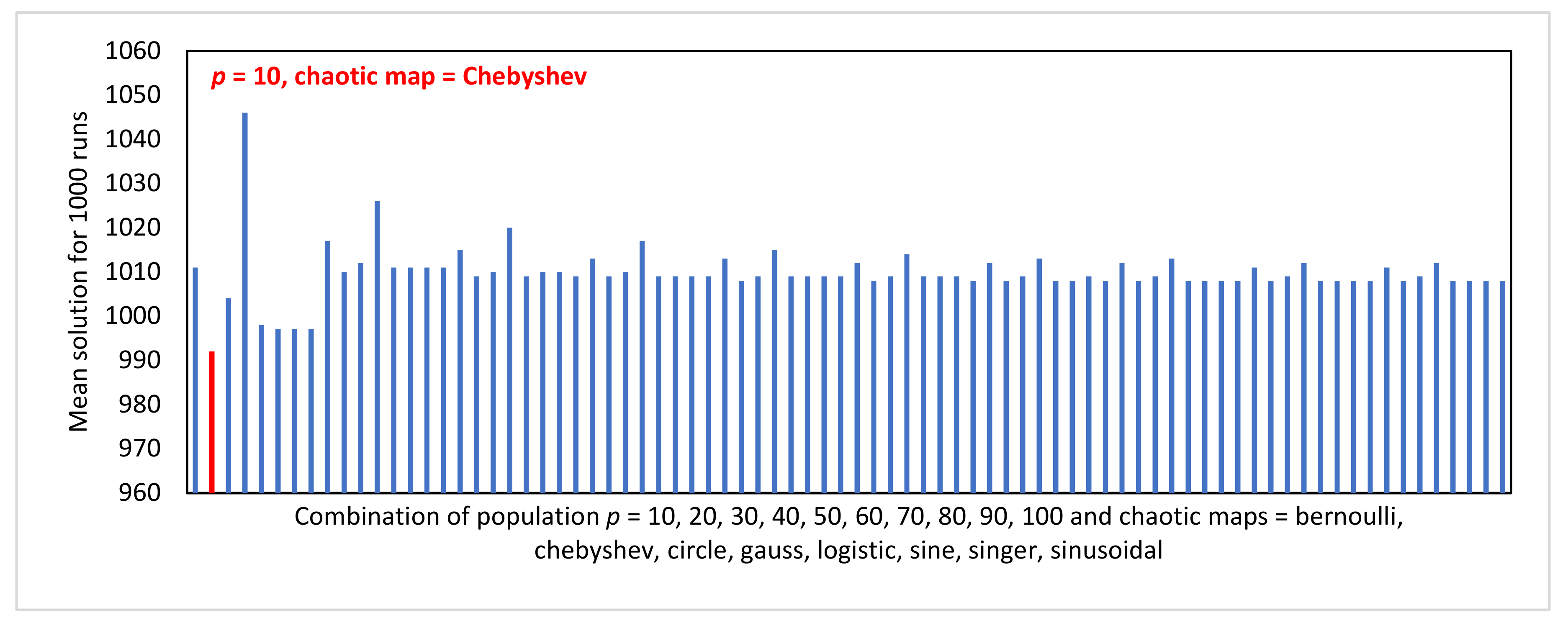
Figure 2 illustrates the experimental results for the problem of searching a minimum solution for the Use Case Points estimation method. The vertical axis shows all results from eighty experiments. It can be seen that a small population p (10) means the MUCPSO produces a good solution. In contrast, the bigger the p, the worse the solution. Hence, the combination of small p and Chebyshev as the chaotic function is recommended. The optimum combination is reached using p = 10 and chaotic = Chebyshev.

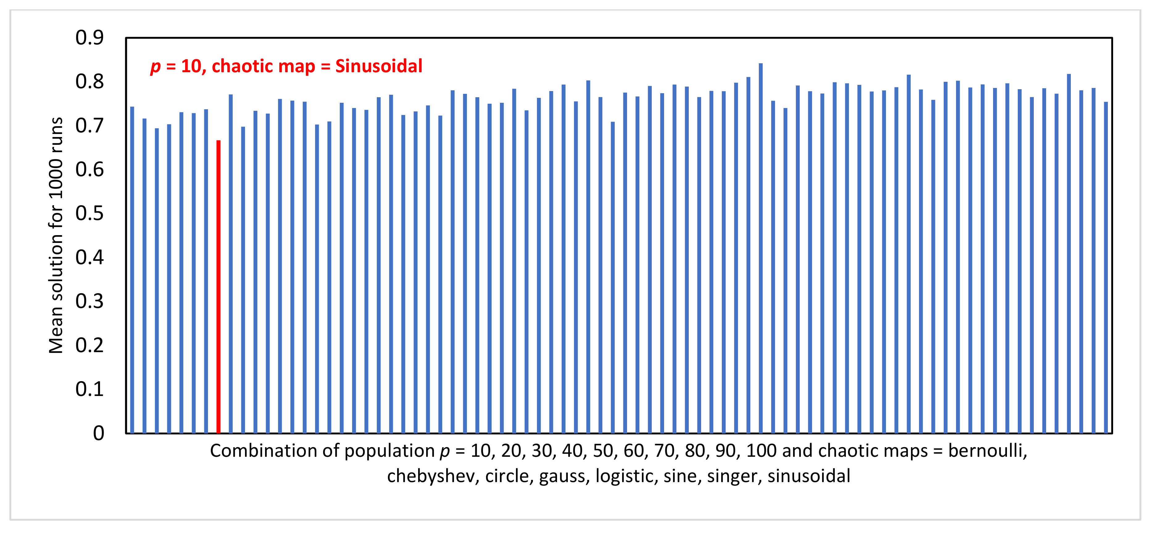
Next, Figure 3 illustrates the experimental results for the problem of searching for a minimum solution in the Agile estimation method. The vertical axis shows all results from eighty experiments. It can be seen that a small population p (10) means the MUCPSO produces a good solution. In contrast, the bigger the p, the worse the solution. Hence, the combination of small p and Sinusoidal as the chaotic function is recommended. The optimum combination is reached using p = 10 and chaotic = Sinusoidal.

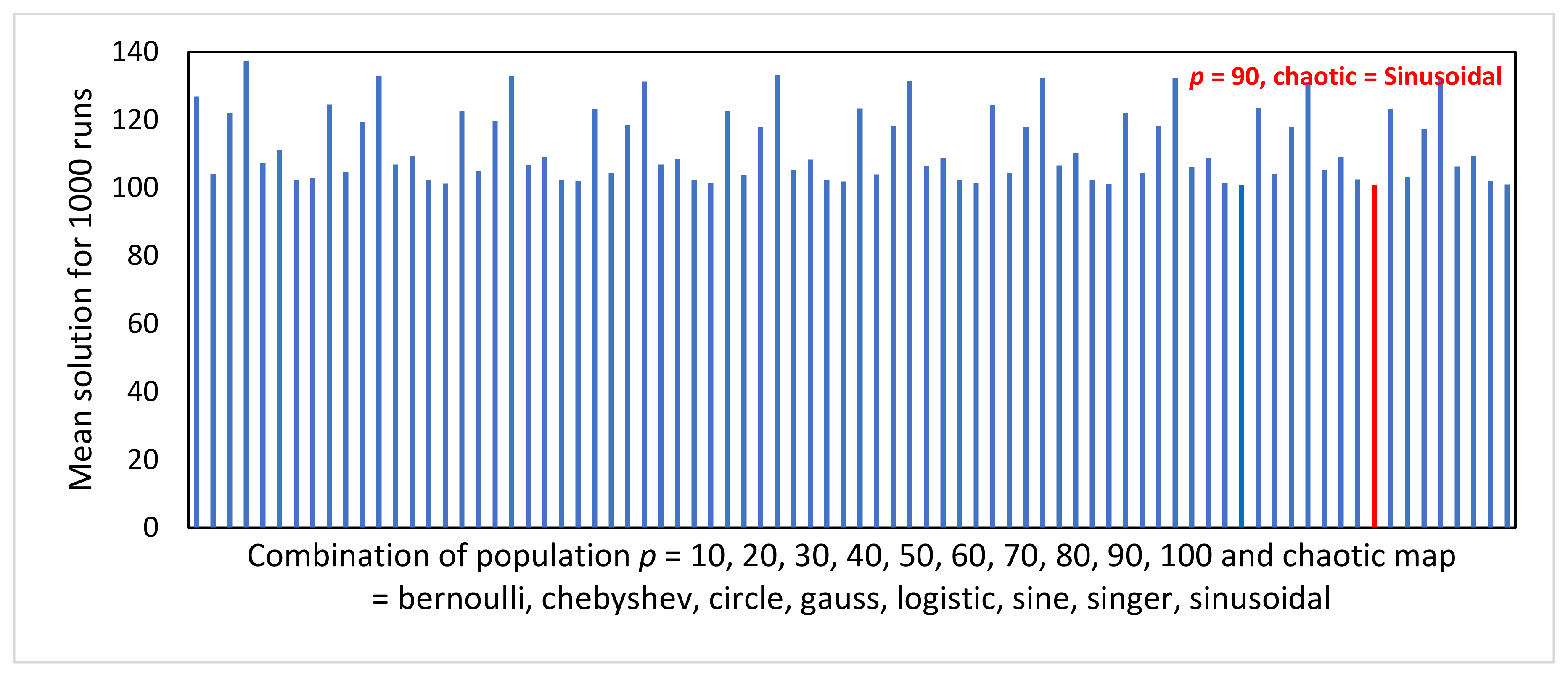
Finally, Figure 4 illustrates the experimental results for the problem of searching for a minimum solution using the COCOMO estimation method. The vertical axis shows all results from eighty experiments. It can be seen that a large population p (90) means the MUCPSO produces a good solution. In contrast, the smaller the p, the worse the solution. Hence, the combination of large p and Sinusoidal as the chaotic function is recommended. The optimum combination is reached for p = 90 and chaotic = Sinusoidal.

6.2. Parameter Settings

Based on previous research in [23,24,47,64], the best population size for each algorithm has been defined. However, due to the difference of function between software effort estimation methods, we conducted ten experiments with p = 10, 20, …, 100 to find the optimum p for each algorithm based on the Friedman Mean Rank (FMR).

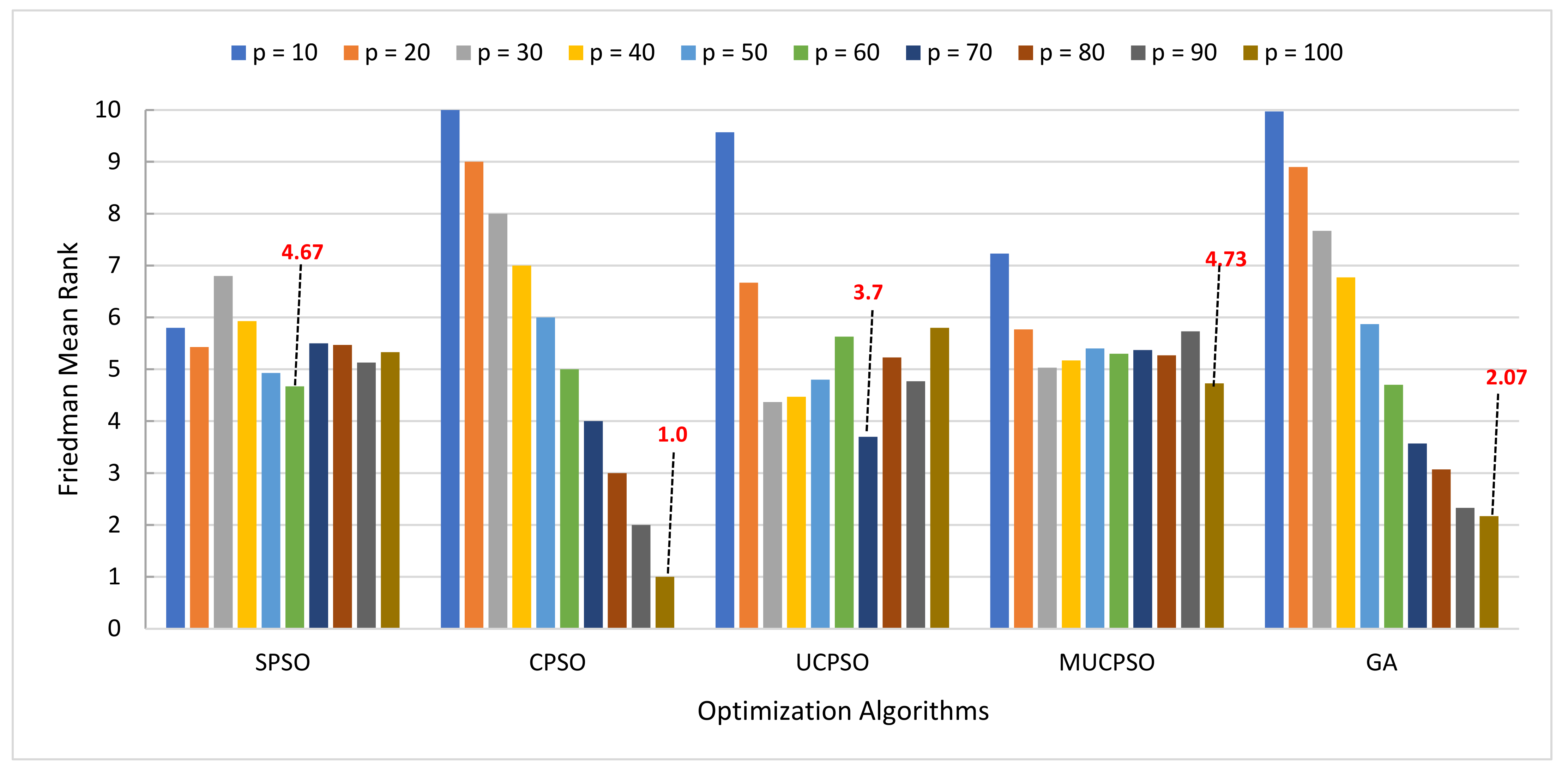
Figure 5 illustrates the experimental results for the COCOMO estimation method. The behavior of p is quite similar for CPSO, MUCPSO, and GA. The larger the p, the better the rank. The optimum value is reached using p = 100 for the three algorithms. Meanwhile, p gives a different effect for SPSO and UCPSO that achieves the optimum value through p = 60 and 70, respectively.

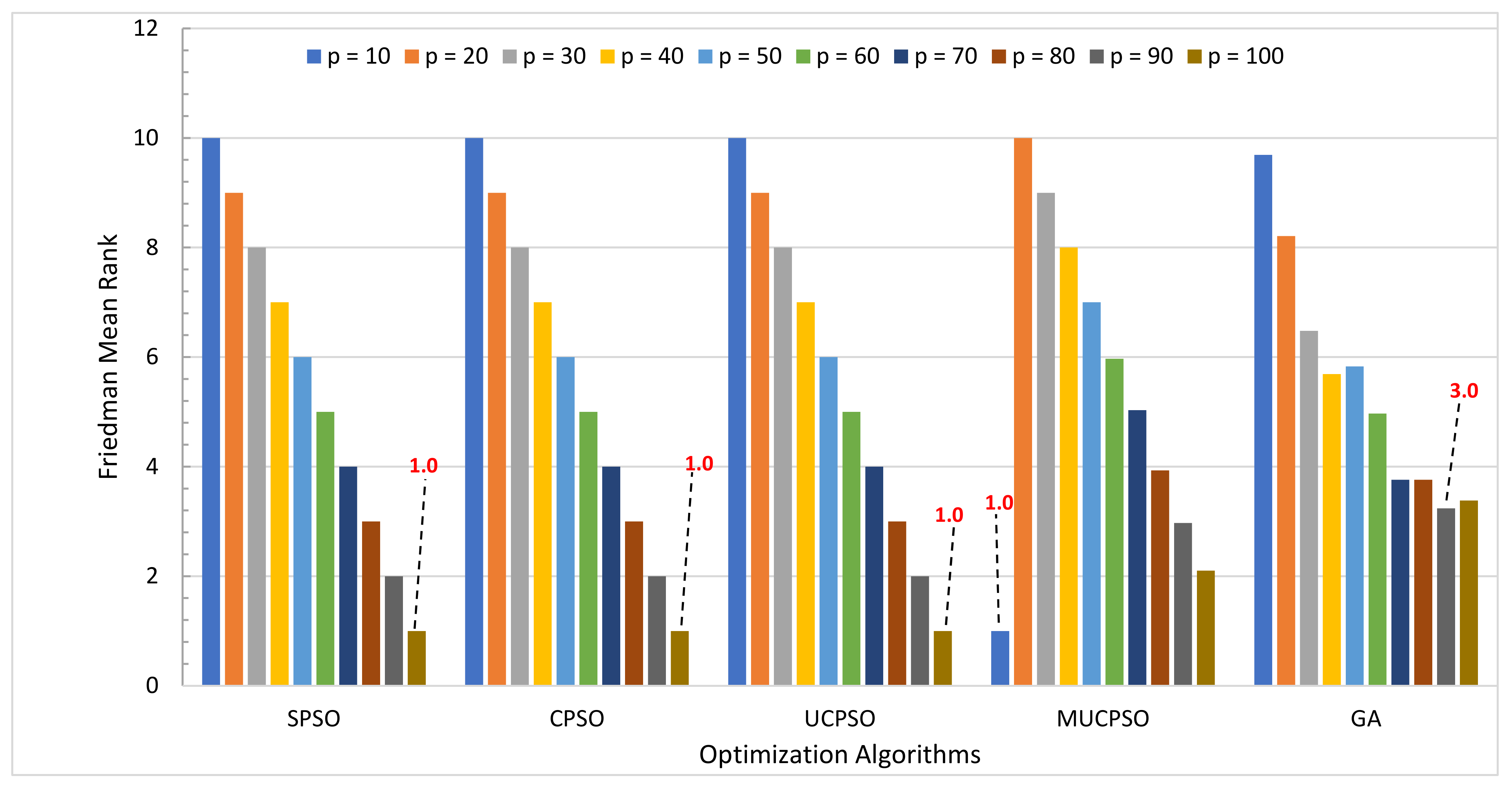
Next, Figure 6 illustrates the experiment results for the UCP estimation method. The behavior of p is similar for SPSO, CPSO, and UCPSO. The larger the p, the better the rank. The optimum value is reached on p = 100 for the three algorithms. Meanwhile, the behavior of p provides a different effect for MUCPSO and GA that achieves the optimum value via p = 10 and 90, respectively.

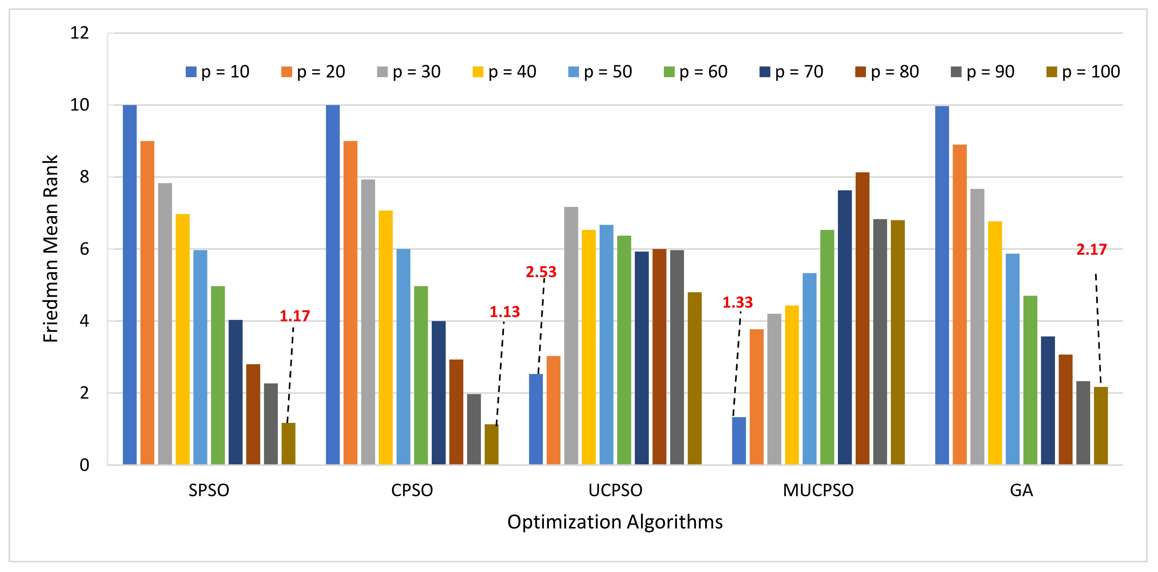
Finally, Figure 7 illustrates the experimental results for the Agile estimation method. The behavior of p is similar for SPSO, CPSO, and GA. The larger the p, the better the rank. The optimum value is reached using p = 100 for the three algorithms. Meanwhile, the behavior of p also provides similar effect for UCPSO and MUCPSO that achieves the optimum value through p = 10.

The parameter settings for MUCPSO and other benchmark algorithms are listed in

Table 4. Parameter settings.

Algorithms	Parameter Settings	Ref.
SPSO	$\omega :0.9~0.4, c_1=c_2=2, r_1=r_2=\mathrm{rand} \left[0,1\right]$, $p_{\mathrm{agile}}=100, p_{\mathrm{cocomo}}=60, p_{\mathrm{UCP}}=100$	[64]
CPSO	$p=40, \omega :0.9~0.4, c_1=c_2=1.5, r_1=\mathrm{Singer}, r_2=\mathrm{Sine}$, $p_{\mathrm{agile}}=100, p_{\mathrm{cocomo}}=100, p_{\mathrm{UCP}}=100$	[24]
GA	$\mathrm{crossover} \mathrm{rate}:0.8,$$\mathrm{mutation} \mathrm{rate}\text{:} 1/\mathrm{popSize}, \mathrm{elitism} \mathrm{selection}, p_{\mathrm{agile}}=100, p_{\mathrm{cocomo}}=100, p_{\mathrm{UCP}}=90$	[25]
UCPSO	$\omega :0.9~0.4, c_1=c_2=2, r_1=r_2=\mathrm{rand}\left[0,1\right]$$, p_{\mathrm{agile}}=10, p_{\mathrm{cocomo}}=70, p_{\mathrm{UCP}}=100$, cosine map	[23]
MUCPSO	$\omega :0.9~0.4, c_1=c_2=2, r_1=r_2=\mathrm{chaotic}$$, p_{\mathrm{agile}}=10, p_{\mathrm{cocomo}}=100, p_{\mathrm{UCP}}=10$	Presented

. Parameters c₁ and c₂ are set to integer two since it, on average, sets the weights for “social” and “cognition” to 1 [14,64]. The stochastic parameters r₁ and r₁ are two random functions in the range [0,1] [64]. The parameters are introduced in SPSO, and UCPSO, while CPSO and MUCPSO use the chaotic map function as their stochastic parameters.

6.3. Investigation on Three Estimation Methods

The proposed MUCPSO algorithm is examined and compared with four other algorithms, as follows: SPSO, CPSO, GA, and UCPSO to search the optimum solutions to the UCP, COCOMO, and Agile estimation method as formulated in Equation (10) to Equation (25). For each estimation method, the maximum particles size is set to 2500, with 30 runs to reduce the coincidence. The random seeds of the 30 initial populations (for each estimation method) are the same to obtain fairness. The evolution is illustrated using the step sizes of 40 to obtain fairness. Thus, all the algorithms show the same generations from 20 to 980.

Table 5. Comparison of SPSO, CPSO, GA, UCPSO, and MUCPSO for 3 software estimation methods.

Method	Metric	SPSO	CPSO	GA	UCPSO	MUCPSO
UCP	Best	1009.26	1009.31	1071.29	1009.46	1009.14
	Worst	1011.25	1011.51	1162.35	1010.16	1010.28
	Mean	1010.21	1010.34	1123.26	1009.9	1009.81
	STD	0.47	0.56	27.64	0.18	0.32
COCOMO	Best	21.06	24.39	61.94	28.56	25.58
	Worst	271.68	301.14	642.35	49.4	40.32
	Mean	63.97	68.92	183.24	40.89	34.43
	STD	53.7	60.27	144.22	5.32	3.18
Agile	Best	13.466	13.466	16.597	13.463	13.461
	Worst	13.587	13.570	24.883	13.537	13.493
	Mean	13.498	13.49	21.643	13.488	13.475
	STD	0.029	0.021	1.974	0.014	0.007
	FMR	2.87	3.13	4.07	3.44	1.67
	Rank	2	3	5	4	1

illustrates the examination results based on the following four metrics: best solution, worst solution, mean solution, and standard deviation (STD) as explained further in the following passages.

The best solution for UCP estimation is yielded by MUCPSO, whereas the highest worst and mean solution metric is obtained using UCPSO, and MUCPSO, respectively. If we compare the two lower standard deviation values between MUCPSO (0.32) and UCPSO (0.18), we can observe that the deviation value is slightly different. Hence, we can conclude that UCPSO and MUCPSO has the smallest and smaller amount of variation, respectively. In other words, the mean for MUCPSO is less reliable than the mean for MUCPSO.

The lowest best and mean solution for COCOMO estimation is yielded by SPSO, MUCPSO, respectively, whereas the highest worst solution is yielded by MUCPSO. Although SPSO has the lowest best solution, however, due to the lowest mean and standard deviation is yielded by MUCPSO compared with four other algorithms, we can conclude that MUCPSO has the smallest amount of variation and most reliable for the mean value.

The lowest solution value for Agile estimation is yielded by MUCPSO in terms of the best and mean solution. For the highest worst solution is also yielded by MUCPSO. This result is supported by its lowest standard deviation value (0.007), indicating that MUCPSO has the smallest amount of variation which means that the data points are most concentrated around the reliable mean solution. Furthermore, based on the Friedman mean rank (FMR), we can observe that MUCPSO yielded the first rank, followed by SPSO, CPSO, UCPSO, and GA.

The Wilcoxon rank-sum test illustrated in

Table 6. The p-value of Wilcoxon rank sum test (WRST) for 3 estimation benchmark methods.

Method	MUCPSO vs. SPSO	MUCPSO vs. CPSO	MUCPSO vs. GA	MUCPSO vs. UCPSO
UCP	0.000716	0.000148	0.000002	0.271155
COCOMO	0.000241	0.000049	0.000002	0.000034
Agile	0.000097	0.000283	0.000002	0.000616

confirms that MUCPSO is significantly better than all the competitor algorithms for the three estimation benchmark methods. All the p-values are lower than the significance level of 0.05, except the UCP estimation where MUCPSO is worse than UCPSO with a p-value of greater than 0.05. However, since the proposed method has 11 better results (91.67%) out of 12 significant results, we can conclude that the proposed method is better than most of the benchmark algorithms in almost all the estimation methods.

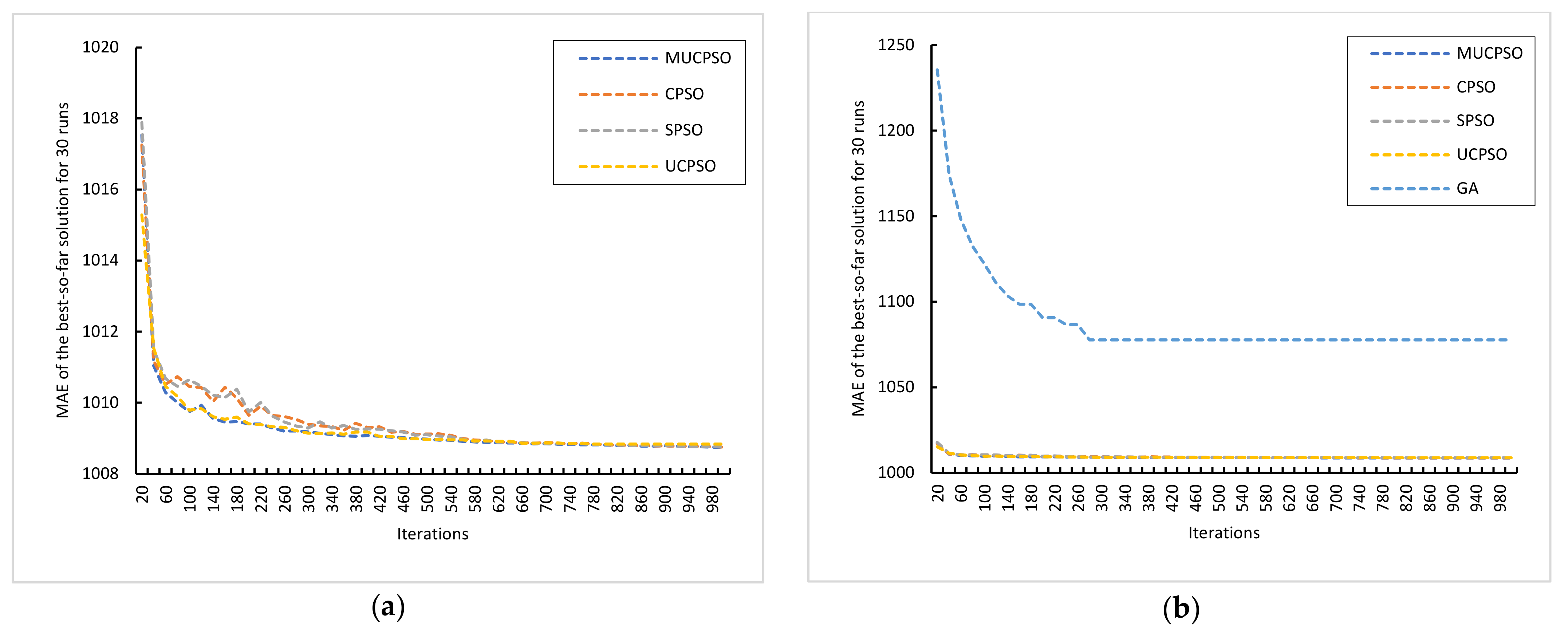
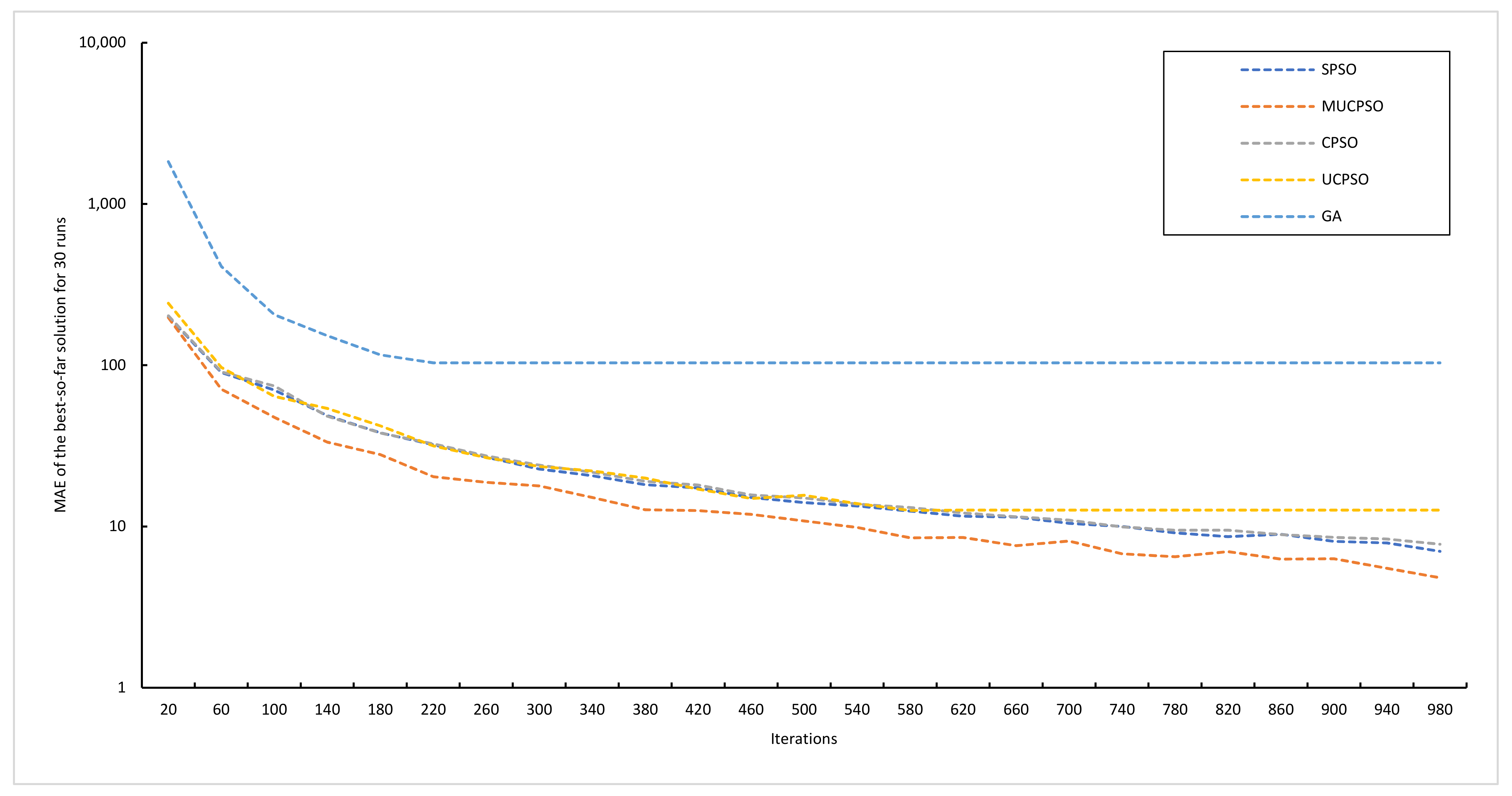
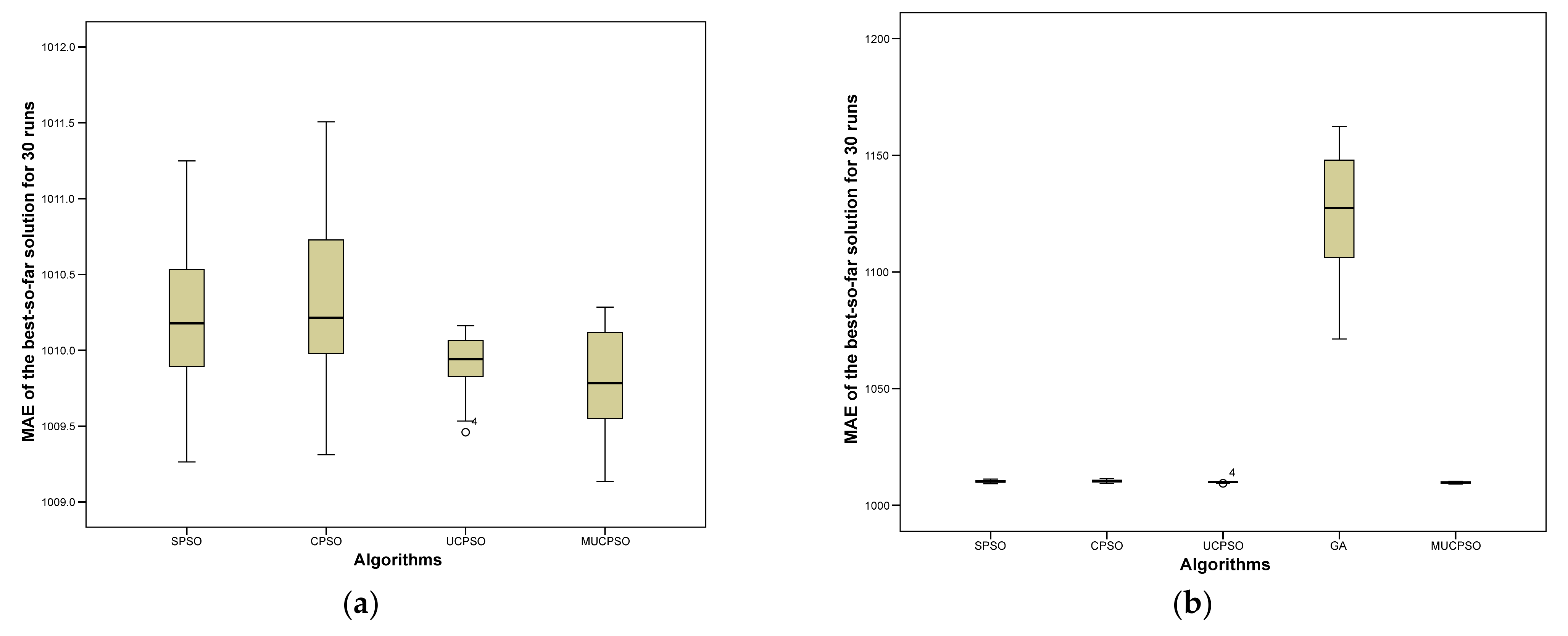
Furthermore, we discussed the detailed investigations of the convergence analysis of MUCPSO and its competitors. For each estimation method benchmark, the maximum number of particles is set to 2500 with 30 runs. Figure 8a illustrates the evolutionary processes of four algorithms (SPSO, CPSO, UCPSO, and MUCPSO) until they converge with the optimum solution for the UCP estimation method. Figure 8b illustrates the evolutionary process of all of the algorithms until convergence with the optimum solution. In this benchmark, MUCPSO converges to a much better solution than the other algorithms. Impressively, MUCPSO evolves at the greatest speed in the initial generations and finally provides the best mean solution of 1009.81.

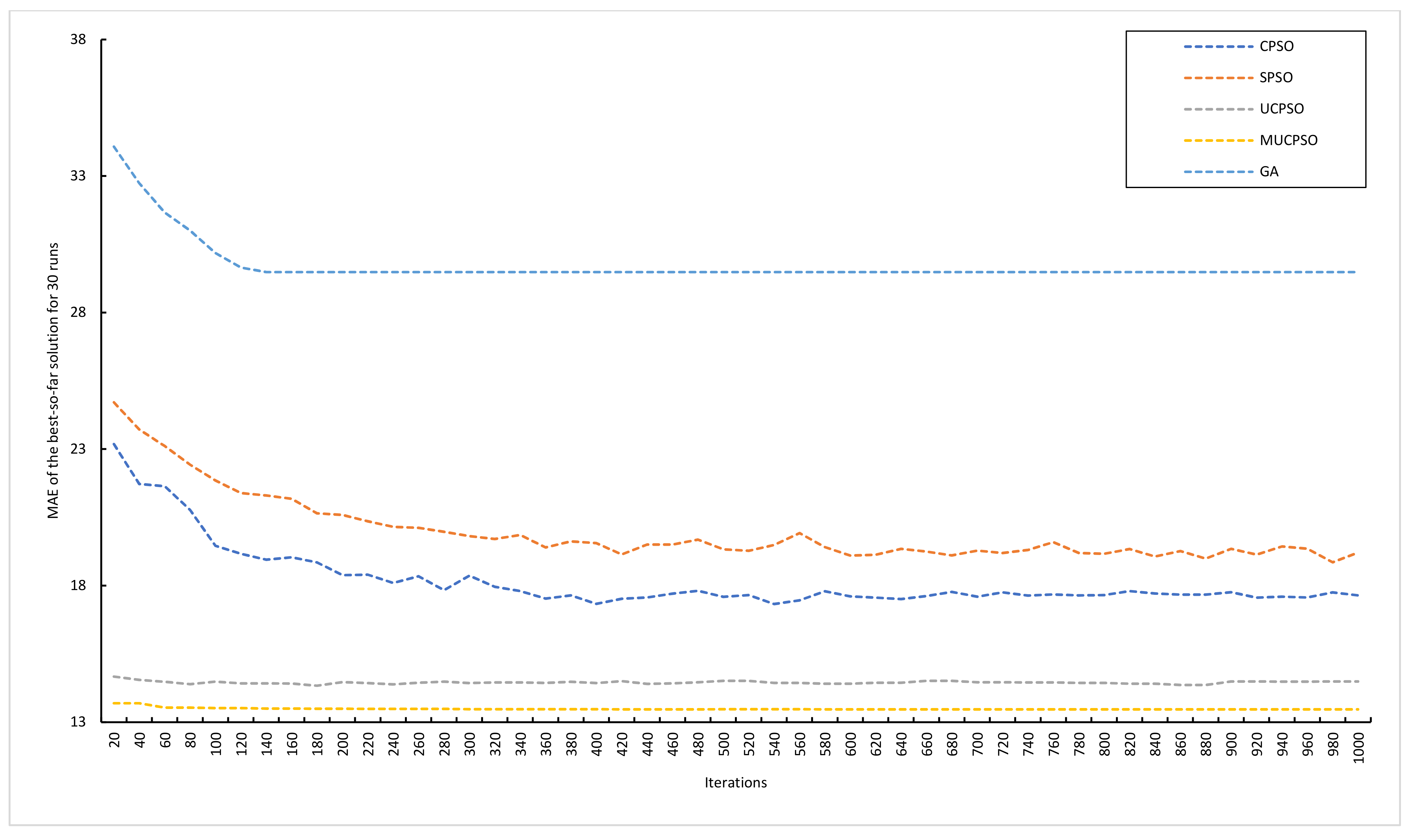
Next, the convergence analysis is provided for the COCOMO estimation method benchmark. Figure 9 illustrates the evolutionary processes of all algorithms until convergence with the optimum solution. In this benchmark, MUCPSO converges to a much better solution than the SPSO, CPSO, GA, and UCPSO algorithm. MUCPSO demonstrates and impressive convergence from the beginning to the end of generation.

Finally, Figure 10 illustrates the evolutionary processes of all algorithms until convergence with the optimum solution for the Agile estimation method. In this benchmark, MUCPSO converges stably to the better solution than the other algorithm. From the beginning of generation, MUCPSO is able to compete with four other algorithms and finally provides the best mean solution of 13.475.

Beside the convergence analysis, we further explore the diversity analysis of the best solution for the benchmark algorithm using three effort estimation methods. Figure 11 depicts the diversity analysis for UCP estimation. Figure 11a depicts the diversity analysis between four algorithms (SPSO, CPSO, UCPSO, and MUCPSO), excluding GA, to demonstrate a clearer center and the spreads of each result. Based on Figure 11a, we can observe that the median for MUCPSO is smaller compared with SPSO, CPSO and UCPSO. However, the spread of MUCPSO is quite large compared with UCPSO. In Figure 11b, we compare all benchmark algorithms, including GA. We are able to observe that the difference between GA and the aforementioned algorithms is quite large.

Next, we analyze the diversity of COCOMO estimation. Figure 12 shows that the median of SPSO, CPSO, UCPSO, and MUCPSO is quite similar. However, based on the interquartile box, we can observe that MUCPSO has the smallest shape compared with other algorithms. This shape indicates that MUCPSO has the lowest spread.

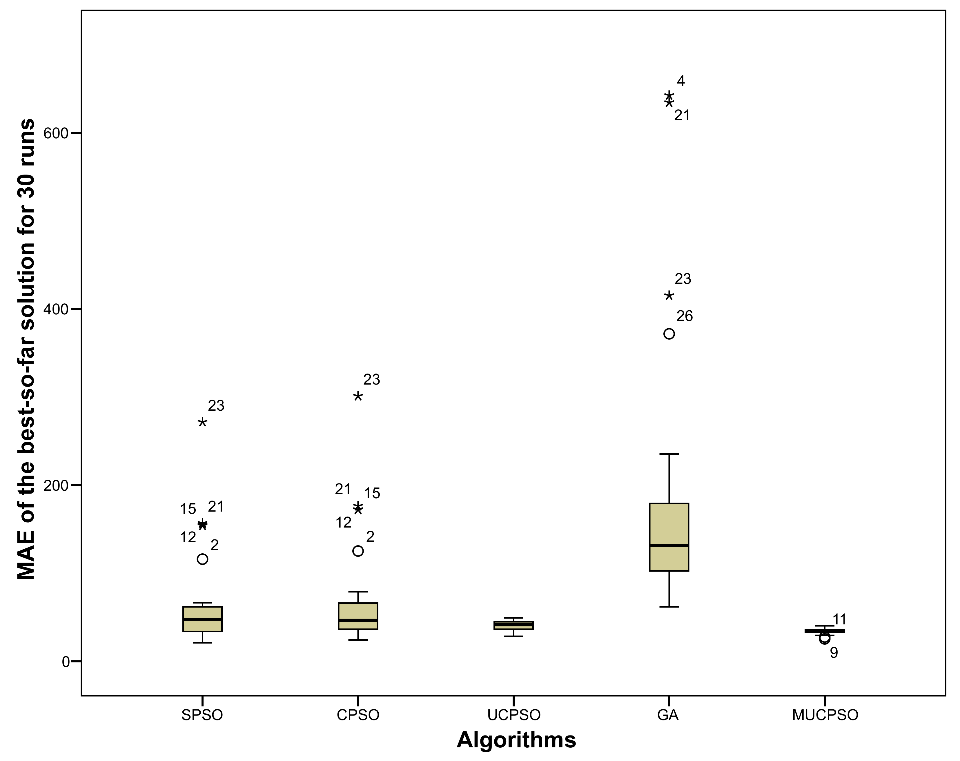
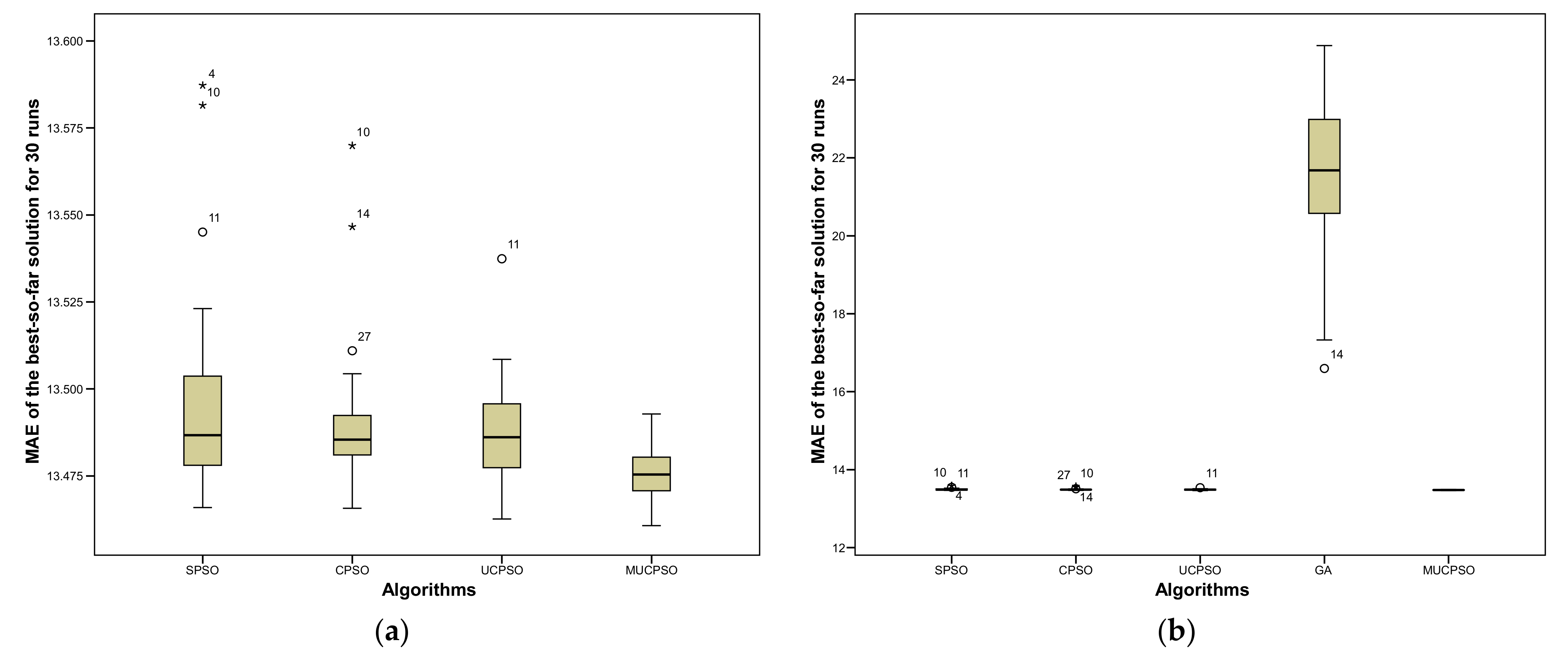
Finally, Figure 13 describe the diversity analysis of Agile estimation. Similar to Figure 11, we split the results into two parts, presented as Figure 13a,b. Due to the large difference observed when including GA in the group of boxplots, we provide clearer results by excluding GA in Figure 13a. Based on the boxplots in Figure 13a we observe that MUCPSO has the lowest median, whereas the rest (SPSO, CPSO, and UCPSO) are quite similar. Furthermore, the interquartile of MUCPSO shows the smallest shape, indicating that the proposed method has the lowest spread. Almost identical with Figure 11b, when GA is included, the difference of results is found to be very large, and a comparison of the rest of the algorithms proves quite difficult.

7. Conclusions and Future Work

Particle swarm optimization (PSO) is widely used for different applications in software engineering domains such as in the next release problem, risk factor prioritization, and software-effort estimation. There are numerous variants of the PSO algorithm proposed to improve its performance. However, PSO still suffers from two primary shortcomings—premature convergence and easy trap in local optima. This study proposes modified chaotic particles swarm optimization with uniform initialized particles (MUCPSO). This algorithm works well based on the following three schemes: uniform initialization, chaotic inertia mapping, and a stochastic personal learning strategy. Uniform initialization is applied to ensure the diversity of the initialized particle, while chaotic inertia weight plays a role in maintaining the balance between the exploration and exploitation phases, and personal learning strategy helps to enhance the global and local search to avoid trap in local optima. The evaluation of three estimation method benchmarks shows that it significantly outperforms all the competitors, including SPSO, CPSO, GA, and UCPSO, where it reaches the Friedman mean rank of 1.67, with p-values of the Wilcoxon rank-sum test of less than 0.05 for most of the benchmarks. Detailed investigations prove that all the proposed schemes work well in their designed and mean MUCPSO can effectively control the exploration and exploitation balance. The proposed schemes mean MUCPSO is able to handle most of the various estimation method benchmark functions.

Several directions for future studies are suggested. First, due to the slightly worse result yielded by MUCPSO compared with CPSO in the COCOMO estimation method benchmark, in future, further studies will be conducted by increasing the generation number. This scenario is important to provide more room to explore MUCPSO and the probability of the best result that can be achieved. Second, the addition of further data and another variants of the estimation method should be employed to enhance the performance of the MUCPSO algorithm.

References

1. Choetkiertikul, M.; Dam, H.K.; Tran, T.; Ghose, A.; Grundy, J. Predicting Delivery Capability in Iterative Software Development. IEEE Trans. Softw. Eng. 2018, 44, 551–573. Available online: https://ieeexplore.ieee.org/abstract/document/7898472 (accessed on 11 March 2019). [CrossRef]
2. Kaur, A.; Kaur, K. A COSMIC function points based test effort estimation model for mobile applications. J. King Saud. Univ. Comput. Inf. Sci. 2019, in press. Available online: https://linkinghub.elsevier.com/retrieve/pii/S131915781831317X (accessed on 12 March 2019).
3. Rak, K.; Car, Ž.; Lovrek, I. Effort estimation model for software development projects based on use case reuse. J. Softw. Evol. Process 2019, 31, e2119. Available online: http://doi.wiley.com/10.1002/smr.2119 (accessed on 4 November 2018). [CrossRef]
4. Boehm, B.; Abts, C.; Chulani, S. Software development cost estimation approaches—A survey. Ann. Softw. Eng. 2000, 10, 177–205. [Google Scholar] [CrossRef]
5. Angeline, P.J. Using selection to improve particle swarm optimization. In Proceedings of the 1998 IEEE International Conference on Evolutionary Computation Proceedings IEEE World Congress on Computational Intelligence (Cat No98TH8360), Anchorage, AK, USA, 4–9 May 1998; IEEE: Anchorage, AK, USA, 2002; pp. 84–89. [Google Scholar]
6. Chen, Y.; Li, L.; Xiao, J.; Yang, Y.; Liang, J.; Li, T. Engineering Applications of Artificial Intelligence Particle swarm optimizer with crossover operation. Eng. Appl. Artif. Intell. 2018, 70, 159–169. [Google Scholar] [CrossRef]
7. Dong, W.; Kang, L.; Zhang, W. Opposition-based particle swarm optimization with adaptive mutation strategy. Soft Comput. 2017, 21, 5081–5090. [Google Scholar] [CrossRef]
8. Jindal, V.; Bedi, P. An improved hybrid ant particle optimization (IHAPO) algorithm for reducing travel time in VANETs. Appl. Soft Comput. 2018, 64, 526–535. [Google Scholar] [CrossRef]
9. Wang, S.; Li, Y.; Yang, H. Self-adaptive mutation differential evolution algorithm based on particle swarm optimization. Appl. Soft Comput. 2019, 81, 1–22. [Google Scholar] [CrossRef]
10. Nakano, S.; Ishigame, A.; Yasuda, K. Consideration of Particle Swarm Optimization combined with tabu search. Electr. Eng. Jpn. 2010, 172, 31–37. [Google Scholar] [CrossRef]
11. El-Abd, M. Testing a Particle Swarm Optimization and Artificial Bee Colony Hybrid algorithm on the CEC13 benchmarks. In Proceedings of the 2013 IEEE Congress on Evolutionary Computation, Cancun, Mexico, 20–23 June 2013; IEEE: Cancun, Mexico, 2013; pp. 2215–2220. [Google Scholar]
12. Aydilek, I.B. A hybrid firefly and particle swarm optimization algorithm for computationally expensive numerical problems. Appl. Soft Comput. 2018, 66, 232–249. [Google Scholar] [CrossRef]
13. Nagra, A.A.; Fei, H.; Ling, Q.H.; Mehta, S. An Improved Hybrid Method Combining Gravitational Search Algorithm With Dynamic Multi Swarm Particle Swarm Optimization. IEEE Access 2019, 7, 50388–50399. [Google Scholar] [CrossRef]
14. Kennedy, J.; Eberhart, R. Particle swarm optimization. In Proceedings of the ICNN’95—International Conference on Neural Networks, Perth, WA, Australia, 27 November–1 December; IEEE: Perth, WA, Australia, 1995; pp. 1942–1948. Available online: http://ieeexplore.ieee.org/document/488968/ (accessed on 6 January 2020).
15. Benala, T.R.; Mall, R. DABE: Differential evolution in analogy-based software development effort estimation. Swarm Evol. Comput. 2018, 38, 158–172. [Google Scholar] [CrossRef]
16. Brezočnik, L.; Fister, I.; Podgorelec, V. Solving Agile Software Development Problems with Swarm Intelligence Algorithms. In Lecture Notes in Networks and Systems; Karabegovi, E., Ed.; Springer: Cham, Switzerland; Sarajevo, Bosnia and Herzegovina, 2020; pp. 298–309. Available online: http://link.springer.com/10.1007/978-3-030-18072-0_35 (accessed on 12 January 2021).
17. Peng, Y.; Peng, X.; Liu, Z. Statistic Analysis on Parameter Efficiency of Particle Swarm Optimization. Acta Electron. Sin. 2004, 32, 209–2013. [Google Scholar]
18. Agrawal, A.; Tripathi, S. Particle swarm optimization with probabilistic inertia weight. In Advances in Intelligent Systems and Computing; Yadav, N., Yadav, A., Bansal, J.C., Deep, K., Kim, J.H., Eds.; Springer Singapore: Gurgaon, India, 2019; pp. 239–248. [Google Scholar]
19. Ratnaweera, A.; Halgamuge, S.K.; Watson, H.C. Self-Organizing Hierarchical Particle Swarm Acceleration Coefficients. IEEE Trans. Evol. Comput. 2004, 8, 240–255. [Google Scholar] [CrossRef]
20. Lin, A.; Sun, W.; Yu, H.; Wu, G.; Tang, H. Global genetic learning particle swarm optimization with diversity enhancement by ring topology. Swarm Evol. Comput. 2019, 44, 571–583. [Google Scholar] [CrossRef]
21. Vafashoar, R.; Meybodi, M.R. Cellular learning automata based bare bones PSO with maximum likelihood rotated mutations. Swarm Evol. Comput. 2019, 44, 680–694. [Google Scholar] [CrossRef]
22. Wang, Y.; Liu, H.; Yu, Z.; Tu, L. An improved artificial neural network based on human-behaviour particle swarm optimization and cellular automata. Expert Syst. Appl. 2020, 140, 112862. [Google Scholar] [CrossRef]
23. Zhang, J.; Sheng, J.; Lu, J.; Shen, L. UCPSO: A Uniform Initialized Particle Swarm Optimization Algorithm with Cosine Inertia Weight. Comput. Intell. Neurosci. 2021, 2021, 8819333. Available online: https://www.hindawi.com/journals/cin/2021/8819333/ (accessed on 9 May 2021). [CrossRef] [PubMed]
24. Tharwat, A.; Elhoseny, M.; Hassanien, A.E.; Gabel, T.; Kumar, A. Intelligent Bézier curve-based path planning model using Chaotic Particle Swarm Optimization algorithm. Clust. Comput. 2019, 22, 4745–4766. [Google Scholar] [CrossRef]
25. Holland, J.H. Adaptation in Natural and Artificial Systems; MIT Press: London, UK, 1992. [Google Scholar]
26. Tian, D.; Zhao, X.; Shi, Z. DMPSO: Diversity-Guided Multi-Mutation Particle Swarm Optimizer. IEEE Access 2019, 7, 124008–124025. Available online: https://ieeexplore.ieee.org/document/8817908/ (accessed on 11 June 2021). [CrossRef]
27. Singh, M.R.; Mahapatra, S.S. A quantum behaved particle swarm optimization for flexible job shop scheduling. Comput. Ind. Eng. 2016, 93, 36–44. [Google Scholar] [CrossRef]
28. Tian, D. Particle Swarm Optimization with Chaos-based Initialization for Numerical Optimization. Intell. Autom. Soft Comput. 2018, 24, 331–342. [Google Scholar] [CrossRef]
29. Zhang, H.; Xie, J.; Hu, Q.; Shao, L.; Chen, T. A hybrid DPSO with Levy flight for scheduling MIMO radar tasks. Appl. Soft Comput. J 2018, 71, 242–254. [Google Scholar] [CrossRef]
30. Xu, X.; Rong, H.; Trovati, M.; Liptrott, M.; Bessis, N. CS-PSO: Chaotic particle swarm optimization algorithm for solving combinatorial optimization problems. Soft Comput. 2018, 22, 783–795. Available online: http://link.springer.com/10.1007/s00500-016-2383-8 (accessed on 10 June 2021). [CrossRef] [Green Version]
31. Abdullah, H. An Improvement in LQR Controller Design based on Modified Chaotic Particle Swarm Optimization and Model Order Reduction. Int. J. Intell. Eng. Syst. 2021, 14, 157–168. Available online: http://www.inass.org/2021/2021022816.pdf (accessed on 14 June 2021). [CrossRef]
32. Ma, Z.; Yuan, X.; Han, S.; Sun, D.; Ma, Y. Improved Chaotic Particle Swarm Optimization Algorithm with More Symmetric Distribution for Numerical Function Optimization. Symmetry 2019, 11, 876. Available online: https://www.mdpi.com/2073-8994/11/7/876 (accessed on 14 June 2021). [CrossRef] [Green Version]
33. Rahnamayan, S.; Tizhoosh, H.R.; Salama, M.M.A. Opposition-Based Differential Evolution Algorithms. In Proceedings of the 2006 IEEE International Conference on Evolutionary Computation Vancouver, Vancouver, BC, Canada, 16–21 July 2006; IEEE: Vancouver, BC, Canada, 2006; pp. 2010–2017. Available online: http://ieeexplore.ieee.org/document/1688554/ (accessed on 11 June 2021).
34. Wang, H.; Wu, Z.; Rahnamayan, S. Enhanced opposition-based differential evolution for solving high-dimensional continuous optimization problems. Soft Comput. 2011, 15, 2127–2140. Available online: http://link.springer.com/10.1007/s00500-010-0642-7 (accessed on 10 June 2021). [CrossRef]
35. Rehman, A.U.; Islam, A.; Belhaouari, S.B. Multi-Cluster Jumping Particle Swarm Optimization for Fast Convergence. IEEE Access 2020, 8, 189382–189394. Available online: https://ieeexplore.ieee.org/document/9223747/ (accessed on 10 June 2021). [CrossRef]
36. Rauf, H.T.; Shoaib, U.; Lali, M.I.; Alhaisoni, M.; Irfan, M.N.; Khan, M.A. Particle Swarm Optimization With Probability Sequence for Global Optimization. IEEE Access 2020, 8, 110535–110549. Available online: https://ieeexplore.ieee.org/document/9117125/ (accessed on 10 June 2021). [CrossRef]
37. Arif, M.; Chen, J.; Wang, G.; Rauf, H.T. Cognitive population initialization for swarm intelligence and evolutionary computing. J. Ambient. Intell. Humaniz. Comput. 2021, 1–14. [Google Scholar] [CrossRef]
38. Eberhart, R.; Shi, Y. Tracking and optimizing dynamic systems with particle swarms. In Proceedings of the 2001 Congress on Evolutionary Computation (IEEE Cat No01TH8546), Seoul, Korea, 27–30 May 2001; IEEE: Seoul, Korea, 2001; pp. 94–100. Available online: http://ieeexplore.ieee.org/document/934376/ (accessed on 14 June 2021).
39. Cheng, R.; Jin, Y. A social learning particle swarm optimization algorithm for scalable optimization. Inf. Sci. 2015, 291, 43–60. [Google Scholar] [CrossRef]
40. Zhang, X.; Wang, X.; Kang, Q.; Cheng, J. Differential mutation and novel social learning particle swarm optimization algorithm. Inf. Sci. 2019, 480, 109–129. [Google Scholar] [CrossRef]
41. Sedighizadeh, D.; Masehian, E.; Sedighizadeh, M.; Akbaripour, H. GEPSO: A new generalized particle swarm optimization algorithm. Math. Comput. Simul. 2021, 179, 194–212. [Google Scholar] [CrossRef]
42. Chen, H.; Wang, W.; Chen, X.; Qiu, L. Multi-objective reservoir operation using particle swarm optimization with adaptive random inertia weights. Water Sci. Eng. 2020, 13, 136–144. [Google Scholar] [CrossRef]
43. Nagra, A.A.; Han, F.; Ling, Q.H. An improved hybrid self-inertia weight adaptive particle swarm optimization algorithm with local search. Eng. Optim. 2019, 51, 1115–1132. [Google Scholar] [CrossRef]
44. Shi, Y.; Eberhart, R.C. Fuzzy adaptive particle swarm optimization. In Proceedings of the 2001 Congress on Evolutionary Computation (IEEE Cat No01TH8546), Seoul, Korea, 27–30 May 2001; IEEE: Seoul, Korea; pp. 101–106. Available online: http://ieeexplore.ieee.org/document/934377/ (accessed on 14 June 2021).
45. Chen, K.; Zhou, F.; Liu, A. Chaotic dynamic weight particle swarm optimization for numerical function optimization. Knowl. Based Syst. 2018, 139, 23–40. Available online: https://linkinghub.elsevier.com/retrieve/pii/S0950705117304719 (accessed on 14 June 2021). [CrossRef]
46. Koyuncu, H. GM-CPSO: A New Viewpoint to Chaotic Particle Swarm Optimization via Gauss Map. Neural. Process. Lett. 2020, 52, 241–266. [Google Scholar] [CrossRef]
47. Liu, H.; Zhang, X.W.; Tu, L.P. A modified particle swarm optimization using adaptive strategy. Expert. Syst. Appl. 2020, 152, 113353. [Google Scholar] [CrossRef]
48. Xu, G.; Cui, Q.; Shi, X.; Ge, H.; Zhan, Z.-H.; Lee, H.P.; Liang, Y.; Tai, R.; Wu, C. Particle swarm optimization based on dimensional learning strategy. Swarm Evol. Comput. 2019, 45, 33–51. [Google Scholar] [CrossRef]
49. Ye, W.; Feng, W.; Fan, S. A novel multi-swarm particle swarm optimization with dynamic learning strategy. Appl. Soft Comput. 2017, 61, 832–843. [Google Scholar] [CrossRef]
50. Wang, F.; Zhang, H.; Li, K.; Lin, Z.; Yang, J.; Shen, X.-L. A hybrid particle swarm optimization algorithm using adaptive learning strategy. Inf. Sci. 2018, 436–437, 162–177. [Google Scholar] [CrossRef]
51. Lin, A.; Sun, W.; Yu, H.; Wu, G.; Tang, H. Adaptive comprehensive learning particle swarm optimization with cooperative archive. Appl. Soft Comput. 2019, 77, 533–546. [Google Scholar] [CrossRef]
52. Zhou, S.; Sha, L.; Zhu, S.; Wang, L. Adaptive hierarchical update particle swarm optimization algorithm with a multi-choice comprehensive learning strategy. Appl. Intell. 2021, 1–25. Available online: https://link.springer.com/10.1007/s10489-021-02413-3 (accessed on 14 June 2021). [CrossRef]
53. Silhavy, R. Use Case Points Benchmark Dataset v1; Mendeley Data: Zlin, Czech Republic, 2017; Available online: https://data.mendeley.com/datasets/2rfkjhx3cn/1 (accessed on 23 December 2019).
54. Menzies, T. Nasa93 [Data set]; Zenodo: Raleigh, NC, USA, 2008; Available online: https://zenodo.org/record/268419#.YOk5FDPitEY (accessed on 11 August 2018).
55. Zia, Z.; Tipu, S.K.; Zia, S. An Effort Estimation Taxonomy for Agile Software Development. Adv. Comput. Sci. Appl. 2012, 2, 314–324. Available online: https://www.worldscientific.com/doi/abs/10.1142/S0218194017500243 (accessed on 9 July 2021).
56. Karner, G. Resource Estimation for Objectory Projects; University of Linköping: Linköping, Sweden, 1993. [Google Scholar]
57. Hariyanto, M.; Wahono, R.S. Estimasi Proyek Pengembangan Perangkat Lunak Dengan Fuzzy Use Case Points. J. Softw. Eng. 2015, 1, 54–63. [Google Scholar]
58. Capretz, L.F. Enhancing Use Case Points Estimation Method Using Soft Computing Techniques. J. Glob. Res. Comp. Science. 2010, 1, 4. [Google Scholar]
59. Sholiq Subriadi, A.P.; Muqtadiroh, F.A.; Dewi, R.S. A model of owner estimate cost for software development project in Indonesia. J. Softw. Evol. Process 2019, 31, 31. [Google Scholar]
60. Subriadi Pribadi, A.; Ningrum, P.A. Critical Review of the Effort Rate Value in Use Case Point Method for Estimating Software Development Effort. J. Appl. Inf. Technol. 2014, 59, 735–744. [Google Scholar]
61. Azzeh, M.; Nassif, A.B. Project productivity evaluation in early software effort estimation. J. Softw. Evol. Process 2018, 30, 735–744. Available online: https://onlinelibrary.wiley.com/doi/abs/10.1002/smr.2110 (accessed on 17 March 2019). [CrossRef]
62. Boehm, B.; Clark, B.; Horowitz, E.; Westland, C.; Madachy, R.; Selby, R. Cost models for future software life cycle processes: COCOMO 2.0. Ann. Softw. Eng. 1995, 1, 57–94. Available online: http://link.springer.com/10.1007/BF02249046 (accessed on 22 June 2015). [CrossRef]
63. Suyanto, S.; Wibowo, A.T.; Faraby SAl Saadah, S.; Rismala, R. Evolutionary Rao algorithm. J. Comput. Sci. 2021, 53, 101368. [Google Scholar] [CrossRef]
64. Shi, Y.; Eberhart, R. A modified particle swarm optimizer. In Proceedings of the 1998 IEEE International Conference on Evolutionary Computation Proceedings IEEE World Congress on Computational Intelligence (Cat No98TH8360), Anchorage, AK, USA, 4–9 May 1998; IEEE: Anchorage, AK, USA, 1998; pp. 69–73. Available online: http://ieeexplore.ieee.org/document/699146/ (accessed on 6 January 2020).
Figure 1. Chaotic value distributions during 100 iterations.
Applsci 12 01081 g001
Figure 2. Parameter tuning for Use Case Points estimation model.
Applsci 12 01081 g002
Figure 3. Parameter tuning for Agile estimation model.
Applsci 12 01081 g003
Figure 4. Parameter tuning for COCOMO estimation model.
Applsci 12 01081 g004
Figure 5. Friedman mean rank calculated using 10 different population sizes p for each optimization algorithms in COCOMO estimation method.
Applsci 12 01081 g005
Figure 6. Friedman mean rank calculated using 10 different population sizes p for each optimization algorithms in UCP estimation model.
Applsci 12 01081 g006
Figure 7. Friedman mean rank calculated using 10 different population sizes p for each optimization algorithms in Agile estimation model.
Applsci 12 01081 g007
Figure 8. Convergence analysis for UCP estimation (a) of four algorithms (SPSO, CPSO, UCPSO, and MUCPSO); (b) of all algorithms including GA.
Applsci 12 01081 g008
Figure 9. Convergence analysis for COCOMO.
Applsci 12 01081 g009
Figure 10. Convergence analysis for Agile.
Applsci 12 01081 g010
Figure 11. Best solution diversity analysis for UCP (a) of four algorithms (SPSO, CPSO, UCPSO, MUCPSO); (b) of all algorithms including GA.
Applsci 12 01081 g011
Figure 12. Best solution diversity analysis for COCOMO.
Applsci 12 01081 g012
Figure 13. Best solution diversity analysis for Agile of (a) four algorithms (SPSO, CPSO, UCPSO, MUCPSO); (b) all algorithms including GA.
Applsci 12 01081 g013