Article

Deep Compressed Sensing Generation Model for End-to-End Extreme Observation and Reconstruction

College of Information Engineering, Beijing Institute of Petrochemical Technology, Beijing 102617, China
*
Author to whom correspondence should be addressed.
Appl. Sci. 2022, 12(23), 12176; https://doi.org/10.3390/app122312176
Submission received: 1 November 2022 / Revised: 21 November 2022 / Accepted: 27 November 2022 / Published: 28 November 2022
(This article belongs to the Special Issue AI, Machine Learning and Deep Learning in Signal Processing)

Abstract

:
Data transmission and storage are inseparable from compression technology. Compressed sensing directly undersamples and reconstructs data at a much lower sampling frequency than Nyquist, which reduces redundant sampling. However, the requirement of data sparsity in compressed sensing limits its application. The combination of neural network-based generative models and compressed sensing breaks the limitation of data sparsity. Compressed sensing for extreme observations can reduce costs, but the reconstruction effect of the above methods in extreme observations is blurry. We addressed this problem by proposing an end-to-end observation and reconstruction method based on a deep compressed sensing generative model. Under RIP and S-REC, data can be observed and reconstructed from end to end. In MNIST extreme observation and reconstruction, end-to-end feasibility compared to random input is verified. End-to-end reconstruction accuracy improves by 5.20% over random input and SSIM by 0.2200. In the Fashion_MNIST extreme observation and reconstruction, it is verified that the reconstruction effect of the deconvolution generative model is better than that of the multi-layer perceptron. The end-to-end reconstruction accuracy of the deconvolution generative model is 2.49% higher than that of the multi-layer perceptron generative model, and the SSIM is 0.0532 higher.

1. Introduction

Nowadays, people cannot live without digitalization. In this era of digitalization, the primary problem is the storage and transmission of massive amounts of data. In the early days, the process of digital acquisition of analog signals was inseparable from the traditional Nyquist-Shannon sampling theorem, which points out that the sampling frequency must be more than twice the highest frequency of the original signal in order to completely retain the information in the original signal or accurately reconstruct the original signal [1]. However, in the digital age, where the demand for information is surging, the Nyquist-Shannon sampling theorem causes redundant sampling, even with the rapid development of current computer technology. The sampling rate, storage space, transmission bandwidth, and processing speed for huge amounts of data can consume huge resources, and the ways to solve these problems are pointed toward the compression technology of the signal. In 2006, Candes et al. proposed the theory of Compressed sensing [2] (CS), which is different from traditional Nyquist sampling in that the signal could be sampled at much lower frequencies than Nyquist sampling, resulting in less redundancy in the sampled data and complete reconstruction of the original signal with high probability [3]. Compressed sensing has been applied in many aspects [4]. For example, in wireless communications, channel estimation technology based on compressed sensing has been proposed to improve spectral efficiency [5] and the efficiency of channel estimation at multi-sensor nodes [6]. In medical images, compressed sensing has been proposed for incoherent undersampling and efficient reconstruction of MR Images [7], the application for Photo-acoustic (PA) tomography [8], the K-t focus to new dynamic MRI has been proposed from compressed sensing [9], the application of compressed sensing to high-resolution 3D upper airway MRI [10], and taking advantage of the high SNR from hyperpolarization achieving a factor of two spatial resolution enhancement for 3D MRSI [11]; In terms of radar measurement, a compressed sensing approach has been proposed for the target scene reconstruction and has a higher resolution than classical radar [12]. In astronomical imaging, compressed sensing has been proposed to compress redundant astronomical data effectively [13]. In defect detection of the integrated circuit, compressed sensing has been proposed to estimate chip leakage tomography quickly and accurately [14]; In terms of pattern recognition, the sparse representation of compressed sensing has been used to enhance feature extraction for face recognition [15]. The optimization of compressed sensing projection has been considered to obtain better reconstruction performance [16]. Compressed sensing and machine learning have proven the feasibility of learning directly in the compressed domain [17]. And the proposal for single-pixel cameras [18], etc. The common point of the above applications is the need to observe and reconstruct signals. However, an important premise of traditional compressed sensing is the sparsity of signals, which is a rather harsh condition limiting compressed sensing. In nature, not all signals have sparse transformation domains. Even if sparse transformations are performed with the help of sparse priors, the effect of inefficient reconstruction will be produced.
In recent years, with the rapid development of deep learning, the mechanisms of training, fitting, and discriminating decisions on data have made breakthroughs in both academic and industrial fields. Deep learning is a machine learning method that learns complex dataset mappings through modified weights in the hidden layers of a network. The deeper the network, the more parameters there are in the hidden layers of that network, and the greater the capacity to carry features in the network, making the deep networks stronger to learn. Researchers used deep learning to optimize compressed sensing to solve the problem. In March 2017, Bora et al. [19] were inspired by the generative models of VAE (auto-encoding variational) [20] and GAN (generative adversarial nets) [21]. They proposed the application of compressed sensing in the generative model (CSGM). Furthermore, it got rid of the constraint of sparsity with the help of the generative model of neural network. VAE or GAN learned the probability distribution of the dataset through pre-training. By compressed sensing, the difference of observation between the generated and real data is a loss function for backpropagation optimization. The results showed that the reconstruction effect was better than the traditional sparse reconstruction method for a smaller number of observations. In May 2017, Mardani [22] et al. proposed to extract a generative model that projected from low-dimensional to high-quality MR images using the pre-trained LSGAN framework. For undersampled observation data, the pre-trained generative model was used to improve fine texture details for more efficient image reconstruction. In 2018, Veen [23] et al. proposed a compressed sensing reconstruction method based on deep image prior (DIP) without pre-training for the deep generative model. They introduced a regularization technique that incorporated prior weight information to reduce the reconstruction error. In 2019, Wu [24] et al. proposed Deep Compressed Sensing (DCS), a generative model that did not require pre-training, and introduced a meta-learning method to train the generative model and the observation model jointly, achieving reconstruction through inner and outer loops of meta-learning, made the reconstruction response more flexible and rapid. In 2020, Sun et al. [25] proposed a new sub-pixel convolution generative adversarial network to learn compressed sensing reconstruction of images. Through the adversarial training of the generative model of the sub-pixel convolution network and the discriminant model, the generative model learned the inherent image distribution and improved the reconstruction quality. Moreover, the low-dimensional observation vectors and the generative model could quickly reconstruct the image. In 2022, Sheykhivand [26] proposed the combination of compressed sensing and deep neural networks. Compressed sensing theory was used to observe the recorded EEG data to reduce the computational load. Then, the observed data were classified according to the deep neural network, and the driver fatigue was effectively detected according to the classified results with a high accuracy rate. To sum up, traditional compressed sensing and reconstruction are limited by the sparsity constraint, which limits the expansion of their applications, and traditional reconstruction methods also consume time. With the development of deep learning, neural networks can directly extract hierarchical features from a given dataset to perform complex tasks in the real world [27]. The combination of deep learning techniques with compressed sensing, in which the hidden layer bearing of the neural network is used to compensate for the sparsity of signals so that it can be applied to data transmission and storage, is more likely to broaden its application field.
Inspired by CSGM and DCS, this paper proposes a framework combining compressed sensing and deep learning to establish the correspondence of input and output (end-to-end deep compressed sensing using generative models, E2E_DCSGM) to achieve extreme observation and reconstruction. Observations of compressed sensing showed that the number of samples was significantly reduced, which was good for data transmission and storage. In the network model of reconstruction experiments, multi-layer perceptrons (MLP) and a deconvolution generative model (Deconv_Net) were used in combination with an untrainable observation matrix (A), a trainable observation matrix (A trainable, AT), and a deep compressed sensing observation network of multi-layer perceptron (A deep trainable, ADT). In the MNIST experiment, the generative model was MLP, and the observation models were A, AT, and ADT. The feasibility of an end-to-end connection is verified through a comparative experiment between random and end-to-end input. In the Fashion_MNIST experiment, the generative models were MLP and Deconv_Net, and the observation models were A, AT, and ADT. Comparative experiments with different generative models demonstrated that the reconstruction effect of Deconv_Net was better than that of MLP. Both experiments show that the reconstruction effect after ADT observation is better. In the reconstruction of extreme observation values, the reconstruction results of our method and model are better than those of CSGM and DCS.

2. Related Background

2.1. Compressed Sensing

Classical compressed sensing collects all the information in high-dimensional data. It maps the high-dimensional data into low-dimensional data to achieve an efficient dimensionality reduction representation of the signal, and it can reconstruct high-dimensional data. By observation of compressed sensing, signals with sparsity can be reconstructed from less data than traditional Nyquist sampling. Therefore, various signal transformations can transform many non-sparse signals into sparse signals, such as discrete cosine transform (DCT), discrete wavelet transform (DWT), etc. From the mathematical view, the classical CS can be expressed as follows:
x = Ψ s
x R N is the signal that can be sparse. Ψ is a set of orthonormal basis. s is the signal in the sparse domain.
y = Φ x = Φ Ψ s
Φ R M × N is an observation matrix which is uncorrelated with Ψ and M N . y R M is the observation vector by compressed sensing dimensionality reduction.
However, if sparse signals are reconfigurable, the observation matrix needs to satisfy the restricted isometry property (RIP):
1 δ K x 2 2 Φ x 2 2 1 + δ K x 2 2
δ K 0 ,   1 is the restricted isometric constant of the matrix Φ , and RIP ensures that any two sparse vectors still maintain their Euclidean distances under the projection of Φ . The observation matrix satisfies the RIP so that the observation vector of any sparse vector can be reconstructed by minimizing the observation error, which is mathematically represented as:
x ^ = arg m i n x y Φ x 2 2
x ^ is the reconstructed signal. The compression ratio of compressed sensing [26] is r = N M / N , so M N will have a higher compression ratio. Different levels of compression ratio can be achieved by adjusting the size of the observation matrix while satisfying the RIP. The observation vector y of compressed sensing can be reconstructed with high probability by algorithms based on the convex optimization algorithm, the greedy algorithm, the combinatorial reconstruction algorithm, and the Bayesian method. However, there will be problems such as unstable reconstruction when the number of observations is low and a long reconstruction time due to high computational complexity.

2.2. Compressed Sensing Using Generative Models

In 2017 Bora et al. proposed a CSGM that combines compressive sensing with generative models to get rid of the forced sparsity constraint on signals from traditional compressive sensing, such as VAE and GAN, which were based on generative models of neural networks that showed unexpected results in generation data. The generative model maps the low-dimensional latent representation space to the high-dimensional sample space:
x = G z   ,   G z R N
z R K is the low-dimensional signal of the latent space. G is the generative model. x is the generated signal. During training, the generative model learns mappings from low to high dimensions such that the generated vectors are similar to the training dataset. Therefore, any pre-trained generative model is used to roughly learn the probability distribution of the training dataset samples and attempt to assign the training set with high probability to the more likely latent vectors.
The literature [19] proposed the set-restricted eigenvalue condition (S-REC):
Φ x 1 x 2 γ x 1 x 2 δ
Let S R N , x 1 , x 2 S are any natural vectors that exist. γ > 0 is a constant. δ > 0 is an additive slack term. The observation matrix Φ satisfies the S-REC.
Compared with the RIP condition of traditional compressed sensing, the S-REC relaxes the sparsity requirement of the observed vector, making its reconstruction process similar to the minimization reconstruction process of Equation (4):
z ^ = arg m i n z y Φ G θ z 2 2
z ^ is the optimized latent vector. Different from Equation (4), the reconstruction idea of CSGM is finding the optimal latent input z among the random input to minimize the error expectation. The back-propagation gradient descent method is used to find the optimal latent input z within the generative model of the neural network. CSGM successfully combines compressed sensing with neural networks. However, the optimization of its reconstruction method requires thousands of gradient descent, leading to slow reconstruction. The observation matrix Φ is an untrainable random matrix, leading to the reconstruction limitation.

2.3. Deep Compressed Sensing

In 2019, Wu et al. proposed deep compressed sensing (DCS) based on CSGM. They introduced the model-agnostic meta-learning (MAML) algorithm [28] to solve the problem of thousands of gradient descent required for CSGM reconstruction. The process of the inner loop is shown in Formula (8):
θ i = θ α θ L T i f θ
f θ is a parameterized function, which is represented as a network model. T i is the task, which is sampled from the task distribution p T . α is the inner loop learning rate. In the inner loop process, the model parameter θ is optimized to θ i in order to fit task T i .
m i n θ T i p ( T ) L T i f θ i = T i p ( T ) L T i f θ α θ T i f θ
The optimization goal of parameter θ is to find a θ i that adapts task T i to minimize the loss of current task T i .
Finding the θ i of the adaptation task is equivalent to finding the exact direction of gradient descent of the model parameter θ during the outer loop process. The parameter θ of the model f θ is updated as:
θ θ β θ T i p ( T )   L T i f θ i
β is the outer loop learning rate. The alternating optimization of the inner and outer loops to the same objective accelerates the convergence of the network model in training. Unlike CSGM, DCS introduced MAML so that the generative model did not have to pre-train. Moreover, the observation matrix was set from the untrainable random matrix Φ to the trainable observation model Φ D C S . The RIP loss function for the observation model Φ D C S was proposed, and the generation loss was combined to update the generative and observation models.
The most significant feature of DCS is the introduction of MAML, the observation and reconstruction can be deep neural networks, and the reconstruction and optimization efficiency is significantly better than CSGM.

3. Method

3.1. Notation Explanation

In the observation and reconstruction algorithm based on DCSGM, some symbols are defined and their meanings explained, as shown in Table 1.

3.2. Model Structure

The overall model structure of end-to-end deep compressed sensing using generative models (E2E_DCSGM) is shown in Figure 1. In the inner loop, the input of the generative model was fine-tuned to obtain the minimum loss of the inner loop. In the outer loop, joint loss optimized the generative model and the observation model. The reconstruction process was accelerated by the idea of inner and outer bidirectional optimization.
Deconv_Net and MLP were used as generative models. Untrainable matrix (A), trainable matrix (AT), and multi-layer perceptron observation network (ADT) were used as observation models. The experimental group used a deconvolution generative model and three observation models. Moreover, the control group was DCS, a combination of the multi-layer perceptron and three observation models. The details are shown in Table 2.
The experimental part adopts MLP and Deconv_Net as the generators. The straightening process of MLP destroys the spatial characteristics of the image itself. A convolutional network is a hierarchical feature-bearing model. Each layer’s feature map can contain the training images’ spatial features. During the training process, the feature map of the number of channels in each layer learns the spatial characteristics of the training images. These feature maps become prior knowledge during the training process for the next epoch. This is similar to translation invariance.
Although MLP is easier to overfit than Deconv_Net, it is necessary to fit all data sets as much as possible while fitting a single data. In other words, the reconstruction process requires overfitting and generalization of the entire dataset. MLP needs a vast network structure to meet the above conditions. The feature map of each layer of Deconv_Net can meet the above conditions.
Table 3 shows the hyperparameter settings of the multi-layer perceptron generative model. The structure was sensing_dim-128-256-512-784, except that the activation function of the last layer was Tanh, the activation function of each layer was LeakyReLU, and the input of the generative model was determined by the observation dimension (sensing_dim).
Table 4 shows the hyperparameter settings of the deconvolution generation model. The input side was adjusted to 256 channels, the feature map size was 7 × 7, and the feature map was expanded to 14 × 14 after upsampling 1. The deconvolution layer 1 had 128 channels, the convolution kernel size was 3 × 3, the stride size was 1, and the padding size was 1. The feature map of 128 channels (14 × 14) was obtained. After upsampling 2, the feature map was expanded to 28 × 28. The deconvolution layer 2 had 64 channels, the convolution kernel size was 3 × 3, the stride size was 1, and the padding size was 1. The 64-channel 28 × 28 feature map was obtained. The deconvolution layer 3 had one channel, the convolution kernel size was 3 × 3, the stride size was 1, and the padding size was 1. The reconstruction image of one channel 28 × 28 was obtained. Except for the activation function of the last layer Tanh, the activation function of each layer was LeakyReLU, and the input of the generative model was determined by the observation dimension (sensing_dim).
The hyperparameter settings of the deep observation network of the multi-layer perceptron are shown in Table 5. Its structure was 28 × 28-784-512-256-sensing_dim, and the activation function of each layer except the last layer was LeakyReLU.

3.3. Algorithm Design

In this paper, we propose the framework of an end-to-end (input-output) relationship that combines compressed sensing and deep learning (E2E_DCSGM) to achieve observation and reconstruction. Different from CSGM and DCS, instead of finding the optimal latent variable z by random inputs of the generative model, observed low-dimensional vectors were directly specified as inputs of the generative model to achieve the observation-and reconstruction process for high-dimensional data. With the guarantee of RIP and S-REC, different high-dimensional data have different low-dimensional vectors after being observed. Figure 1 shows the algorithm’s model structure, which is divided into two parts. First, the real sample x is observed as a low-dimensional vector y = Φ x through the observation model Φ and normalized to obtain z = L 2 y as the input of the generative model G θ . In the inner loop, the output G θ z of the generative model is observed as a low-dimensional vector y ^ = Φ G θ z . As shown in Formula (11), the low dimensional vector loss optimizes the input z to the generated model. Formula (11) is similar to Formulas (8) and (9) in the inner loop. The difference is that the optimization object of formula (11) is the input.
z ^ z ^ y Φ G θ z 2 2 z z = z ^
After the inner loop optimization, the optimized generation sample x ^ = G θ z ^ is obtained by the optimized input z ^ and the generation model G θ . The loss is obtained for low-dimensional vectors y and y ^ , observed from the real sample x and the generation sample x ^ by the model Φ :
L G = 1 N i = 1 N y y ^ 2 2
L G is the loss of the generative model. y and y ^ are observation vectors for any existing natural vectors. In addition to the loss of the generative model, the joint loss also has the loss of the observation model. Similar to RIP in Formula (3) and S-REC in Formula (6), Formula (13) serves as the loss function of the observed model.
L Φ = E x 1 , x 2 Φ x 1 x 2 2 x 1 x 2 2 2
L Φ is the loss of the observation model. x 1 , x 2 are any natural vectors that exist. Here Φ can be untrainable matrix, trainable matrix and neural network.
In the outer loop, the weights of the generation model and the observation model need to be updated. So the outer loop loss function is the joint loss, which is composed of the loss of the generative model and the loss of the observation model.
In summary, the observation reconstruction process of E2E_DCSGM is shown in Algorithm 1.
Algorithm 1: The pseudo code of end-to-end deep compressed sensing generative model (E2E_DCSGM).
Input:
   x : real samples x~P(T)
   N: Outer loop iteration
   T: Inner loop iteration
Training:
for i in range N//Outer loop iteration N times
   y = Φ x //y is obtained by real data x
   z = L 2 y //real data observation vector normalization
   for j in range T//Inner loop iteration T times
      y ^ = Φ G θ z // y ^ is obtained by generation sample G θ z
      L o s s i n n e r _ l o o p = L G //calculate the inner loop loss
      z ^ z ^ α L o s s i n n e r _ l o o p z z = z ^ //optimize input, the inner loop optimization rate α
   end for//End the inner loop
   J o i n t   l o s s = L o s s o u t e r _ l o o p = L G + L Φ //the joint loss of outer loop:
   θ = θ β θ L o s s o u t e r _ l o o p //optimize model, the outer loop optimization rate β
end for//End the outer loop
Output:
    G θ : the generative model
    Φ : the observation model
    x ^ : reconstruction samples

4. Experiments and Results

4.1. Experimental Dataset

In this paper, we used the MNIST dataset and the Fashion_MNIST dataset. The MNIST dataset from the National Institute of Standards and Technology contains handwritten digits in ten categories from 0 to 9, with a training set of 60,000 samples and a test set of 10,000 samples. The training set consists of handwritten digits from 250 different people, 50% of whom are high school students and 50% of whom are Census Bureau workers, and the test set has the same proportion of handwritten digits. The Fashion_MNIST dataset is a clothing image dataset provided by a fashion technology company in Germany. It also contains a training set of 60,000 samples and a test set of 10,000 samples. Unlike the MNIST handwritten dataset, the Fashion_MNIST dataset contains images from 10 categories: T-shirts, jeans, pullovers, skirts, jackets, sandals, shirts, sneakers, bags, and boots.

4.2. Experiment Operation Environment

Table 6 shows the experiment operation environment.

4.3. Training Parameters and Evaluation Standards

The size of all the real samples in the experiment was 28 × 28, the training process was 500 epochs, and the batch size of each iteration was 64. The learning rate of the outer loop was 0.0001. The learning rate of the inner loop was a variable hyperparameter. If the inner loop parameter is fixed, there will be non-convergence if the parameter is too large, and there will be slow convergence if it is too small. The initial inner loop parameter was 0.01, and iterations converged to 0. In the MNIST reconstruction, the observation dimensions were respectively set as 196, 157, 118, 78, 39, 16, and 4 (extreme observation). In Fashion_MNIST reconstruction, the observation dimensions were respectively set as 78, 39, 16, and 4 (extreme observation).
Cosine similarity and structural similarity index measures (SSIM) were used as the evaluation index of reconstruction accuracy. The mathematical expression of cosine similarity is shown in Equation (14).
similarity   = cos θ = A B A B = i = 1 n A i × B i i = 1 n A i 2 × i = 1 n B i 2 .
Cosine similarity evaluates the similarity of two vectors by calculating the cosine of the angle between them. The positive value of cosine similarity is between [0, 1], where 0 means the two vectors are not correlated—the greater the similarity, the smaller the distance.
The structural similarity index measure (SSIM) is designed by modeling any image distortion as a combination of three factors: loss of correlation, luminance distortion, and contrast distortion. The SSIM is defined as:
SSIM f , g = l f , g c f , g s f , g
l f , g = 2 μ f μ g + C 1 μ f 2 + μ g 2 + C 1 c f , g = 2 σ f σ g + C 2 σ f 2 + σ g 2 + C 2 s f , g = σ f g + C 3 σ f σ g + C 3
where l is the luminance comparison function, the second term c is the contrast comparison function, and the third term s is the structure comparison function. The positive value of SSIM is between [0, 1]. The lower the value, the lower the correlation.

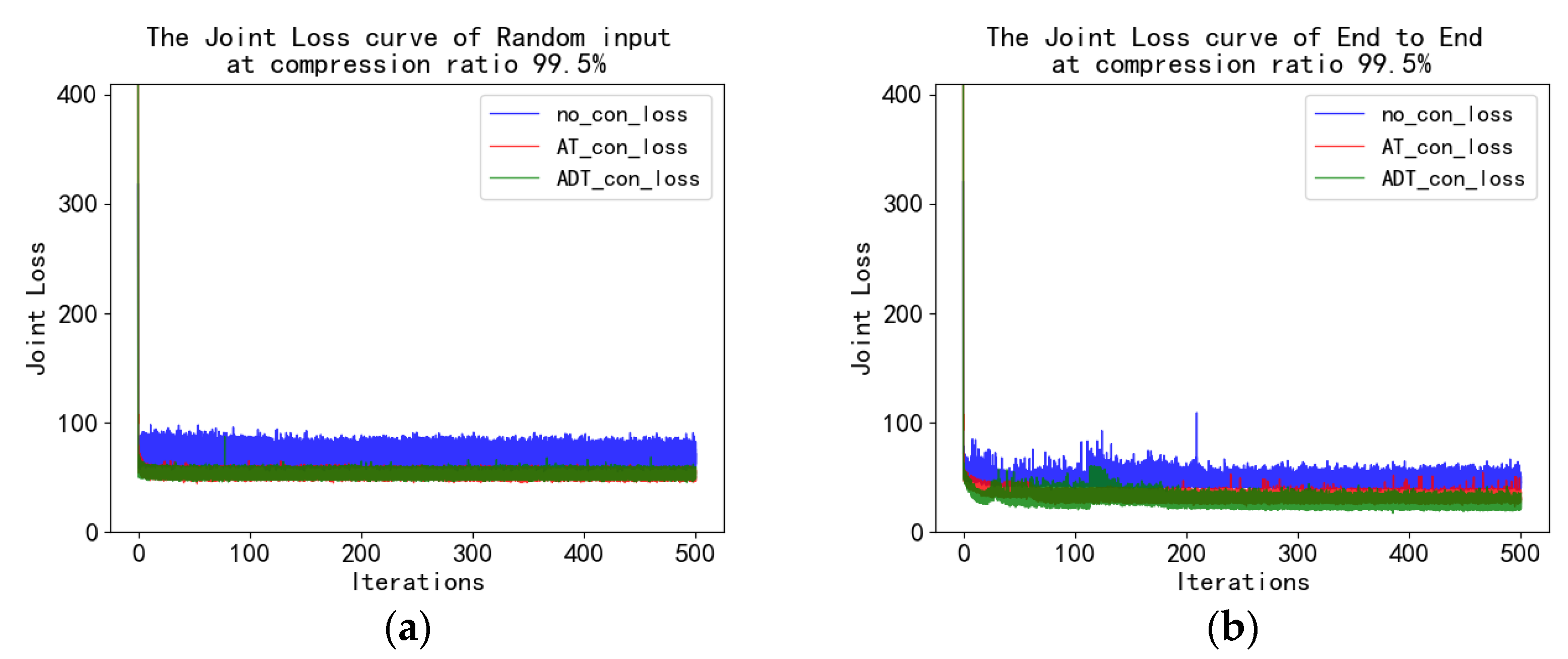
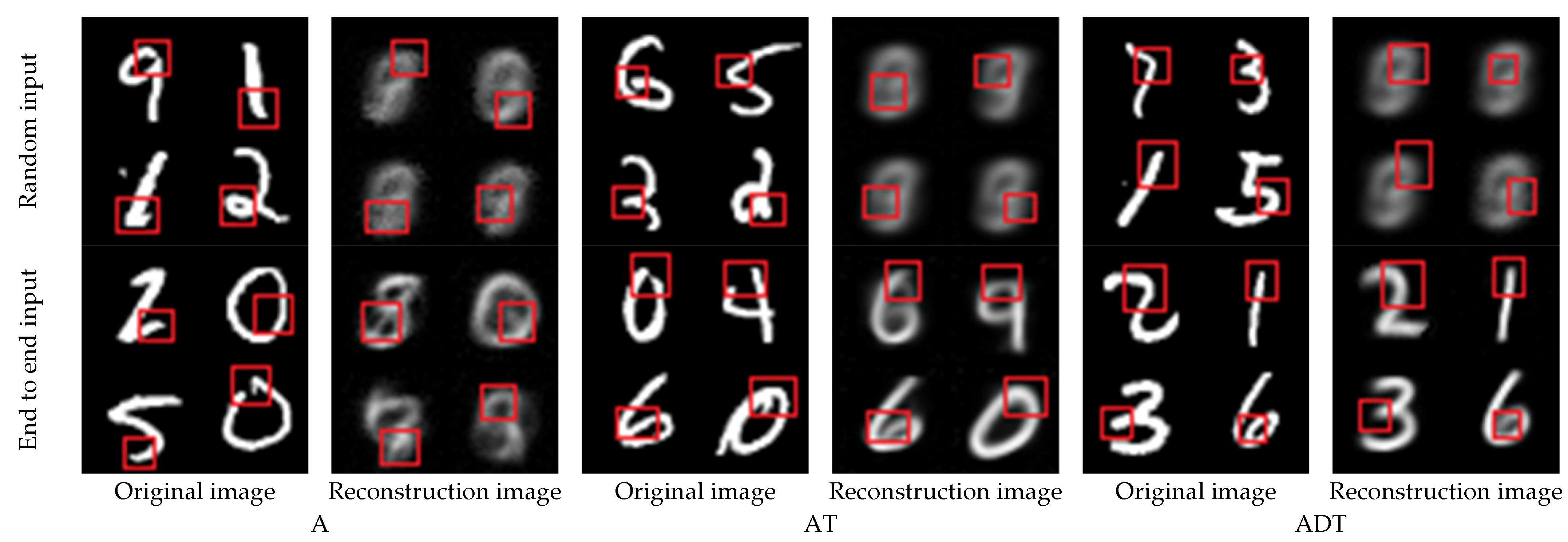
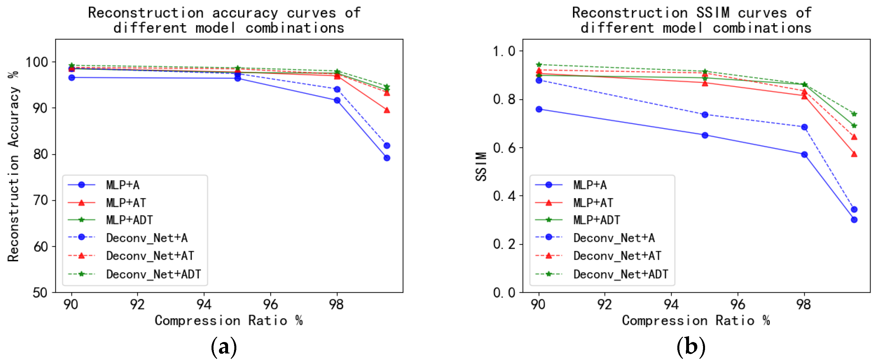
4.4. MNIST Experiment and Analysis

The experiments in this section mainly verify the feasibility of our proposed end-to-end correspondence relationship during the reconstruction process. Therefore, we used the same MLP generative model as DCS in all the reconstruction processes of the experiments in this section. In contrast to DCS’s random input, we used end-to-end to establish correspondence. This is fixing the input. In the reconstruction experiment of the MNIST dataset, the observed original data was 28 × 28. A, AT, and ADT were used as observation models. And the MLP was used as a generative model with the scale of sensing_dim-256-512-784. Reconstruction was performed at compression ratios of 75%, 80%, 85%, 90%, 95%, 98%, and 99.5% (the observation dimensions were 196, 157, 118, 78, 39, 16, and 4 (extreme observation)).
Figure 2 shows the reconstructed accuracy curve and SSIM curve under different compression ratios using the method we proposed for end-to-end correspondence establishment. MLP is the generation model, and A, AT, and ADT are three observation models. It can be seen that the compression ratio of 85% is the boundary. When the compression ratio is lower than 85%, the reconstruction effect after observation using A, AT, and ADT is similar. When the compression ratio is above 85%, the ADT reconstruction effect is better than that of AT and A.
Table 7 shows more detailed values. It can be seen that reconstruction accuracy is higher than 99% and SSIM is higher than 0.90 within the 85% compression rate. When the compression ratio was 90% (the observation dimension was 78), the reconstruction accuracy of ADT observation was 99.6%, which was similar to the reconstruction effect of AT, and 0.55% higher than that of A. Moreover, the SSIM of ADT was 0.9817, which was 0.0042 higher than AT and 0.06 higher than A. When the compression ratio was 95% (the observation dimension was 39), the reconstruction accuracy of ADT was 99.48%, which was 0.21% higher than AT and 1.52% higher than A. Furthermore, the SSIM of ADT was 0.9775, which was 0.0116 higher than AT and 0.3778 higher than A. When the compression ratio was 98% (the observation dimension was 16), the reconstruction accuracy of ADT was 98.45%, which was 0.54% higher than AT and 4.61% higher than A. The SSIM of ADT was 0.9353, which was 0.0345 higher than AT and 0.3452 higher than A. Figure 3 shows the reconstruction results of our proposed method. The details of the reconstructed image and the original image can be seen in the marked red boxes. The high reconstruction accuracy and reconstruction details demonstrate the feasibility of the proposed method.
To further research the efficacy of the proposed method, we continue to study the reconstruction of extreme observations. As shown in Table 7, the compression ratio was [(784 − 4)/784] × 100% ≈ 99.5%. When the observation dimension was 4 with the end-to-end method, the reconstruction accuracy of ADT was 91.61%, which was 2.07% better than AT and 4.54% better than A. The SSIM of ADT was 0.7032, which was 0.1185 higher than AT and 0.2515 higher than A. When random input of dimension 4 was used, the reconstruction accuracy of ADT was 83.86%, the reconstruction accuracy of AT was 84.95%, and the reconstruction accuracy of A was 83.80%. Their SSIM were all below 0.4. As shown in Figure 4, it can be seen intuitively that the end-to-end reconstruction accuracy and SSIM are better those that of random input. Figure 5 shows the training loss curves of the end-to-end method and random input; the end-to-end method’s loss curve is significantly lower than that of random input. As shown in the average loss in Table 8, the average difference in numerical values is 22.2930. As shown in Figure 6, the first line is the reconstruction effect of random input with dimension 4, and the reconstruction effect of extreme observation is blurry and unsharp. The second line is the end-to-end reconstruction effect. From the perspective of the reconstruction image, the reconstructed image after the observation of A is blurry, and the same image contains many contours of other images, which are almost unrecognizable. Although the image reconstructed after using AT is blurry, the digit can be distinguished compared with the A reconstruction, and some reconstruction effects are still blurry. Compared with the A and AT reconstructions, the reconstructed image using ADT has a high definition.
The convergence response of the end-to-end method was very rapid, and the clearer and identifiable images were reconstructed almost in about 15 epochs, and the loss of ADT reconstruction was lower than that of AT and A. Figure 3 and Figure 6 also proved the ADT reconstruction effect is better than that of AT and A. In Figure 6, the details and differences between the reconstructed and original images can be seen in the marked red boxes.
In the experiment in this section, end-to-end was used in the reconstruction experiment of MNIST. The compression ratio of 85% was the boundary. When the compression ratio was lower than 85%, the reconstruction effect was similar to that of A, AT, and ADT under the condition that MLP was used as the generative model. However, compared with AT and ADT, A had less computation and more flexible code operations. In the case of similar reconstruction results, the low computational cost shows apparent advantages. When the compression ratio was higher than 85%, the reconstruction effect of ADT was significantly better than that of AT and A and only needed about 15 epochs for rough reconstruction.
In contrast, the higher accuracy of reconstruction in a short time shows an advantage over the lower-dimensional observation reconstruction. With the compression ratio at 99.5% of the extreme observation, the reconstruction accuracy of the end-to-end method improved by 5.20% on average compared with the random input of DCS, and the SSIM improved by 0.22 on average. That verified the feasibility of the extreme observation and reconstruction method and showed that the end-to-end reconstruction method had excellent elasticity in the observation dimension.

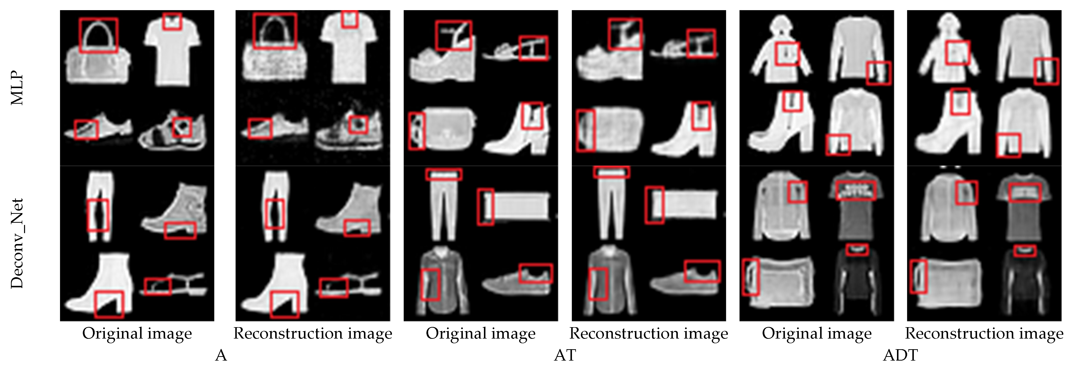
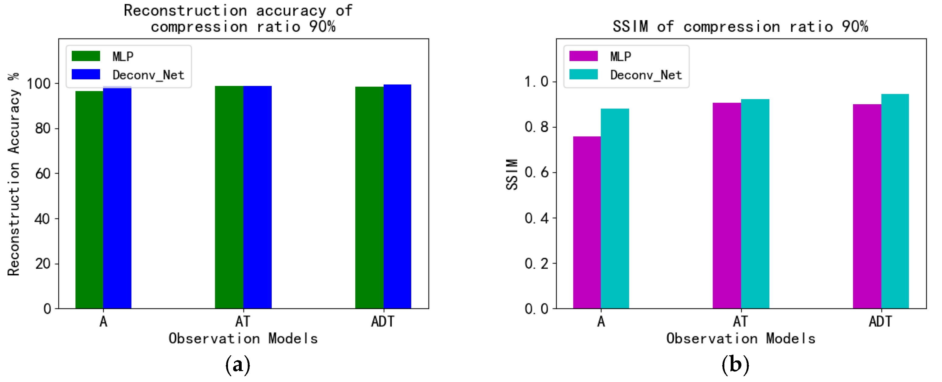
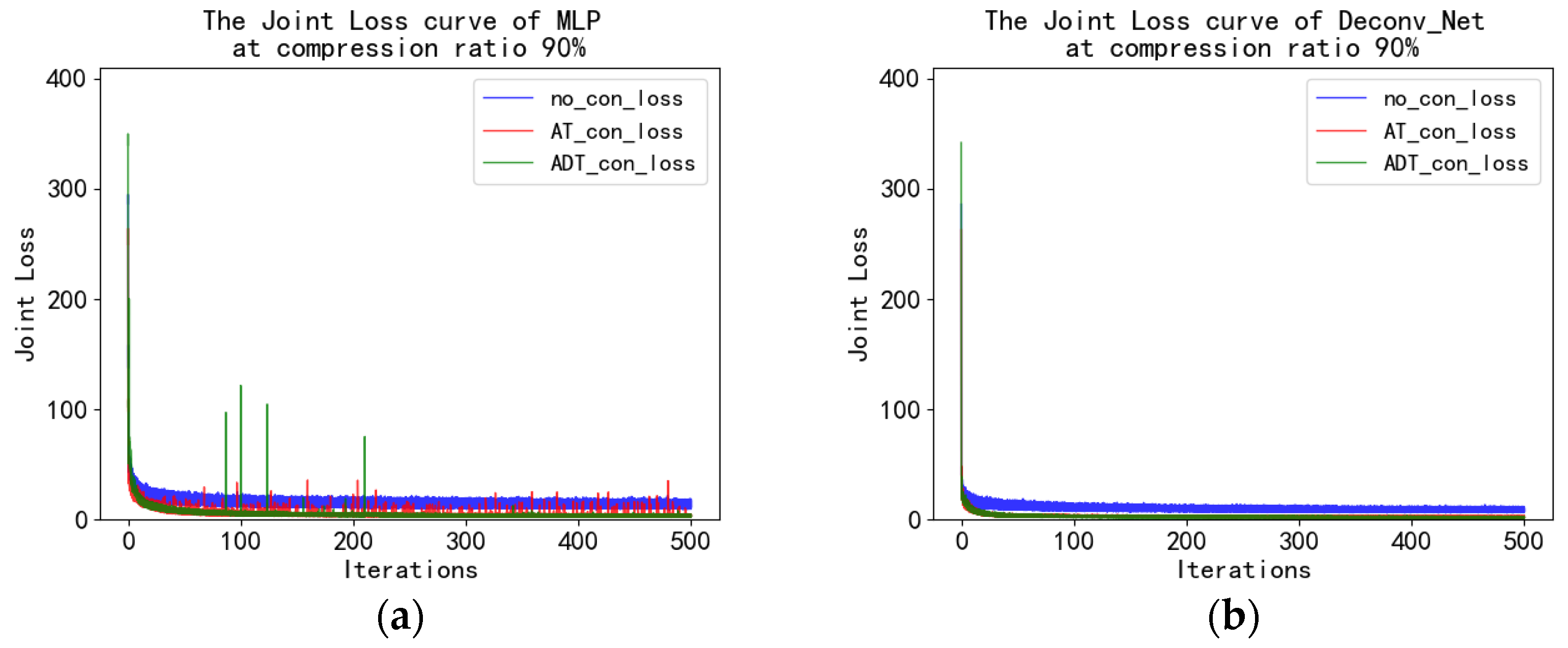
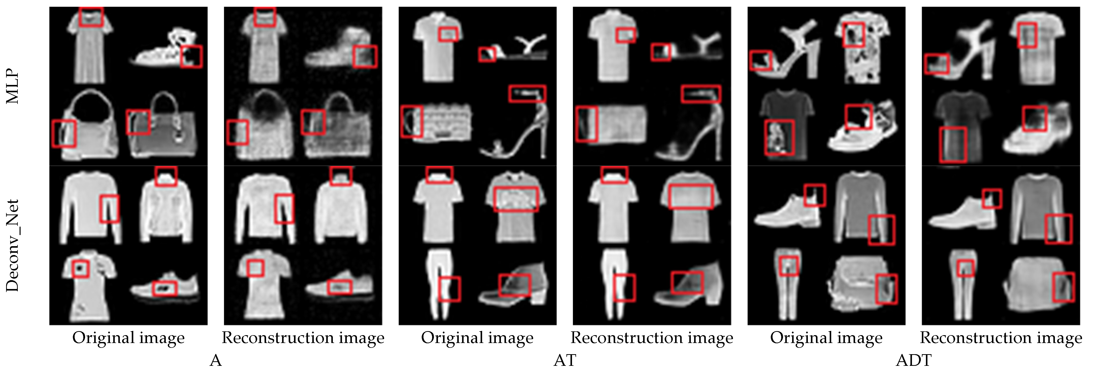
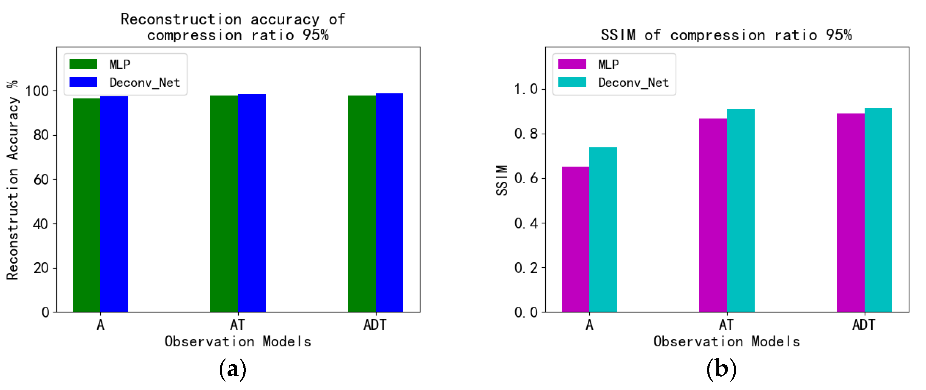
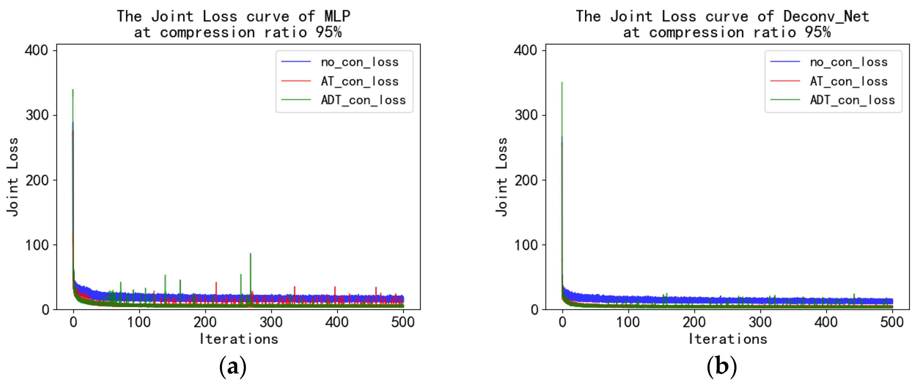
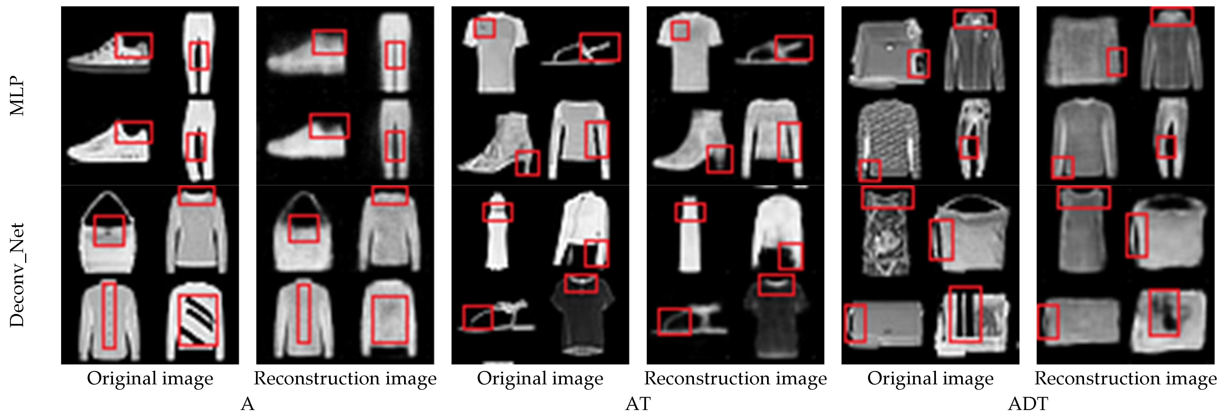
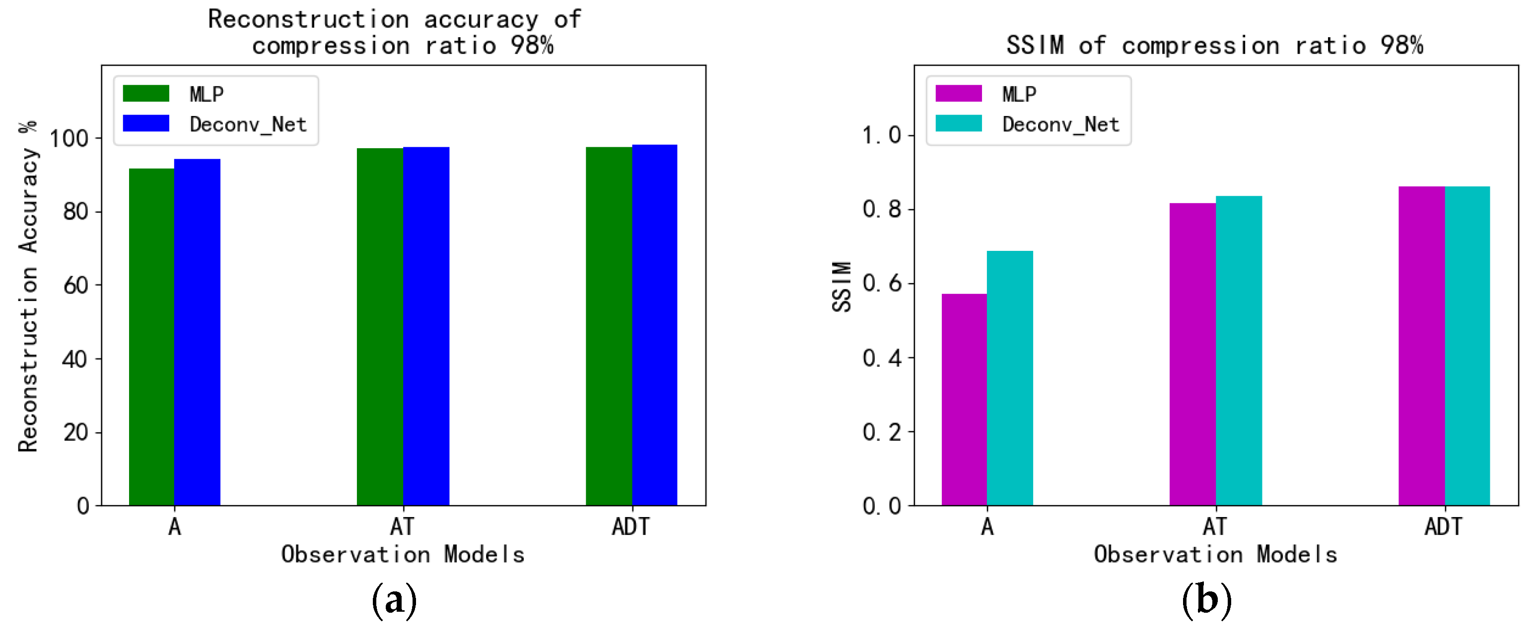
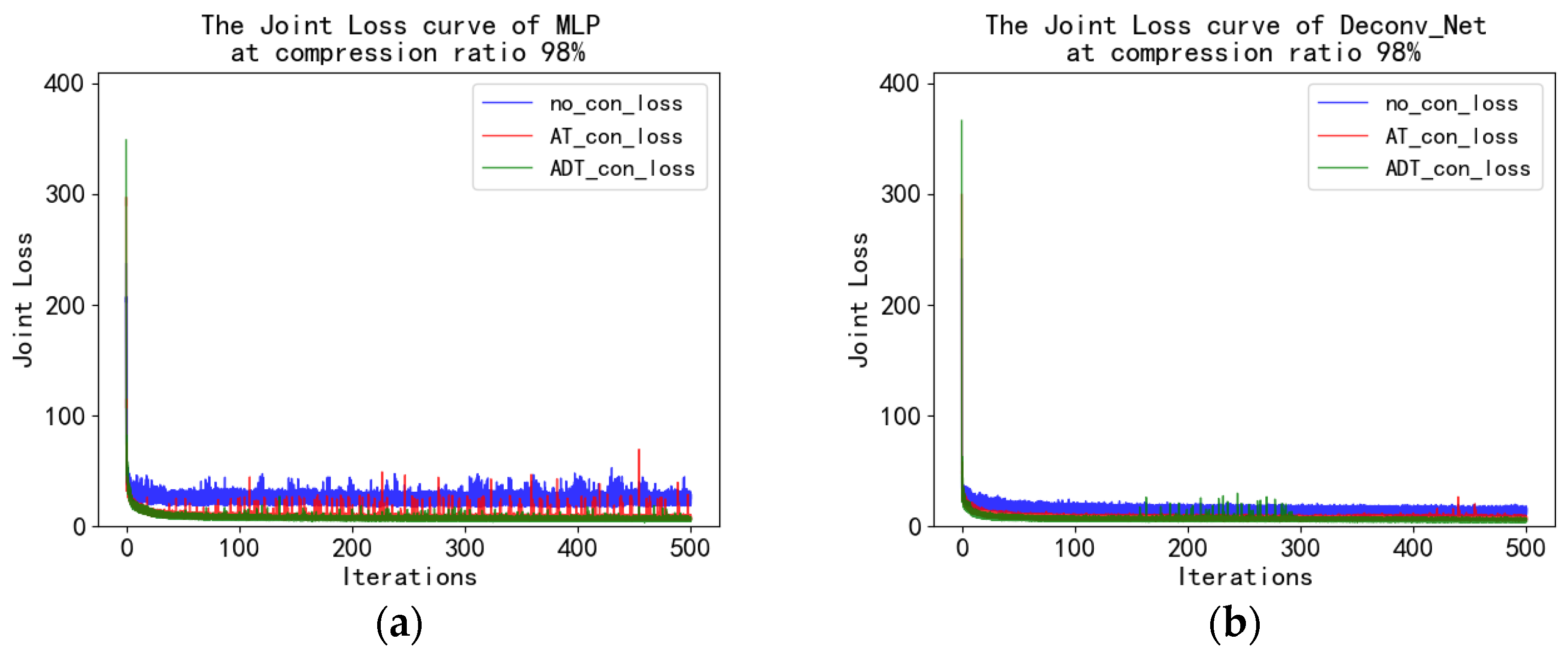
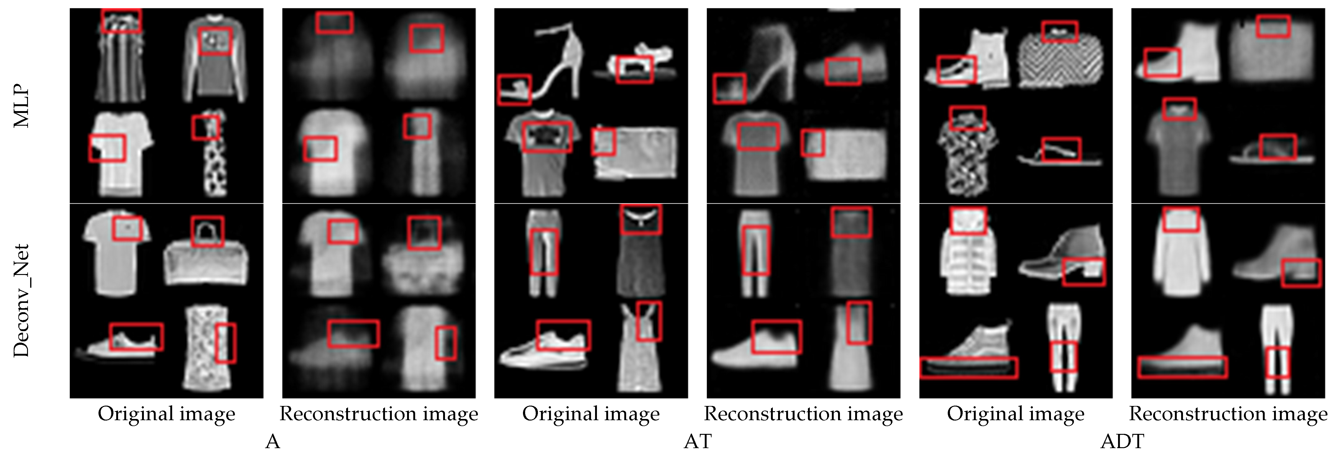
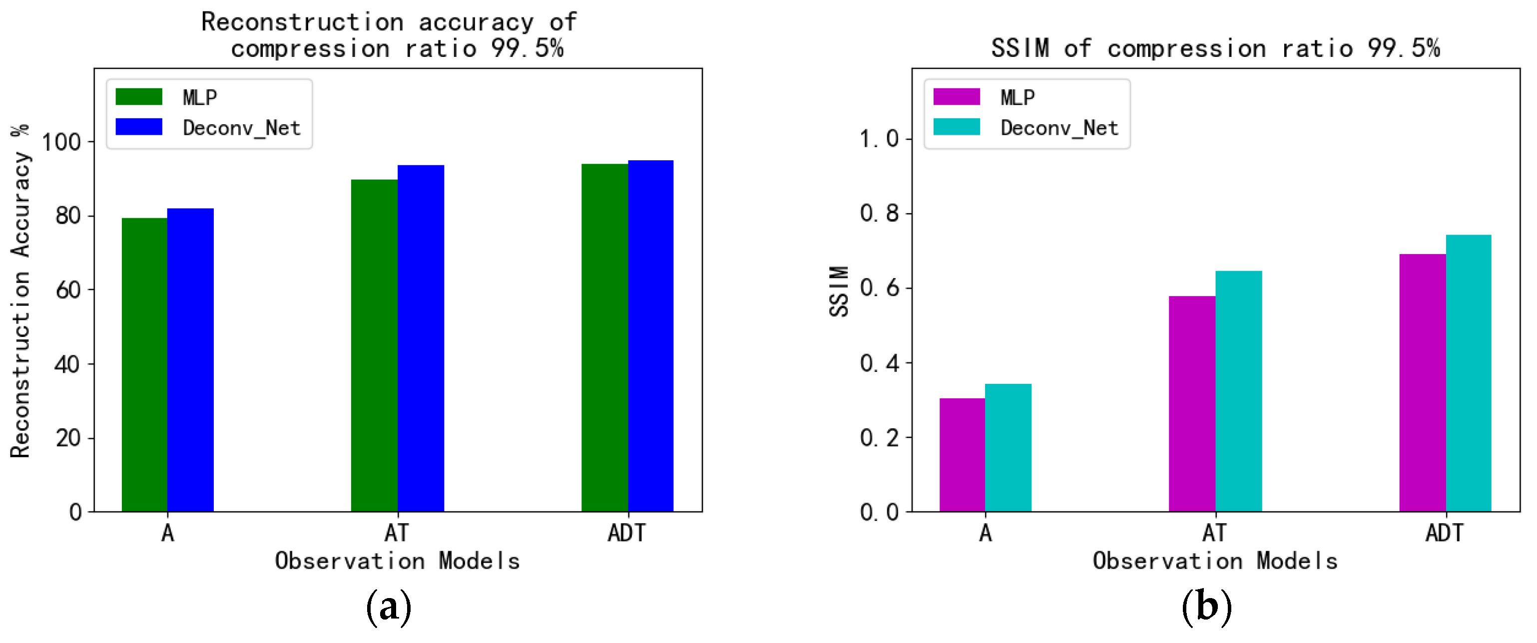
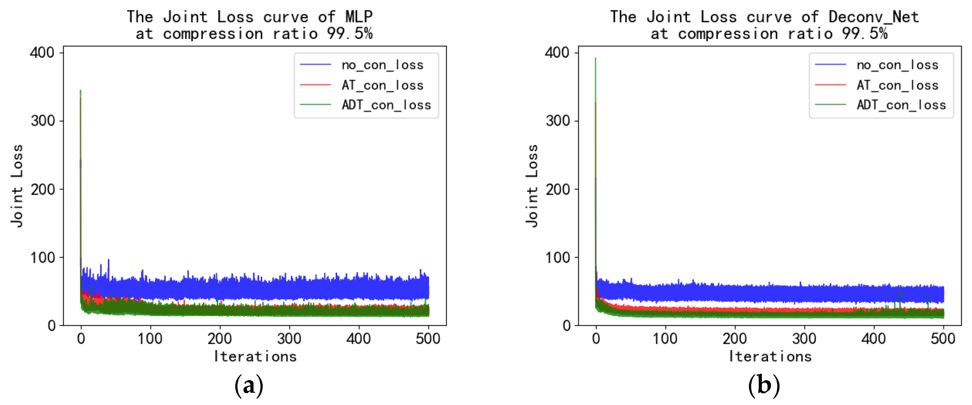
4.5. Fashion_MNIST Experiment and Analysis

In the experiments in the previous section, the feasibility of our proposed end-to-end correspondence relationship for reconstruction was verified. The end-to-end reconstruction is better than random input. However, to further improve the reconstruction effect, the structure of the generative model has become our focus.
Although the original data in the S-REC condition are free from the sparsity requirement, the handwritten digits of MNIST have noticeable foreground and background, making the MNIST dataset have inherent sparsity. Therefore, the Fashion_MNIST dataset was used in this section.
In the end-to-end reconstruction experiment of the Fashion_MNIST dataset, the observed original data was 28 × 28. The observation models used were A, AT, and ADT. The generative model of the experimental group was a Deconv_Net, and the control group was an MLP in DCS. According to the experimental results in Section 4.4., when the compression ratio was lower than 85%, the AT and ADT reconstruction advantage was not as good as that of A. Therefore, only the reconstruction of the low observation dimension was performed in this section, and the reconstruction was performed at the compression ratios of 90%, 95%, 98%, and 99.5% (the observation dimension was 78, 39, 16, and 4 (extreme observation)).
As shown in Figure 7, reconstruction accuracy curves and SSIM curves of different model combinations under different compression ratios are obtained. It can be seen from the trend that the reconstruction accuracy and SSIM of Deconv_Net+ADT are at high levels under different compression ratios. The reconstruction accuracy and SSIM of MLP+A are lower under different compression ratios.
Table 9 shows more detailed values. When the compression ratio was 90% (the observation dimension was 78), the reconstruction accuracy of the Deconv_Net was 3% higher than that of the MLP on average under different observation models, and the SSIM was 0.1797 higher than that. The best performance was the combination of the deconvolution generative model and the deep observation model (ADT), with a reconstruction accuracy of 99.23% and an SSIM of 0.9427. When the compression ratio was 95% (the observation dimension was 39), the reconstruction accuracy of the Deconv_Net was 2.74% higher than the MLP on average, and the SSIM was 0.1521 higher than that. The best performance was the combination of the deconvolution generative model and the deep observation model (ADT), with a reconstruction accuracy of 98.67% and an SSIM of 0.9152. When the compression ratio was 98% (the observation dimension was 16), the reconstruction accuracy of the Deconv_Net was 3.34% higher than the MLP on average, and the SSIM was 0.1346 higher than that. The best performance was the combination of the deconvolution generative model and the deep observation model (ADT), with a reconstruction accuracy of 98.00% and an SSIM of 0.8618. When the compression ratio was 99.5% (the observation dimension was 4), the reconstruction accuracy of the Deconv_Net was 2.49% higher than the MLP on average, and the SSIM was 0.1595 higher than that. The best performance was the combination of the deconvolution generative model and deep observation model (ADT), with a reconstruction accuracy of 94.74% and an SSIM of 0.7405. It can also be concluded from the accuracy and SSIM curve that the combination of the deconvolution generative model and deep observation model (ADT) is optimal. In summary, the combination of the deconvolution generative model and the deep observation model has a good reconstruction effect.
The reconstruction effects are shown in Figure 8, Figure 11, Figure 14 and Figure 17. The first row of all figures is the end-to-end reconstruction result of the MLP generative model, and the second row is the end-to-end reconstruction result of the Deconv_Net generative model. It can be seen intuitively that the accuracy and SSIM of the reconstructed image are relatively high in the two modes at lower compression ratios.
The reconstructed image with a 90% compression ratio is shown in Figure 8. Columns one, three, and five in Figure 8 are the original images, and columns two, four, and six are the restored images of different models. In Figure 8, the details of the reconstructed image and the original image can be noticed from the red marked boxes. The reconstructed image contains many details of the original image.
Figure 9 is a histogram of reconstruction accuracy and SSIM of different models when the compression rate is 90%. It can be seen that there is not much difference.
Figure 10 shows the loss curves for different models. Through the loss curve, it is found that there is no significant difference in the value of reconstruction loss after observation using A, AT, and ADT. However, Deconv_Net’s loss curve was more stable than MLP’s. This also shows that Deconv_Net generalization ability is better than MLP for reconstructing all datasets.
The reconstructed image with a compression ratio of 95% is shown in Figure 11. Columns one, three, and five in Figure 11 are the original images, and columns two, four, and six are the restored images of different models. In Figure 11, the details of the reconstructed image and the original image can be noticed from the red marked boxes. The reconstructed image contains many details of the original image.
Figure 12 is a histogram of reconstruction accuracy and SSIM for different models when the compression rate is 95%. It can be seen that there is not much difference in the reconstruction accuracy, but the SSIM of Deconv is higher than that of MLP.
Figure 13 shows the loss curves for different models. Similarly, through the loss curve, it is found that there is no significant difference in the value of reconstruction loss after observation using A, AT, and ADT. However, Deconv_Net’s loss curve was more stable than MLP’s. This also shows that Deconv_Net generalization ability is better than MLP for reconstructing all datasets.
The reconstructed image with a compression ratio of 98% is shown in Figure 14. Columns one, three, and five in Figure 14 are the original images, and columns two, four, and six are the restored images of different models. In Figure 14, the details and differences between the reconstructed and original images can be seen in the marked red boxes. The details of the reconstructed image become slightly blurred.
Figure 15 is a histogram of the reconstruction accuracy of different models when the compression rate is 98%. It can be seen that the reconstruction accuracy and SSIM of Deconv are slightly higher than those of MLP.
Figure 16 is the loss curve for different models. When MLP is the generation model, the reconstructed loss curve after observation with A, AT, and ADT fluctuates greatly and is very unstable. The loss curve of Deconv_Net was more stable than that of MLP. This suggests that Deconv_Net has been shown to generalize the fitted datasets better than MLP as the compression ratio increases.
The reconstructed image with a compression ratio of 99.5% is shown in Figure 17. Columns one, three, and five in Figure 17 are the original images, and columns two, four, and six are the restored images of different models. In Figure 17, the details and differences between the reconstructed and original images can be seen in the marked red boxes. The details of the reconstructed image of A become blurred, while AT and ADT still maintain contours and details.
Figure 18 is a histogram of the reconstruction accuracy for different models when the compression rate is 99.5%. It can be seen that the reconstruction accuracy and SSIM of Deconv are significantly higher than those of MLP.
Figure 19 is the loss curve for different models. When MLP is the generation model, the reconstructed loss curve after observation with A, AT, and ADT has a significant fluctuation and is very unstable. The loss curve of Deconv_Net was more stable than that of MLP. It can be seen from the loss curves of both models that the loss curves observed by ADT are significantly lower than those of A and AT. Again, Deconv_Net shows a better generalization of all fitted datasets than MLP as the compression ratio increases.
In the extreme observation a the dimension of four, the loss tends to be stable over a small number of epochs, and a relatively clear reconstruction image is obtained. Moreover, the loss curve of the Deconv_Net is significantly more stable than that of the MLP. It indicates the relative stability of the end-to-end correspondence.
This section also concludes that the higher the number of observation dimensions, the closer the reconstruction accuracy of A, AT, and ADT. The more no difference between the reconstruction effect and the reconstruction accuracy can be guaranteed above 96%. In this case, the reconstruction method combining A with the generative model with a lower cost can be selected. As the observation dimension becomes smaller and smaller, the observation vector seems to “condense” the original signal, and a minimal amount of observation signal carries a massive amount of information about the original signal. In the reconstruction experiments of different observation models, the reconstruction accuracy of the Deconv_Net generative model is 1.38% higher than that of the MLP generation model of DCS, and the SSIM is 0.0522 points higher than that. When the extreme observation with a compression ratio is 99.5% (the observation dimension is 4), the reconstruction accuracy of the Deconv_Net generative model is 2.49% higher than that of the MLP generative model of DCS, and the SSIM is 0.0532 higher than that. It also shows that the combination of the deconvolution generative model and the multi-layer perceptron observation model provides a higher possibility for the high-precision reconstruction of the observed image by establishing the corresponding relationship from end-to-end.

5. Conclusions

First of all, for the reconstruction of extreme observations, the end-to-end correspondence method proposed by us shows a very obvious reconstruction effect in MNIST dataset experiments compared with the random input of CSGM and DCS. The reason is that it is difficult to find random variables in the latent space that match the corresponding reconstructions during the reconstruction of extreme observations. Our idea is to directly use the low-dimensional vector of extreme observation to correspond with the observed original data for reconstruction. RIP and S-REC provide a guarantee for establishing the corresponding relationship. Secondly, in the end-to-end framework, the method of us combining the deconvolution generative model with the observation model is compared with the method of DCS combining the multi-layer perceptron generative model with the observation model. The reconstruction accuracy is improved by 1.38%, and the SSIM is improved by 0.0522 on average. The reconstruction accuracy of the extreme observation is improved by 2.49%, and the SSIM is improved by 0.0532 on average. The deep observation model of a multi-layer perceptron and the deconvolution generation model show excellent reconstruction performance. Since, in the deep observation model of a multi-layer perceptron, the dimension reduction of each hidden layer is constrained by RIP, different original signals will not be mapped to the same observation vector. At the same time, the generative model is also subject to RIP constraints: different observation vectors will not map to the same reconstruction signal, which provides a guarantee for the reconstruction of extreme observations. In the hidden layer structure of the generative model, the deconvolution generation model is different from the multilayer perceptron. The feature map of the deconvolution network carries the spatial information of the image, so in the extreme, the feature map of the hidden layer of the convolution network carries more data features than the linear connection of the multilayer perceptron, which is beneficial to the reconstruction of image data.
Generalization ability is commonly mentioned in machine learning, and overfitting is a key obstacle in machine learning that is not easy to overcome. In this paper, the generative neural network model was used to reconstruct compressed sensing, which was a lossy reconstruction process. The reconstruction process precisely uses the disadvantage of overfitting to improve the reconstruction’s accuracy. In future research, we will continue exploring methods for the high-precision reconstruction of low-dimensional observations and combine this method with application scenarios.

Author Contributions

Conceptualization, X.L.; methodology, H.D.; software, H.D.; validation, H.D. and C.F.; formal analysis, H.D.; investigation, H.D.; resources, X.L.; data curation, X.L.; writing—original draft preparation, H.D.; writing—review and editing, C.F.; visualization, C.F.; supervision, X.L. and C.F.; project administration, X.L.; funding acquisition, X.L. All authors have read and agreed to the published version of the manuscript.

Funding

This work was supported by the Cross-Disciplinary Science Foundation from Beijing Institute of Petrochemical Technology (Project No. BIPTCSF-21).

Institutional Review Board Statement

Not applicable.

Informed Consent Statement

Not applicable.

Data Availability Statement

The data used in this study including the MNIST and Fashion_MNIST image sets are openly available.

Conflicts of Interest

The authors declare no conflict of interest.

References

  1. Shi, G.M.; Liu, D.H.; Gao, D.H.; Liu, Z.; Lin, J.; Wang, L.J. Advances in Theory and Application of Compressed Sensing. Acta Electron. Sin. 2009, 37, 1070–1081. [Google Scholar]
  2. Donoho, D.L. Compressed sensing. IEEE Trans. Inf. Theory 2006, 52, 1289–1306. [Google Scholar] [CrossRef]
  3. Zeng, C.Y.; Ye, J.X.; Wang, Z.F.; Wu, M. Survey of compressed sensing reconstruction algorithms in deep learning framework. Comput. Eng. Appl. 2019, 55, 1–8. [Google Scholar]
  4. Jiao, L.C.; Yang, S.Y.; Liu, F.; Hou, B. Development and Prospect of Compressive Sensing. Acta Electron. Sin. 2011, 39, 1651–1662. [Google Scholar]
  5. Tauböck, G.; Hlawatsch, F. A compressed sensing technique for OFDM channel estimation in mobile environments: Exploiting channel sparsity for reducing pilots. In Proceedings of the 2008 IEEE International Conference on Acoustics, Speech and Signal Processing, Las Vegas, NV, USA, 31 March–4 April 2008; pp. 2885–2888. [Google Scholar]
  6. Bajwa, W.U.; Haupt, J.D.; Sayeed, A.M.; Nowak, R.D. Joint Source–Channel Communication for Distributed Estimation in Sensor Networks. IEEE Trans. Inf. Theory 2007, 53, 3629–3653. [Google Scholar] [CrossRef]
  7. Lustig, M.; Donoho, D.L.; Pauly, J.M. Sparse MRI: The application of compressed sensing for rapid MR imaging. Magn. Reson. Med. 2007, 58, 1182–1195. [Google Scholar] [CrossRef]
  8. Provost, J.; Lesage, F. The Application of Compressed Sensing for Photo-Acoustic Tomography. IEEE Trans. Med. Imaging 2009, 28, 585–594. [Google Scholar] [CrossRef]
  9. Jung, H.; Sung, K.; Nayak, K.S.; Kim, E.Y.; Ye, J.C. k-t FOCUSS: A general compressed sensing framework for high resolution dynamic MRI. Magn. Reson. Med. 2009, 61, 103–116. [Google Scholar] [CrossRef]
  10. Kim, Y.; Narayanan, S.S.; Nayak, K.S. Accelerated three-dimensional upper airway MRI using compressed sensing. Magn. Reson. Med. 2009, 61, 1434–1440. [Google Scholar] [CrossRef] [Green Version]
  11. Hu, S.; Lustig, M.; Chen, A.P.; Crane, J.C.; Kerr, A.B.; Kelley, D.A.; Hurd, R.E.; Kurhanewicz, J.; Nelson, S.J.; Pauly, J.M.; et al. Compressed sensing for resolution enhancement of hyperpolarized 13C flyback 3D-MRSI. J. Magn. Reson. 2008, 192, 258–264. [Google Scholar] [CrossRef] [Green Version]
  12. Herman, M.A.; Strohmer, T. High-Resolution Radar via Compressed Sensing. IEEE Trans. Signal Process. 2009, 57, 2275–2284. [Google Scholar] [CrossRef] [Green Version]
  13. Bobin, J.; Starck, J.; Ottensamer, R. Compressed Sensing in Astronomy. IEEE J. Sel. Top. Signal Process. 2008, 2, 718–726. [Google Scholar] [CrossRef] [Green Version]
  14. Shamsi, D.; Boufounos, P.T.; Koushanfar, F. Noninvasive leakage power tomography of integrated circuits by compressive sensing. In Proceedings of the 13th International Symposium on Low Power Electronics and Design (ISLPED ‘08), Bangalore, India, 11–13 August 2008; pp. 341–346. [Google Scholar]
  15. Wright, J.; Yang, A.Y.; Ganesh, A.; Sastry, S.S.; Ma, Y. Robust Face Recognition via Sparse Representation. IEEE Trans. Pattern Anal. Mach. Intell. 2009, 31, 210–227. [Google Scholar] [CrossRef]
  16. Elad, M. Optimized Projections for Compressed Sensing. IEEE Trans. Signal Process. 2007, 55, 5695–5702. [Google Scholar] [CrossRef]
  17. Calderbank, R. Compressed Learning: Universal Sparse Dimensionality Reduction and Learning in the Measurement Domain; Technical Report; Rice University: Houston, TX, USA, 2009. [Google Scholar]
  18. Duarte, M.F.; Davenport, M.A.; Takhar, D.; Laska, J.N.; Sun, T.; Kelly, K.F.; Baraniuk, R. Single-Pixel Imaging via Compressive Sampling. IEEE Signal Process. Mag. 2008, 25, 83–91. [Google Scholar] [CrossRef] [Green Version]
  19. Bora, A.; Jalal, A.; Price, E.; Dimakis, A.G. Compressed Sensing using Generative Models. In Proceedings of the International Conference on Machine Learning, Sydney, Australia, 6–11 August 2017. [Google Scholar]
  20. Kingma, D.P.; Welling, M. Auto-Encoding Variational Bayes. arXiv 2014, arXiv:1312.6114. [Google Scholar]
  21. Goodfellow, I.J.; Pouget-Abadie, J.; Mirza, M.; Xu, B.; Warde-Farley, D.; Ozair, S.; Courville, A.C.; Bengio, Y. Generative Adversarial Nets. In Neural Information Processing Systems; MIT Press: Cambridge, MA, USA, 2014. [Google Scholar]
  22. Mardani, M.; Gong, E.; Cheng, J.Y.; Vasanawala, S.S.; Zaharchuk, G.; Alley, M.T.; Thakur, N.; Han, S.; Dally, W.J.; Pauly, J.M.; et al. Deep Generative Adversarial Networks for Compressed Sensing Automates MRI. arXiv 2017, arXiv:1706.00051. [Google Scholar]
  23. Veen, D.V.; Jalal, A.; Price, E.; Vishwanath, S.; Dimakis, A.G. Compressed Sensing with Deep Image Prior and Learned Regularization. arXiv 2018, arXiv:1806.06438. [Google Scholar]
  24. Wu, Y.; Rosca, M.; Lillicrap, T.P. Deep Compressed Sensing. In Proceedings of the International Conference on Machine Learning, Long Beach, CA, USA, 10–15 June 2019. [Google Scholar]
  25. Sun, Y.; Chen, J.; Liu, Q.; Liu, G. Learning image compressed sensing with sub-pixel convolutional generative adversarial network. Pattern Recognit. 2020, 98, 107051. [Google Scholar] [CrossRef]
  26. Sheykhivand, S.; Rezaii, T.Y.; Meshgini, S.; Makoui, S.; Farzamnia, A. Developing a Deep Neural Network for Driver Fatigue Detection Using EEG Signals Based on Compressed Sensing. Sustainability 2022, 14, 2941. [Google Scholar] [CrossRef]
  27. Islam, S.R.; Maity, S.P.; Ray, A.K.; Mandal, M. Deep learning on compressed sensing measurements in pneumonia detection. Int. J. Imaging Syst. Technol. 2022, 32, 41–54. [Google Scholar] [CrossRef]
  28. Finn, C.; Abbeel, P.; Levine, S. Model-Agnostic Meta-Learning for Fast Adaptation of Deep Networks. arXiv 2017, arXiv:1703.03400. [Google Scholar]
Figure 1. Block diagram to the E2E_DCSGM structure.
Applsci 12 12176 g001
Figure 2. (a) Reconstruction accuracy curves of different model combinations; (b) Reconstruction SSIM curves of different model combinations.
Applsci 12 12176 g002
Figure 3. Experimental results of MNIST reconstruction.
Applsci 12 12176 g003
Figure 4. (Comparison of reconstruction accuracy (a) and SSIM (b) between random input and end-to-end.
Applsci 12 12176 g004
Figure 5. The joint loss curves for (a) random input and (b) end-to-end.
Applsci 12 12176 g005
Figure 6. Comparison of reconstructed images of extreme observations.
Applsci 12 12176 g006
Figure 7. Reconstruction accuracy (a) and SSIM (b) curves of different model combinations.
Applsci 12 12176 g007
Figure 8. Reconstruction results of a 90% compression ratio.
Applsci 12 12176 g008
Figure 9. Comparison of reconstruction accuracy (a) and SSIM (b) between MLP and Deconv at a 90% compression ratio.
Applsci 12 12176 g009
Figure 10. The joint loss curve with the end-to-end MLP model (a) and with the end-to-end Deconv_Net model (b) at a 90% compression ratio.
Applsci 12 12176 g010
Figure 11. Reconstruction results of at a 95% compression ratio.
Applsci 12 12176 g011
Figure 12. Comparison of (a) reconstruction accuracy and SSIM (b) between MLP and Deconv at a compression ratio of 95%.
Applsci 12 12176 g012
Figure 13. The joint loss curve with the end-to-end MLP model (a) and the end-to-end Deconv_Net model (b) at a 95% compression ratio.
Applsci 12 12176 g013
Figure 14. Reconstruction results of at a 98% compression ratio.
Applsci 12 12176 g014
Figure 15. Comparison of reconstruction accuracy (a) and SSIM (b) between MLP and Deconv at a compression ratio of 98%.
Applsci 12 12176 g015
Figure 16. The joint loss curve with the end-to-end MLP model (a) and the end-to-end Deconv_Net model (b) at a compression ratio of 98%.
Applsci 12 12176 g016
Figure 17. Reconstruction results of at a 99.5% compression ratio.
Applsci 12 12176 g017
Figure 18. Comparison of reconstruction accuracy (a) between MLP and Deconv and SSIM (b) at a compression ratio of 99.5%.
Applsci 12 12176 g018
Figure 19. The joint loss curve with the end-to-end MLP model (a) and the end-to-end Deconv_Net model (b) at a compression ratio of 99.5%.
Applsci 12 12176 g019
Table 1. Notations and their meanings.
NotationMeanings
x the original signal
Φ the observation model
y the observed vector
x ^ the generated signal
G θ the generative model
z the input of generative model from normalized the observed vector
z ^ the input that is optimized
y ^ the observed vector that is optimized
L 2 the Euclidean norm
L G the loss of generative model
L Φ the loss of observation model
α the inner loop optimization rate
β the outer loop optimization rate
θ the parameter of model
Tthe inner loop iteration
Nthe outer loop iteration
L o s s i n n e r _ l o o p the loss of inner loop
L o s s o u t e r _ l o o p the loss of outer loop
Table 2. Model combination of experimental and control groups.
MethodInputModels CombinationTypePurpose
CSGMRandom inputMLP + AControl GroupRandom input control group
DCSRandom inputMLP + ATControl Group
DCSMLP + ADT
We proposedend-to-endMLP + AExperimental GroupVerify the feasibility of end-to-end reconstruction under the extreme observation
MLP + AT
MLP + ADT
end-to-endDeconv_Net + AExperimental GroupVerify the reconstruction effect of the improved generator on the extreme observation under the end-to-end case
Deconv_Net + AT
Deconv_Net + ADT
Table 3. Hyperparameter Settings of multi-layer perceptron generative model.
Network LayerRelated Hyperparameter Settings
Inputbatch_size = 64
(batch_size, sensing_dim)
Hidden layer 1Linear(sensing_dim, 256)
activation function: LeakyReLU
Hidden layer 2Linear(256, 512)
activation function: LeakyReLU
Hidden layer 3Linear(512, 784)
activation function: Tanh
output(batch_size,1, 28, 28)
Table 4. Hyperparameter Settings of deconvolution generative model.
Network LayerRelated Hyperparameter Settings
Inputbatch_size = 64
(batch_size, sensing_dim)
upsampling 1scale_factor: 2
deconvolution layer 1kernel_size: (128, 3 × 3), stride_size: 1, padding_size: 1
activation function: LeakyReLU
upsampling 2scale_factor: 2
deconvolution layer 2kernel_size: (64, 3 × 3), stride_size: 1, padding_size: 1
activation function: LeakyReLU
deconvolution layer 3kernel_size: (1, 3 × 3), stride_size: 1, padding_size: 1
activation function: Tanh
output(batch_size, 1, 28, 28)
Table 5. Hyperparameter Settings of multi-layer perceptron deep observation network.
Network LayerRelated Hyperparameter Settings
Inputbatch_size = 64
(batch_size,1, 28, 28)
Hidden layer 1Linear(784, 512)
activation function: LeakyReLU
Hidden layer 2Linear(512, 256)
activation function: LeakyReLU
Hidden layer 3Linear(256, sensing_dim)
output(batch_size, sensing_dim)
Table 6. Experiment operating environment.
CategoryVersions
operating systemWindows10
CPUCore i5-10400 2.9 GHz
GPUNVIDIA RTX2070SUPER 8G
Pythonpython3.8
Pytorchpytorch1.10
CUDACUDA version10.2
cuDNNcuDNN7.6.5
Table 7. Comparison of MNIST reconstruction accuracy and SSIM.
Compression Ratio
(Number of Observations)
75% (196)80% (157)85% (118)90% (78)95% (39)98% (16)
AccuracySSIMAccuracySSIMAccuracySSIMAccuracySSIMAccuracySSIMAccuracySSIM
A99.76%0.974699.61%0.971099.54%0.970199.05%0.921797.96%0.599793.82%0.5901
AT99.76%0.982999.67%0.973199.68%0.978499.60%0.977599.27%0.965997.91%0.9008
ADT99.62%0.979499.72%0.986899.75%0.985999.60%0.981799.48%0.977598.45%0.9353
Table 8. Comparison of reconstruction results for extreme observations.
Observation ModelAATADT
Reconstruction accuracyrandom input83.80%84.95%83.86%
end-to-end input87.07%89.54%91.61%
SSIMrandom input0.34910.35010.3803
end-to-end input0.45170.58470.7032
Average lossrandom input70.339953.040253.2837
end-to-end input47.470233.837028.4777
Table 9. Comparison of Fashion_MNIST reconstruction accuracy results.
MethodCompression Ratio
(Number of Observations)
90% (78)95% (39)98% (16)99.5% (4)
AccuracySSIMAccuracySSIMAccuracySSIMAccuracySSIM
CSGMMLP + A96.57%0.758896.40%0.651891.63%0.572179.15%0.3026
DCSMLP + AT98.54%0.906197.75%0.868096.94%0.813989.58%0.5757
DCSMLP + ADT98.49%0.898097.65%0.887997.51%0.860293.88%0.6898
We proposedConv + A98.60%0.879397.42%0.736594.10%0.685081.94%0.3430
Conv + AT98.77%0.920698.45%0.908197.32%0.834093.40%0.6441
Conv + ADT99.23%0.942798.67%0.915298.00%0.861894.74%0.7405
Publisher’s Note: MDPI stays neutral with regard to jurisdictional claims in published maps and institutional affiliations.

