Anomaly Detection Method in Railway Using Signal Processing and Deep Learning

Abstract

In this paper, anomaly detection of wheel flats based on signal processing and deep learning techniques is analyzed. Wheel flats mostly affect running stability and ride comfort. Currently, domestic railway companies visually inspect wheel flats one by one with their eyes after railway vehicles enter the railway depots for maintenance. Therefore, CBM (Condition-Based Maintenance) is required for wheel flats resolution. Anomaly detection for wheel flat signals of railway vehicles using Order analysis and STFT (Short Time Fourier Transform) is studied in this paper. In the case of railway vehicles, it is not easy to obtain actual failure data through running vehicles in a university laboratory due to safety and cost issues. Therefore, vibration-induced acceleration was obtained using a multibody dynamics simulation software, SIMPACK. This method is also proved in the other paper by rig tests. In addition, since the noise signal was not included in the simulated vibration, the noise signal obtained from the Seoul Metro Subway Line 7 vehicle was overlapped with the simulated one. Finally, to improve the performance of both detection rate and real-time of characteristics based on existing LeNet-5 architectures, spectrogram images transformed from time domain data were proceeded with the LeNet deep learning model modified with the pooling method and activation function. As a result, it is validated that the method using the spectrogram with a deep learning approach yields higher accuracy than the time domain data.

1. Introduction

In the wheels of the railway vehicles, as shown in Figure 1, it is known that wheel flats are caused both by fatigue of rolling contact and frictional wear between the wheel and rail [1]. If wheel flat occurs, the bogie device may be damaged and the, running stability and ride comfort of the vehicle may also deteriorate. Therefore, corrective maintenance should be introduced in the event of a wheel flat.

Currently, in most cases, at the Seoul Metro in Korea, the wheel flats are visually inspected one by one by the railway maintenance staff. However, based on the example of a standard train composed of 10 units, the difficulty of checking 80 wheels is aggravated. In addition, according to the safety standards for urban railway vehicles, wheel turning is required in the case shown in

Table 1. Safety standards for domestic urban railway vehicles.

The Number of Wheel Flats [EA]	Flat Size [mm]
1	75 < Flat size
2	50 $\le$ Flat size < 75
4	25 $\le$ Flat size < 50

, reprinted from ref. [2].

However, when a person visually checks the wheels one by one, cases happen in which flats are missed, and wheel turning occurs frequently, even if it does not comply with the regulations. Due to this problem, work efficiency is degraded, and the life of the wheelset is also reduced. Therefore, it is necessary to develop CBM (Condition Based Maintenance) in order to increase work efficiency and wheel life sustainability. In addition, maintenance costs of over hundreds of millions of dollars ($) are being spent every year in the field of railway vehicles. Accordingly, if CBM is systematically applied, life cycle costs are expected to be reduced [3]. Hyundai Rotem, a local company in Korea, started developing CBM-related technology in 2018 and plans to complete the verification of availability and maintainability through domestic and overseas projects until 2024. It is expected that CBM adaptation will reduce the maintenance cost by up to 30% and increase the lifespan of the device by 40% [4].

K.Y.Kim used Cepstrum analysis to detect and diagnose wheel flats [5]. B.H. Park et al. studied tool condition diagnosis using the AlexNet model [6]. R.B. Randall analyzed vibration signals for rotating and reciprocating machines and defective defects using abnormal signals found in the analysis results [7]. Run Gao et al. proposed a method to detect the depth of a wheel flat according to vertical change due to a wheel flat by using the Parallelogram Mechanism to diagnose the wheel flat defects of railway vehicles [8]. B.Liang and S.Iwnicki et al. applied the Time-Frequency method to wheel flat detection [9]. Chunsheng Yang et al. detected defects in rails through supervised learning methods. Unlike in this paper, the features were extracted using the wavelet method. Moreover, the deep learning models used in this work are ResNet and FCN [10]. Praneeth Chandra et al. performed defect detection of rail clamps using Unsupervised Machine Learning. At this time, missing detection utilized the DBSCAN (Density-based spatial clustering of applications with noise) algorithm [11]. Praneeth Chandra et al. diagnosed defects using supervised machine learning. At this time, the learning data was obtained using the Eddy current sensor, and six machine learning models were used. As a result, it was confirmed that the result value was the best when the AdaBoost model was used [12]. K.Jahan et al. used semantic segmentation and supervised learning for anomaly detection in rail. At this time, the data was obtained through the camera [13]. Toshihide Yokouchi et al. performed a defect detection method for railway vehicle air conditioning. In this case, data from the Train Control and Monitoring System (TCMS) was used to detect defects, and they evaluated the normalities of vehicle equipment using a neural network with Long Short Term Memory (LSTM) [14]. N.Bosso et al. proposed a method to detect wheel flat defects by measuring the vertical acceleration on the axle box, and this method was verified by both simulation and test. At this time, the algorithm that the wheel flat index proposed was able to detect small flats and estimate their severity [15]. J.Brizuela et al. proposed a method to detect wheel flats using measurement by ultrasound. At this time, this paper differs from other approaches, using ultrasonic pulses (Rayleigh waves) being sent over a measuring rail; this method provides the loss of material and the length of the flat originally formed by abrasion [16].

In this paper, firstly, two signal processing methods and CNN (Convolutional Neural Networks) among the deep learning algorithms were used to study the anomaly detection method for wheel flat parts in CBM. At this time, anomaly detection was applied by classifying the normality and anomaly according to the safety standards of urban railway vehicles. Finally, through the anomaly detection method, the data with signal processing and the data without signal processing were compared using deep learning results. The deep learning results were confirmed through accuracy and ROC curve, together with the AUC value being confirmed through ROC curve.

2. Modeling of Railway Vehicles and Wheel Flat

2.1. Modeling of Railway Vehicles

The railway, which belongs to a public industry sector, is strongly linked to passenger safety and service, and it is not easy to conduct failure tests on actual operating railways. In other words, since an accident may occur while driving a broken-down vehicle on the railway, it was not allowed to conduct such a test using a broken-down train to detect anomalies for this study. Therefore, due to the difficulty of acquiring data through actual tests, simulation studies are applied in many research works and development projects in the field of railway vehicles.

In this study, SIMPACK, a multi-body dynamics software, was used to obtain wheel flat signals under various conditions. SIMPACK software with rail module has an advantage similar to the actual railway vehicle driving which considers the contact between the wheel and rail. The railway vehicle model in this study was generated with the Seoul Metro’s subway train in Korea.

Figure 2 shows a railway vehicle modeled by SIMPACK, a multi-body dynamics software, and Figure 3 shows the bogie modeling of a railway vehicle. The specifications of car body, bogie, and track information are shown in

Table 2. Modeling values of length and mass.

Parameters	Unit	Value
Car Body Length	(mm)	19,500
Car Body Width	(mm)	3120
Car Body Height	(mm)	3750
Car Body Mass	(ton)	1.73
Wheelbase	(mm)	2100
Bogie Mass	(ton)	2.185
Wheelset Mass	(ton)	1.647
Axle Box Mass	(ton)	0.16

,

Table 3. Modeling values of inertia and stiffness.

Parameters	Unit	Value
Car Body Ixx	($\mathrm{kg}·{\mathrm{m}}^2$)	25,757
Car Body Iyy	($\mathrm{kg}·{\mathrm{m}}^2$)	320,790
Car Body Izz	($\mathrm{kg}·{\mathrm{m}}^2$)	317,990
Bogie Ixx	($\mathrm{kg}·{\mathrm{m}}^2$)	848.1
Bogie Iyy	($\mathrm{kg}·{\mathrm{m}}^2$)	1376.3
Bogie Izz	($\mathrm{kg}·{\mathrm{m}}^2$)	2112.2
Wheelset Ixx	($\mathrm{kg}·{\mathrm{m}}^2$)	844
Wheelset Iyy	($\mathrm{kg}·{\mathrm{m}}^2$)	107
Wheelset Izz	($\mathrm{kg}·{\mathrm{m}}^2$)	844
Primary Suspension Stiffness	(N/m)	836,338
Secondary Suspension Stiffness	(N/m)	2,657,143

and

Table 4. Modeling values of track information.

Parameters	Unit	Value
Gauge	(mm)	1435
Rail Type	-	UIC 60 rail
Wheel–Rail Interface Type	-	Kalker Contact
Friction coefficient	-	0.4

[17].

2.2. Modeling of Wheel Flats

As shown in Figure 4, one wheel was flattened and modeled considering the analysis conditions of various sizes, numbers, and angular positions of flats.

In the simulation, the wheel of a domestic railway vehicle is 860 mm for a new wheel, and the disposal limit is 790 mm. At that time, the diameter of the wheel used in the analysis was divided by 5 mm units, the size of the wheel flat was divided by 2.5 mm and 5 mm units, as shown

Table A1. Example of wheel flats modeling configuration (2 wheel flats).

Diameter	Wheel Flat Size [mm]		90° Interval	180° Interval
810	50	50	O	O
		62.5	O	O
		75	O	O
	62.5	50	O	X
		62.5	O	O
		75	O	O
	75	50	O	X
		62.5	O	X
		75	O	O
805	50	50	O	O
		62.5	O	O
		75	O	O
	62.5	50	O	X
		62.5	O	O
		75	O	O
	75	50	O	X
		62.5	O	X
		75	O	O
790	50	50	O	O
		62.5	O	O
		75	O	O
	62.5	50	O	X
		62.5	O	O
		75	O	O
	75	50	O	O
		62.5	O	O
		75	O	O

(Appendix A). For wheel flat modeling, the coordinate values were the input value using Acro Edit, as shown in Figure 5 in SIMPACK.

Coordinate values were obtained through the following process: First, the wheel was configured as shown in Figure 6. Since the radius R and the wheel flat size L were known, the α value was obtained through Equations (1)–(4). Then, the final coordinate values were derived by calculating the positions of G and P using the α.

$$\mathsf{\theta } ={\cos }^{-1}\frac{\mathrm{L}/2}{\mathrm{R}}$$

(1)

$$\mathrm{h} =\frac{\mathrm{L}}{2}\tan \theta$$

(2)

$$\cos \mathsf{\alpha }=\frac{\mathrm{h}}{\mathrm{R}}$$

(3)

$$\mathsf{\alpha }={\cos }^{-1}\frac{\mathrm{h}}{\mathrm{R}}$$

(4)

Finally, after the modeling of the final coordinate value using Acro Edit, as shown in Figure 7, the ASCII file was input to the SIMPACK software [18]. The ASCII File inputs in the right of green square are shown in Figure 7.

After completing the modeling of the wheel flat as above, the modeling result was confirmed. As shown in Figure 8, it was confirmed that the wheel flat model was properly input. The definition of Dz-wheel raise is the distance by which the wheel is raised from its normal position on the rail [18].

2.3. Signals of Wheel Flat

The movement of the wheel that has a wheel flat is represented in Figure 9. The wheel flat signal is generated by the impact force between the wheel and the rail according to Equation (5)–(8) reprinted from ref. [19].

$$\mathsf{\omega }\sqrt{\frac{2\times h}{g}}=2\times arcsin\frac{L}{2\times R}-\mathrm{arcos}\left(1-\frac{h}{R}\right)$$

(5)

where h is the dropping distance of the wheelset, and ω is the rotation speed of the wheel. At this time, as shown in Figure 9, not only the dropping distance of the wheelset but also the vertical speed generated by the rotation of the wheel should be considered, and the vertical speed of the wheel is defined as follows;

$$v_{ver.}=\omega \times R\times \sin \mathsf{\theta }$$

(6)

where, θ is the angle shown in Figure 9, derived from the dropping distance h, and is defined as follows;

$$\theta =arccos\left(\frac{h}{R}\right)$$

(7)

Finally, the impact force generated between the flat wheel and the rail is defined as follows:

$$F_{im}=Q_w\left(1+\frac{2h+\frac{v_{ver}^2}{g}}{Q_w}\times \frac{K_p{K}_b}{K_p+K_b}\right)$$

(8)

Here, $Q_w$ is the wheel load in the static state of the railway vehicle, and $K_p$ and $K_b$ mean the rigidity of the rail pad and the railroad bed, respectively.

The acceleration of the x, y, and z axes generated by the impact force between the flat wheel and the rail is shown in Figure 10. This acceleration signal was obtained from the axle box point by simulation and proven by rig test [20]. In this paper, it is used as shown in Figure 11 adapted from ref. [21].

3. Signal Processing to Improve Deep Learning Results

3.1. Pre-Processing of Train, Validation, and Test Data Using the Signal Processing Method

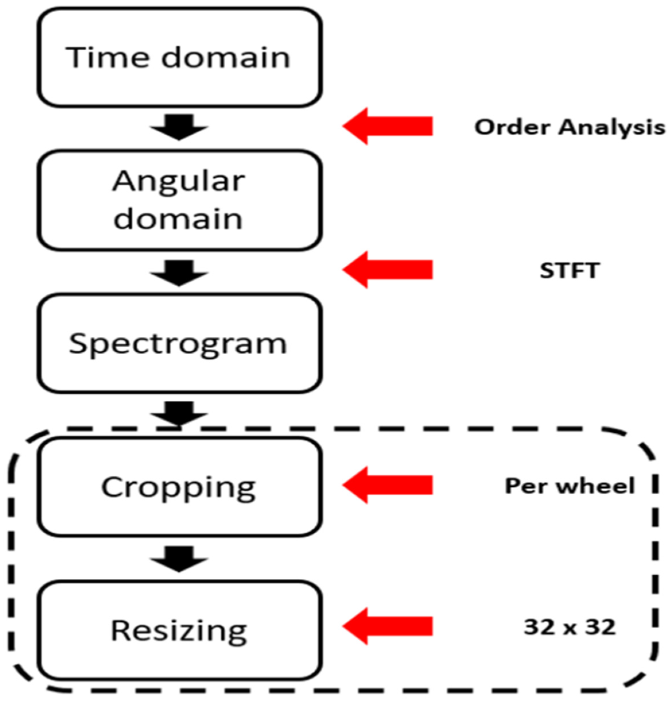
Deep learning results of data with and without signal processing application were compared. In this study, two signal processing methods, order analysis and STFT were used.

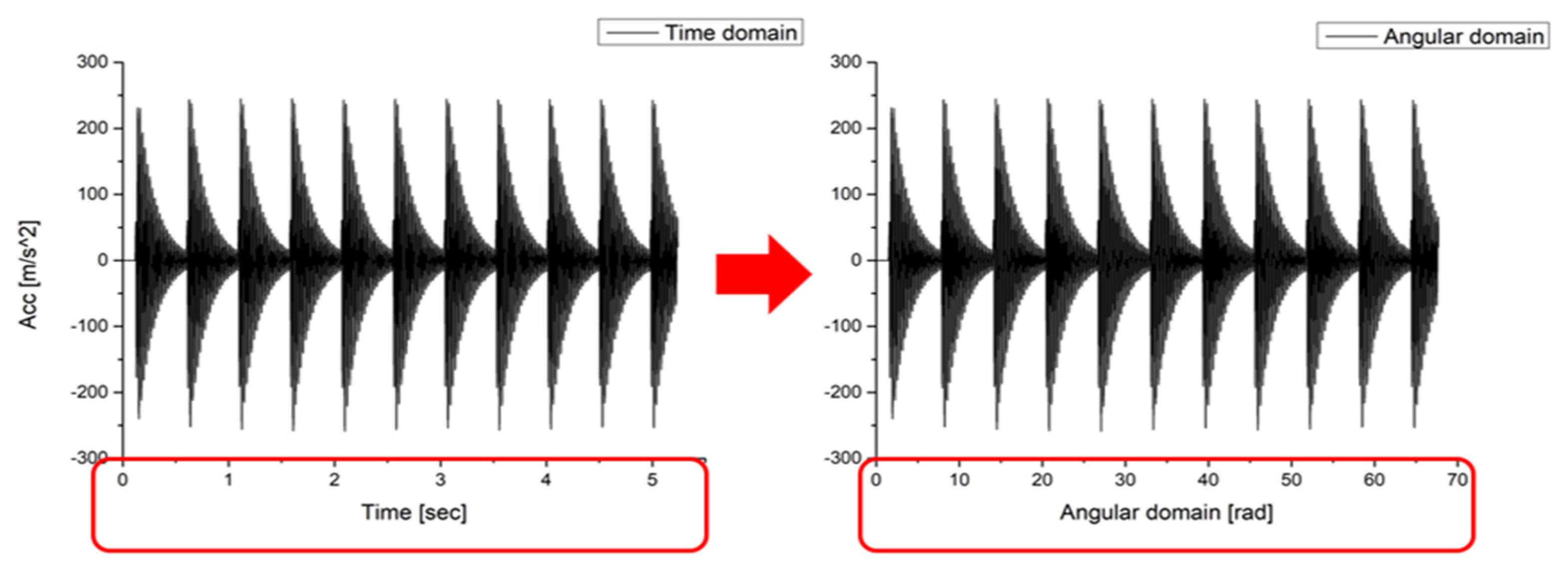
First, order analysis was used in the time domain. In this paper, order analysis is defined as the number of events occurring per unit rotation. Order analysis requires changing the signal to the angular domain before performing FFT of the time domain data [22]. For this reason, order analysis is used to prevent changes in frequency components in a rotating device with varying rotational speeds [23]. Since railway vehicles have various speed changes while driving, it is more useful to convert from the time domain to the angular domain. The tachometer in railway vehicles is always attached to the axle box to measure the rotational speed of the wheelset, which has the advantage of eliminating the need for additional device configuration to convert to the angular domain. 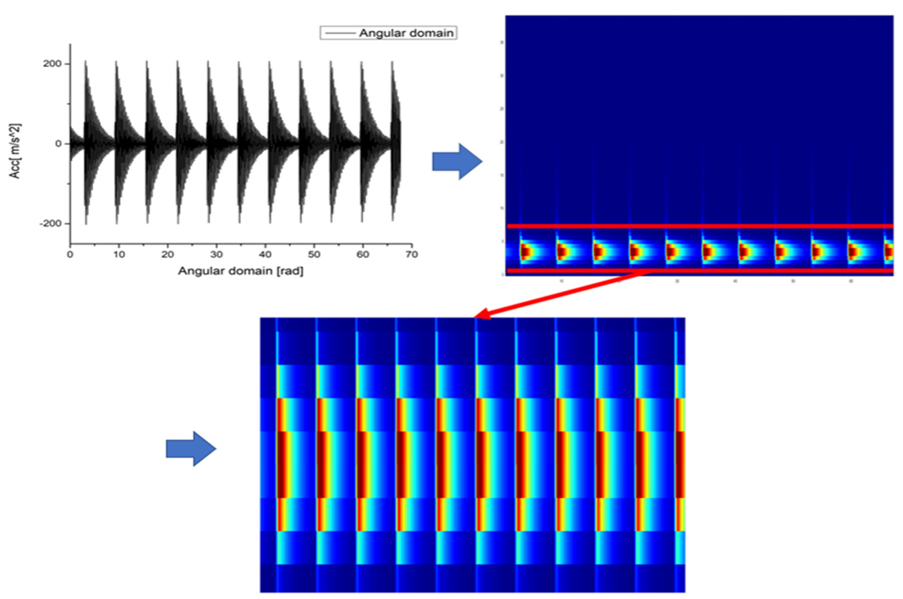Figure 12. shows the conversion of the flat signal from the time domain to an angular domain.

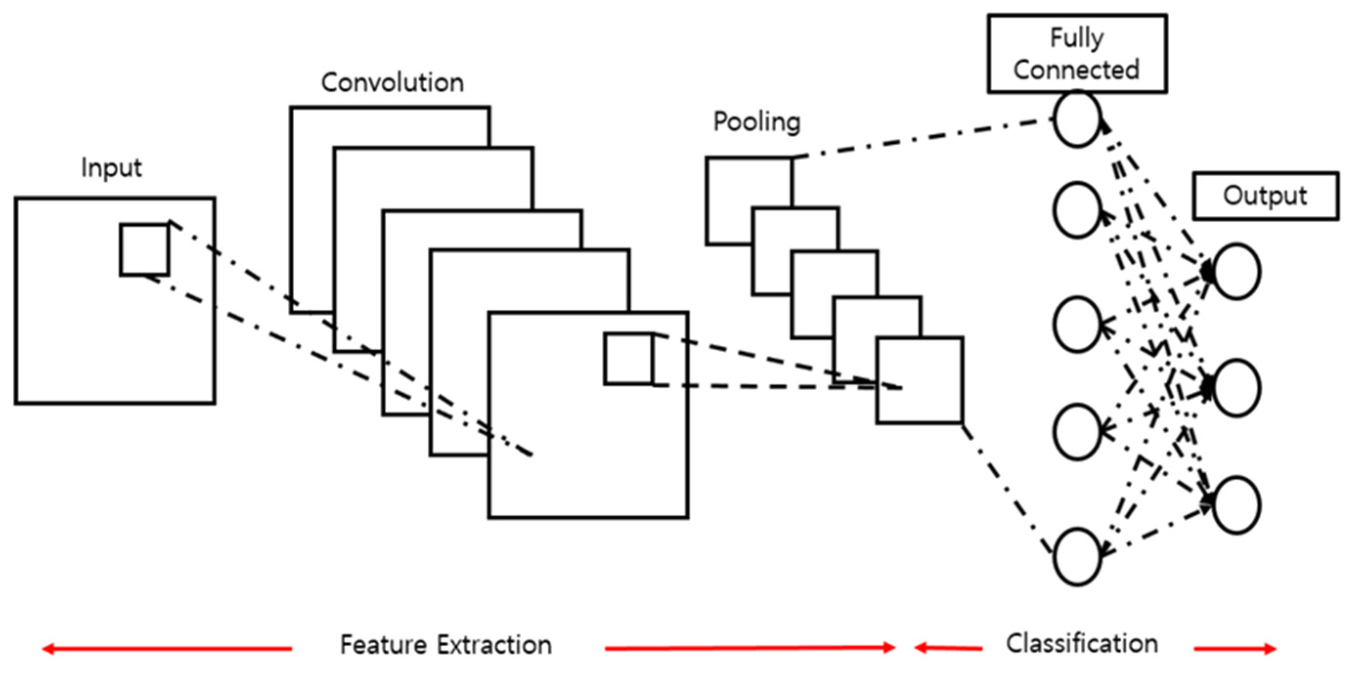
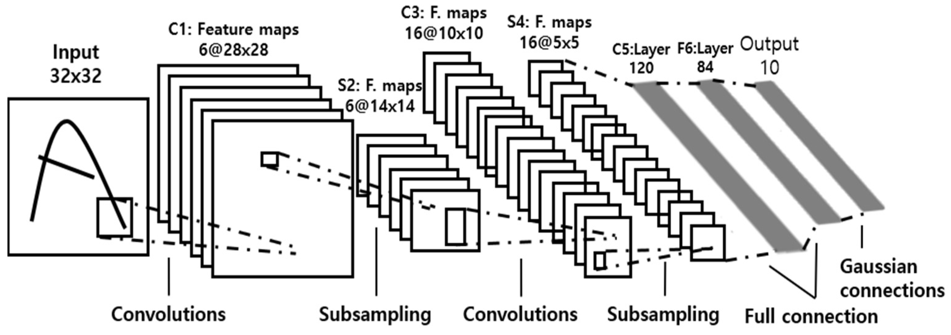
Second, STFT was used since the deep learning algorithm used in this paper is CNN, and CNN is an algorithm suitable for image and video processing, the spectrogram image obtained by STFT was used as learning data.

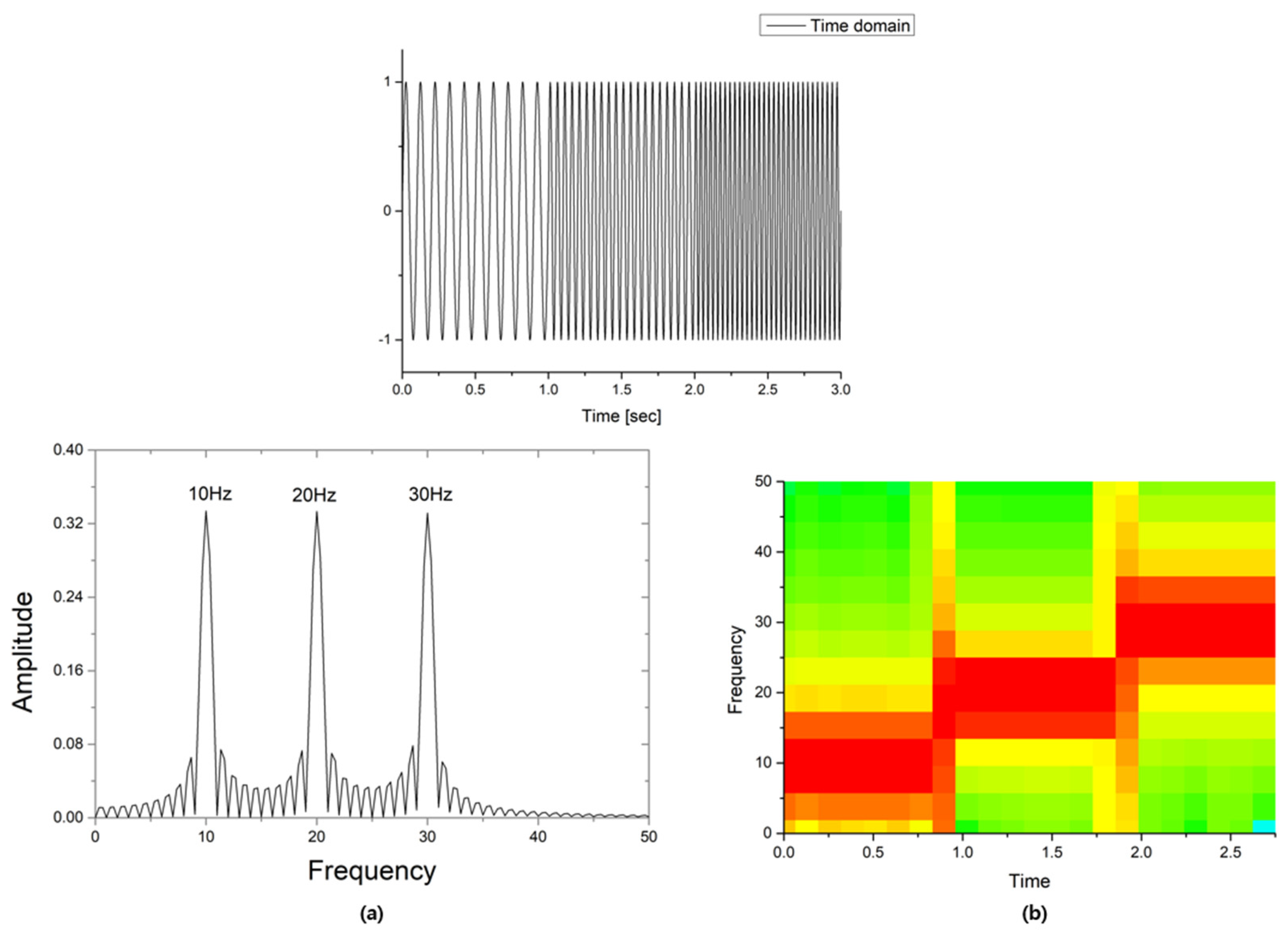
STFT, along with FFT, is one of the most popular analysis methods in the field of noise and vibration analysis [24]. Although the FFT cannot make the frequency change information over time, the STFT can confirm the frequency change information over time by supplementing the disadvantage of the FFT. Figure 13 shows the difference between the STFT and the FFT, where the frequency components of 10 Hz, 20 Hz, and 30 Hz reprinted from ref. [17]. However, as described above, the frequency change according to time elapse could not be visualized through the FFT. This is the second reason for choosing STFT in this paper.

However, there are additional variables to be considered in order to prepare pre-process data that is suitable for deep learning in STFT analysis. First of all, we should consider that the result is different depending on the window function. The analysis results according to the window function were compared. Before comparison, only the frequency band due to wheel flats was set using the Y-Limit function in Matlab, as shown in Figure 14 [25].

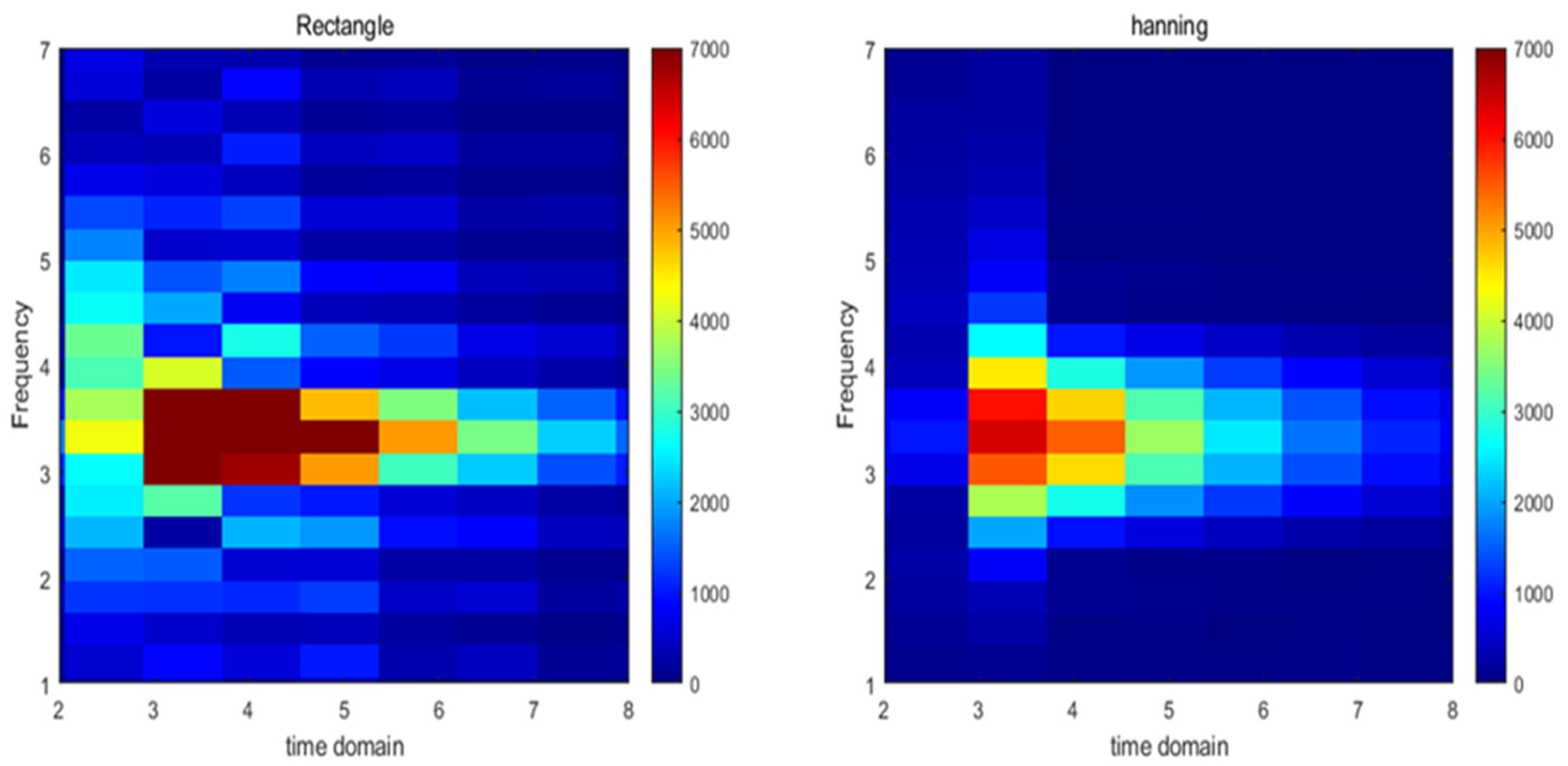
For the window function, both the Rectangular function and Hanning function were compared. At this time, the comparison was made using the data of one flat per wheel. The result is shown in Figure 15. This result shows that the Hanning window is more appropriate because of precise resolution.

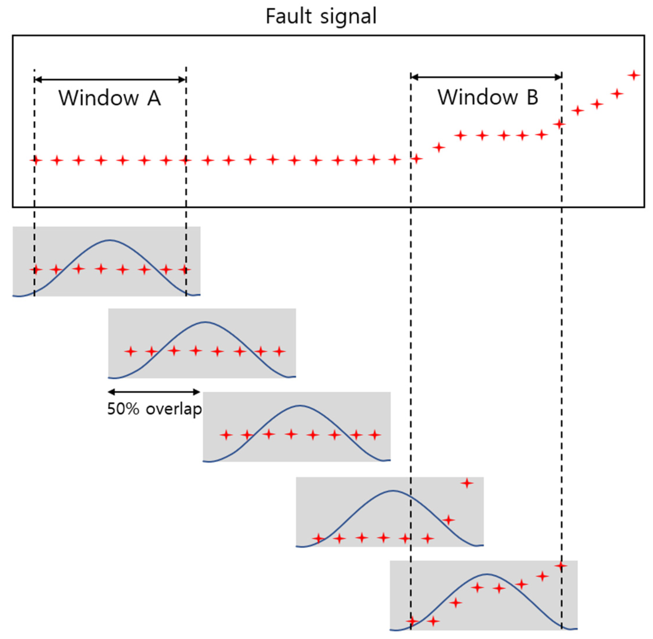
As a second consideration, it is shown that both the frequency and the time resolution vary according to the window length. For example, if the window length is increased, the frequency resolution is improved, but the time resolution degrades. Thus, it should be properly adjusted for the purpose of analysis. However, there is a way to adjust the overlap to alleviate these shortcomings using the concept of overlap shown in Figure 16 [26]. It means that when windows are applied, the windows overlap each other.

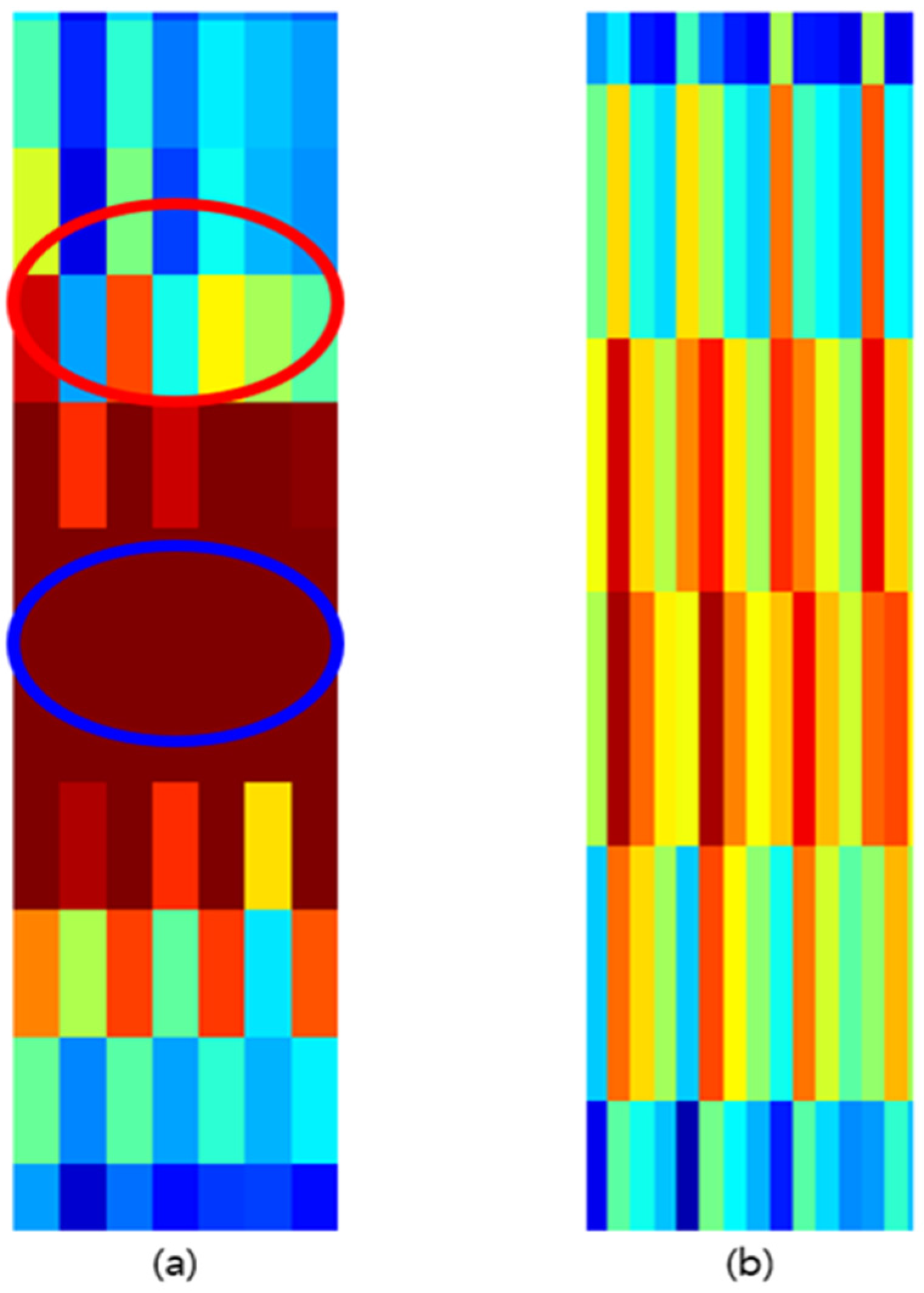
In order to find the window length suitable for this study, the window length was incrementally changed and compared. The data of four wheel flats with window lengths of 128 and 64, respectively, were compared, and the results are shown in Figure 17. As a result of the analysis, it was judged that it was more appropriate to set the window length to 64. For this reason, as shown in Figure 17a, it was not possible to clearly confirm that there were four flat signals in the red and blue circles when compared to (b). Therefore, it was found that as the number of wheel flats increased, the time resolution became more important.

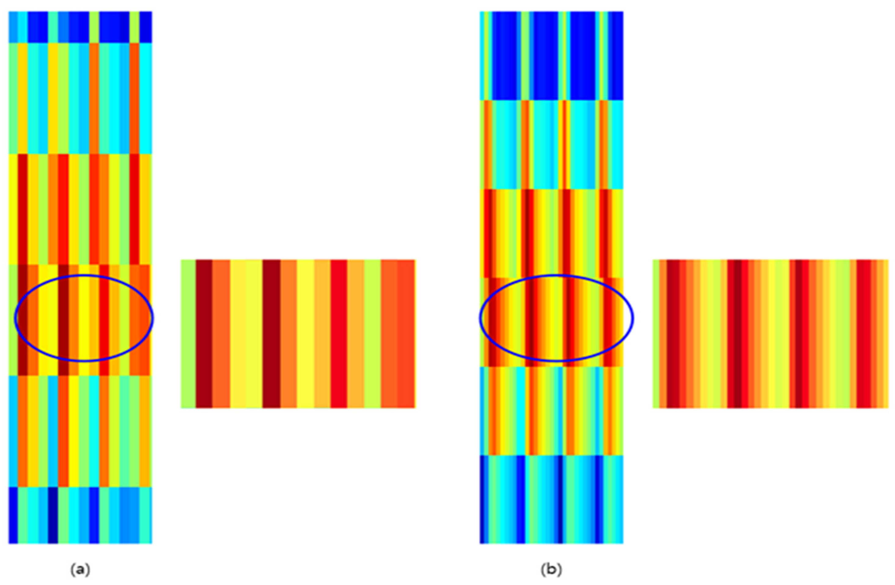
Finally, Figure 18 shows the result of the difference in overlap when the window length is the same as 64. At this time, the cases of overlap 50% and 80% were compared. In addition, the motivation for the comparison with 80% overlap is as follows. First of all, an increase of 10% overlap each from 50% were reviewed. It was confirmed that the case of four wheel flats from 80% overlap is better. Therefore, the cases with 50% and 80% were compared. As a result, it was decided that it is appropriate to set it to 80% as shown in (b) of Figure 18. The reason is that it shows more clearly in four wheel flats in (b) than in (a).

The following parameter values were selected through comparative analysis; First, the window length of 64, the overlap of 80%, and Hanning were used for window function. The final parameter values are summarized in

Table 5. Parameter values of STFT.

Parameter	Value
Window Length	64
Window Function	Hanning
Overlap	80%

, and the final results of applying both order analysis and STFT are shown in Figure 19.

3.2. A Flat Signal Overlapped with a Noise Signal

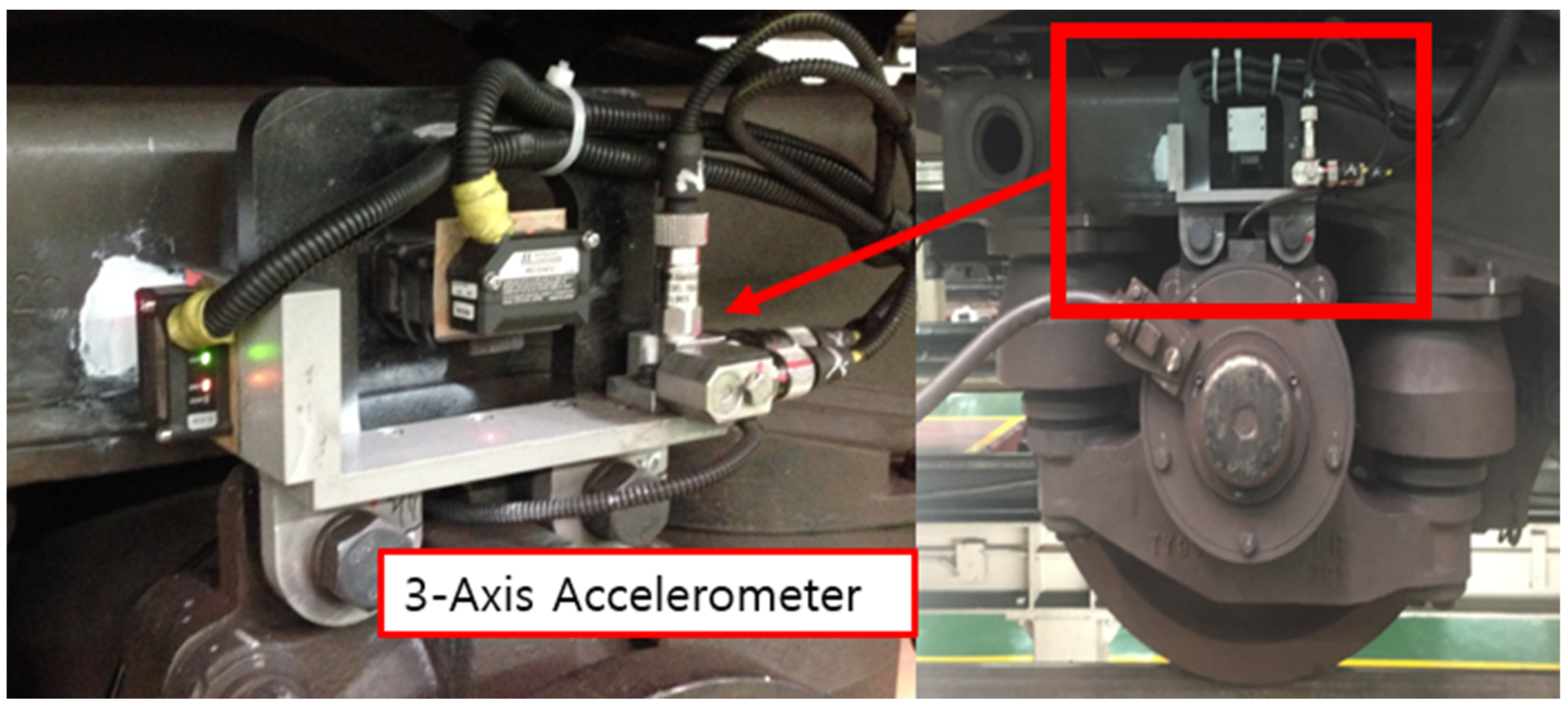
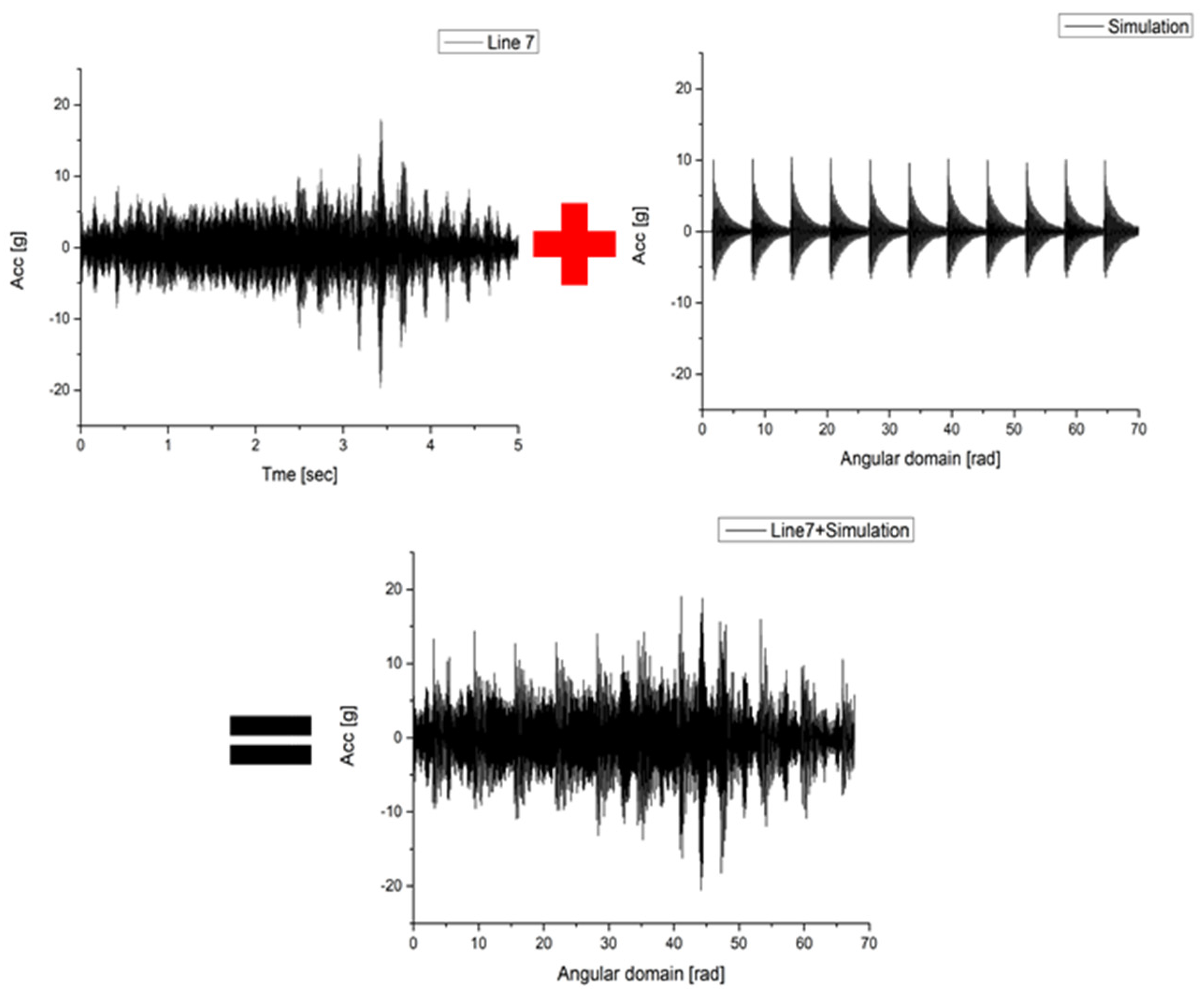
Since it is difficult to obtain data from the driving rail vehicles with wheel flats, the noise signals of normal wheels obtained in past research [17] were overlapped with the simulation flat signals. The noise signals of normal wheels were obtained on the axle box using the Seoul Metro Line 7 vehicle. Figure 20 shows the location of the measuring equipment mounted on the axle box.

Among the overlapped data section, the data of the most severe noise section was applied, and the overlapped result is shown in Figure 21. If the wheel flat size is small, the flat signal (Time-domain) is fully covered by the noise signal. It was found that it is difficult to determine the presence or absence of any small flat signal.

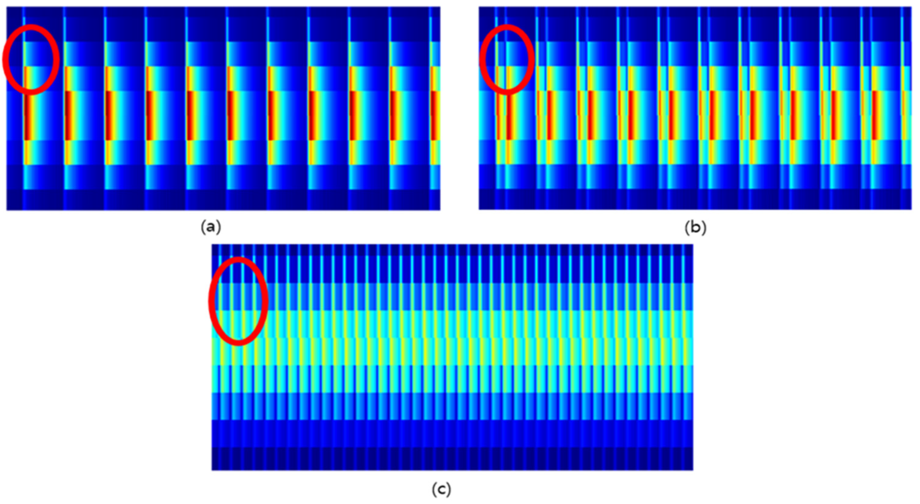
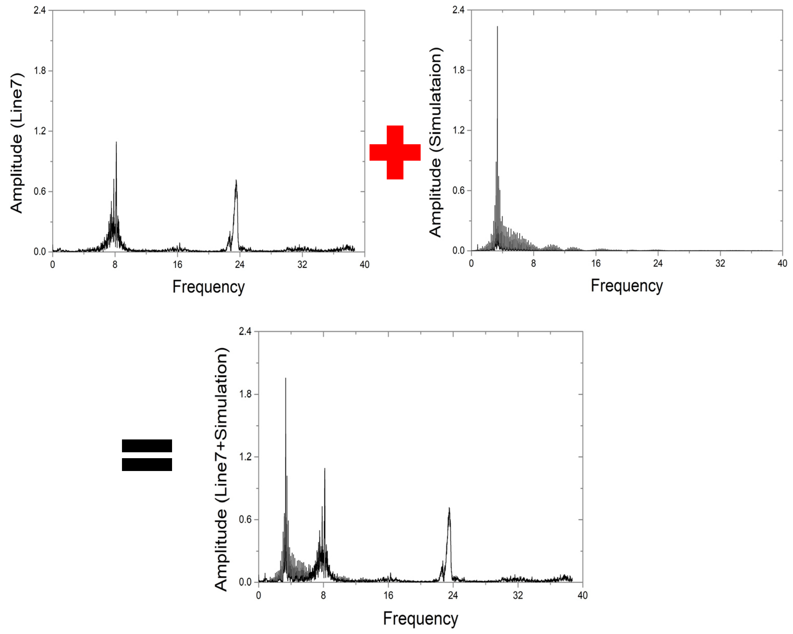
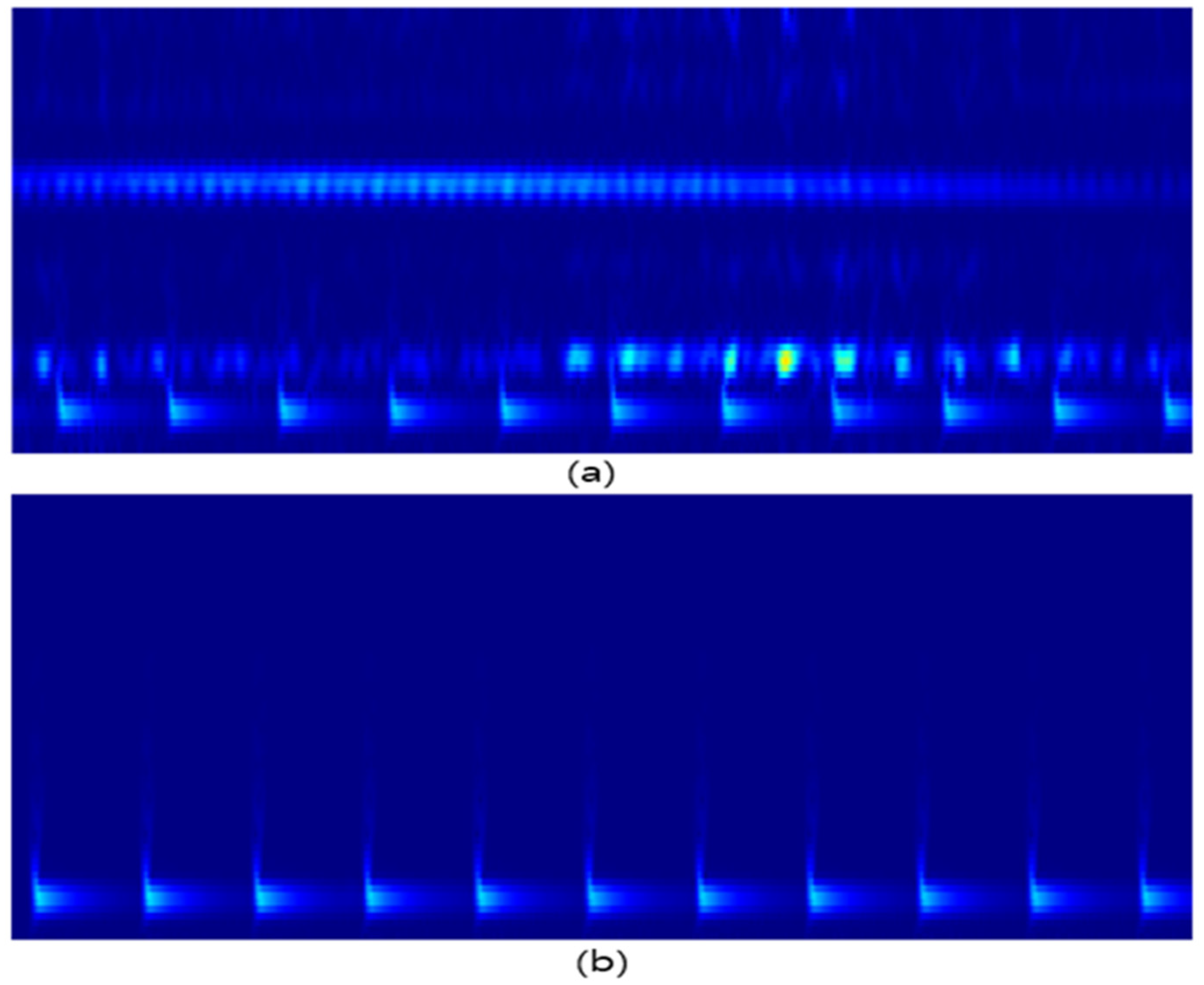
Figure 22 and Figure 23 show the FFT and STFT of the signal overlapped on the noise signal. As a result of the analysis, it was found that the frequency band by the flat signal was relatively low compared to the frequency band by the noise signal, and thus, it was confirmed that the frequency bands are separate from each other.

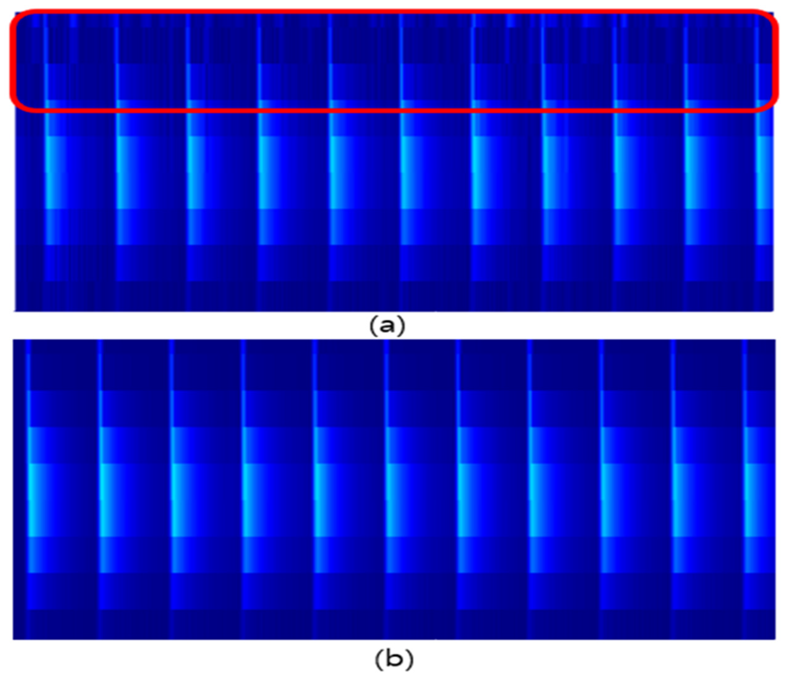
Therefore, as a result of minimizing the influence of the noise signal by cropping only the frequency band indicated by the flats, it was confirmed that only a slight difference appears in the red square shown in Figure 24.

4. Comparison of Deep Learning Results between Signal-Processed Data and No Signal-Processed Data

4.1. CNN (Convolution Neural Network) Algorithm

During deep learning, raw data (Time-domain) was compared with the pre-processed data through signal processing using the CNN algorithm. CNN is a convolution neural network, an algorithm first proposed by Yann LeCun in 1989. The biggest feature is the convolution layer as indicated in the name, and the second feature is the pooling layer, which is also called sub-sampling [27]. Figure 25 shows the basic structure of CNN.

In this paper, the LeNet model was used among CNN algorithms. It was modified to improve performance and speed in the existing architecture, applying modified pooling and activation function. First, the pooling method was changed from the existing average pooling to max pooling. Second, the activation function was changed from the existing Tanh to Leaky ReLu. Finally, Batch Normalization was added. The existing architecture of LeNet-5 is shown in Figure 26 adapted from ref. [28]. In the application of learning, the dataset is usually composed of the ratio of training data, validation data, and test data as 6:2:2 [29]. Therefore, the dataset used in this paper was organized as shown in

Table 6. Dataset is of Training data, Validation data, and Test Data.

Data Type	EA	Ratio [%]
Train Data	2988	60
Validation Data	837	17
Test Data	1152	23

, and the test data was composed of 648 normal data and 504 anomaly data.

Next, a sample of the spectrogram image of normal and anomaly data used for deep learning is shown in Figure 27. The levels of learning were classified into normal and abnormal according to the safety standards for domestic urban railroad vehicles.

As shown in the diagram in Figure 28, the spectrogram image used for learning was resized to 32 × 32 so that it could be fitted in the LeNet model after cropping the image in units of one wheel.

4.2. Deep Learning Results Using the LeNet

When learning the signal processing results, 34 out of 1152 test data could not be accurately determined. Moreover, when learning the raw data results, 308 out of 1152 test data could not be accurately determined. Through this result, the acuity was calculated as shown in Equation (9). The learning time was about 3249 s.

$$\mathrm{Accuracy} =\frac{Number of correct predictions}{Total number of predictions}$$

(9)

As a result of using the LeNet model, signal-processed data had an accuracy of about 97%, whereas raw data without signal processing had an accuracy of about 73.26%. In the case of raw data without signal processing, the reason for the low accuracy was that the flat signal was buried due to the overlap of the raw data (Time-domain) with the noise signal, and thus, the size of the flat was small and the anomaly could not be accurately diagnosed.

In addition to the accuracy, the results of the true positive rate were compared and analyzed through ROC. The ROC curve is frequently used in binary classification models, through which the AUC (Area Under the Curve) value is obtained, and the closer this value is to 1, the higher the reliability is regarded [30]. The result is shown in Figure 29.

Finally, the deep learning results of the preprocessed data through signal processing and the raw data that were not preprocessed are shown in

Table 7. Comparison of deep learning results of STFT and raw data.

Data Type	Accuracy	AUC
STFT	97	0.9688
Raw Data (Time-domain)	73.26	0.7544

. It was confirmed that the result of deep learning with preprocessed data using the signal processing method was about 24% higher in Accuracy and 0.21 in AUC than the result of deep learning based on the Raw data (Time-domain) approach.

5. Conclusions

In this study, an anomaly detection method on the wheel flat problem is proposed. In previous studies, wheel flat is diagnosed using only signal processing techniques without a deep learning approach. This could only detect the presence or absence of a wheel flat. However, in this paper, a deep learning approach is applied to anomaly detection with varying conditions of size and number of wheel flats. At first, the data was pre-processed to be suitable for deep learning through signal processing. Then, anomaly detection was performed using the deep learning technique. The normality and anomaly were classified according to the safety standards of urban railway vehicles. The deep learning model of the LeNet-5 was applied and elaborately modified to observe the performance in a supervised manner for anomaly detection. Different pooling methods and activation functions were applied to improve both the performance and the speed of this domain data.

First, a vibration signal data according to the presence or absence of a wheel flat was obtained using SIMPACK, a multi-body dynamic software. The noise signals measured from Seoul Metro Line 7 were overlapped with the flat signals obtained from the simulations. Then, two signal processing methods were used to create data suitable for deep learning. The wheel of railway vehicles is a rotating device, and its running speed changes frequently during actual operation. Accordingly, as the frequency changes according to the rotation speed, order analysis was performed to compensate for this point. Then, in order to utilize the CNN algorithm during deep learning, a Spectrogram image was created through STFT.

Second, deep learning was performed after changing the LeNet-5 model in the CNN algorithms to improve performance. For the data used in the LeNet model, the size of the spectrogram image was changed to 32 × 32. The deep learning results showed an accuracy of 97%. In addition, the AUC value obtained through the ROC curve, which is often used in the binary classification model, was confirmed. The AUC value was 0.9688, which was also high. Therefore, the anomaly detection technique of wheel flat defects through the LeNet model generated an excellent performance. This study also checked whether the deep learning result was excellent when pre-processing was additionally performed. For this purpose, the raw data (Time domain) was compared with the pre-processing data using the signal processing method. As a result of deep learning, the case with pre-processing was about 24% higher in accuracy, and the AUC value was also about 0.21 higher. The reason is because of noise signal overlapping in the flat signal in the raw data (time-domain) when the wheel flat size was small.

It was well postulated that a study of the anomaly detection for wheel flats with a modified LeNet model would be very meaningful to cultivate further research with deep learning. In addition, it is expected that the following effects will be achieved. First, it is possible to secure the passenger safety and ride comfort of railway vehicles. Second, it is possible to reduce maintenance costs. Third, railway maintenance staff can focus on more important parts of maintenance. This is expected to increase the efficiency of maintenance.

Finally, conducting the tests in real conditions, in the case of rail vehicles, is not so easy in a university laboratory due to safety and cost issues. Because of these reasons, the real flat signal data could not be applied to deep learning. This has been left for future study. Nevertheless, this study would become a useful reference for anomaly detection research on rail vehicles using deep learning. However, this paper first considered the effect of signal processing on the learning sensitivity for anomaly detection of wheel flats. Therefore, for the development of future research, the results will be analyzed through various deep learning models. In addition to the supervised learning method, the semi-supervised method will be used to encourage further research.

References

1. Máté, T.; Zwierczyk, P.T. Finite Element Analysis of Cracks Propagation in Railway Wheels. In Proceedings of the 33rd International ECMS Conference on Modelling and Simulation, Caserta, Italy, 11–14 July 2019; pp. 371–376. [Google Scholar]
2. Ministry of Land, Infrastructure and Transport; Safety Standards for Urban Railway Vehicles, Korea, 2013; Article 43, Table 3. Available online: http://www.molit.go.kr/english/USR/BORD0201/m_28286/DTL.jsp?id=eng_mltm_new&mode=view&idx=2905 (accessed on 16 November 2022).
3. Lee, K.S.; Kim, J.W. A Study on Strategy of Condition Based Maintenance for Rolling Stock. J. Korean Soc. Railw. Korea 2015, 391–395. [Google Scholar]
4. Hyundai Rotem; Responsible for Safety and Operational Efficiency with Smart Technology, Hyundai Rotem’s Health-Based Maintenance (CBM) System. Korea. 2021. Available online: https://tech.hyundai-rotem.com/digital/cbm-overview/ (accessed on 5 October 2022).
5. Kim, G.; Kim, H.; Koo, J. A Study on Cepstrum Analysis for Wheel Flat Detection in Railway Vehicles. J. Korean Soc. Saf. 2016, 31, 28–33. (In Korea) [Google Scholar] [CrossRef] [Green Version]
6. Park, B.; Lee, Y.; Lee, C. Tool Condition Monitoring Using Deep Learning in Machining Process. J. Korean Soc. Precis. Eng. 2020, 37, 415–420. (In Korea) [Google Scholar] [CrossRef]
7. Randall, R.B. State of the Art in Monitoring Rotating Machinery. Sound Vib. 2004, 38, 14–21. [Google Scholar]
8. Gao, R.; He, Q.; Feng, Q. Railway Wheel Flat Detection System Based on a Parallelogram Mechanism. Sensors 2019, 19, 3614. [Google Scholar] [CrossRef] [PubMed] [Green Version]
9. Liang, B.; Iwnicki, S.; Feng, G.; Ball, A.; Tran, V.T.; Cattley, R. Railway Wheel Flat and Rail Surface Defect Detection by Time-frequency Analysis. Chem. Eng. Trans. 2013, 33, 745–750. [Google Scholar]
10. Yang, C.; Sun, Y.; Ladubec, C.; Liu, Y. Developing Machine Learning-Based Models for Railway Inspection. Appl. Sci. 2021, 11, 13. [Google Scholar] [CrossRef]
11. Chandran, P.; Thiery, F.; Odelius, J.; Lind, H.; Rantatalo, M. Unsupervised Machine Learning for Missing Clamp Detection from an In-Service Train Using Differential Eddy Current Sensor. Sustainability 2022, 14, 1035. [Google Scholar] [CrossRef]
12. Chandran, P.; Thierry, F.; Odelius, J.; Famurewa, S.M.; Lind, H.; Rantatalo, M. Supervised Machine Learning Approach for Detecting Missing Clamps in Rail Fastening System from Differential Eddy Current Measurements. Appl. Sci. 2021, 11, 4018. [Google Scholar] [CrossRef]
13. Yokouchi, T.; Kondo, M. LSTM-based Anomaly Detection for Railway Vehicle Air-Conditioning Unit using Monitoring Data. In Proceedings of the IECON 2021–47th Annual Conference of the IEEE Industrial Electronics Society, Toronto, ON, Canada, 13–16 October 2021; pp. 1–6. [Google Scholar]
14. Jahan, K.; Umesh, J.P.; Roth, M. Anomaly Detection on the Rail Lines Using Semantic Segmentation and Self-Supervised Learning. In Proceedings of the 2021 IEEE Symposium Series on Computational Intelligence (SSCI), Orlando, FL, USA, 5–7 December 2021; pp. 1–7.
15. Bosso, N.; Gugliotta, A.; Zampieri, N. Wheel flat detection algorithm for onboard diagnostic. Measurement 2018, 123, 193–202. [Google Scholar] [CrossRef]
16. Brizuela, J.; Fritsch, C.; Ibáñez, A. Railway wheel-flat detection and measurement by ultrasound. Transp. Res. Part C Emerg. Technol. 2011, 19, 975–984. [Google Scholar] [CrossRef]
17. Shim, J.S. A Study on the Anomaly Detection of Wheel Flat Using Deep Learning Techniques. Ph.D. Thesis, Seoul National University of Science and Technology, Seoul, Korea, 2022. [Google Scholar]
18. Dassault System, SIMPACK User Assistant 2020x4: Vélizy-Villacoublay, France, 2020.
19. Bian, J.; Gu, Y.; Murray, M.H. A dynamic wheel–rail impact analysis of railway track under wheel flat by finite element analysis. Veh. Syst. Dyn. 2012, 51, 784–797. [Google Scholar] [CrossRef] [Green Version]
20. Shim, J.; Kim, G.; Cho, B.; Koo, J. Application of Vibration Signal Processing Methods to Detect and Diagnose Wheel Flats in Railway Vehicles. Appl. Sci. 2021, 11, 2151. [Google Scholar] [CrossRef]
21. Li, Z.; Molodova, M.; Núñez, A.; Dollevoet, R. Improvements in Axle Box Acceleration Measurements for the Detection of Light Squats in Railway Infrastructure. IEEE Trans. Ind. Electron. 2015, 62, 4385–4397. [Google Scholar] [CrossRef]
22. Kim, K.Y. A Study on the Vibration Signal Processing Method for Wheel Flat Detection and Diagnosis in Railway Vehicles. Ph.D. Thesis, Seoul National University of Science and Technology, Seoul, Korea, 2016. [Google Scholar]
23. Yang, W.S.; Lee, W.P.; Lee, J.W. Development of Inspection Methods for Bearing Faults with a Rapid Change of Rotation Speed and Optimization of Pass/Fail Criteria. Trans. Korean Soc. Automot. Eng. 2017, 25, 273–286. [Google Scholar] [CrossRef]
24. Jeon, H.; Jung, Y.; Lee, S.; Jung, Y. Area-Efficient Short-Time Fourier Transform Processor for Time–Frequency Analysis of Non-Stationary Signals. Appl. Sci. 2020, 10, 7208. [Google Scholar] [CrossRef]
25. Matlab Help R2021a; MathWorks: Natick, MA, USA, 2021.
26. Yeap, Y.M.; Ukil, A.; Geddada, N. STFT Analysis of High Frequency Components in Transient Signals in Multi-Terminal HVDC System. In Proceedings of the IECON 2016-42nd Annual Conference of the IEEE Industrial Electronics Society, Florence, Italy, 23–26 October 2016; pp. 4008–4013. [Google Scholar]
27. WIKIPEDIA. CNN Convolutional Neural Network. Last Edited on 3 October 2022, at 10:13 (UTC). Available online: https://en.wikipedia.org/wiki/Convolutional_neural_network (accessed on 5 October 2022).
28. LeCun, Y.; Bottou, L.; Bengio, Y.; Haffner, P. Gradient-based learning applied to document recognition. Proc. IEEE 1998, 86, 2278–2324. [Google Scholar] [CrossRef] [Green Version]
29. Yoon, H.J. Finding Unexpected Test Accuracy by Cross Validation in Machine Learning. IJCSNS Int. J. Comput. Sci. Netw. Secur. 2021, 21, 549–555. [Google Scholar]
30. Cho, H.; Matthews, G.J.; Harel, O. Confidence Intervals for the Area Under the Receiver Operating Characteristic Curve in the Presence of Ignorable Missing Data. Int. Stat. Rev. 2019, 87, 152–177. [Google Scholar] [CrossRef] [PubMed]
Figure 1. Wheel Flat.
Applsci 12 12901 g001
Figure 2. Railway vehicles modeling.
Applsci 12 12901 g002
Figure 3. Bogie modeling.
Applsci 12 12901 g003
Figure 4. The location of the wheel flat.
Applsci 12 12901 g004
Figure 5. Coordinate values using Acro Edit.
Applsci 12 12901 g005
Figure 6. Wheel configuration for calculating coordinates.
Applsci 12 12901 g006
Figure 7. Modeling manual for wheel flat in SIMPACK [18].
Applsci 12 12901 g007
Figure 8. Dz-Wheel raised in the SIMPACK post result.
Applsci 12 12901 g008
Figure 9. Principle of wheel and rail collision by wheel flat [19].
Applsci 12 12901 g009
Figure 10. Acceleration signals of x, y, and z axis due to wheel flat impact against rail.
Applsci 12 12901 g010
Figure 11. Schematic of the instrumentation setup for wheel flat measurements [21].
Applsci 12 12901 g011
Figure 12. Conversion of the flat signal from the time domain to an angular domain.
Applsci 12 12901 g012
Figure 13. Difference between (a): FFT and (b): STFT [17].
Applsci 12 12901 g013
Figure 14. Frequency band due to wheel flats.
Applsci 12 12901 g014
Figure 15. Comparison of Rectangular function and Hanning function.
Applsci 12 12901 g015
Figure 16. Definition of overlap [24].
Applsci 12 12901 g016
Figure 17. Comparison of (a): window length 128 and (b): window length 64.
Applsci 12 12901 g017
Figure 18. Comparison of (a): overlap 50% and (b): overlap 80%.
Applsci 12 12901 g018
Figure 19. Final results of applying both order analysis and STFT [(a): flat 1ea, (b): flat 2ea, (c): flat 4ea].
Applsci 12 12901 g019
Figure 20. Location of the measuring equipment mounted on the axle box.
Applsci 12 12901 g020
Figure 21. Overlap result (Time domain).
Applsci 12 12901 g021
Figure 22. FFT of the signal overlapped on the noise signal.
Applsci 12 12901 g022
Figure 23. STFT of the signal overlapped on the noise signal [(a): with noise, (b): without noise].
Applsci 12 12901 g023
Figure 24. Difference between with noise signals and without noise signals in STFT [(a): with noise, (b): without noise].
Applsci 12 12901 g024
Figure 25. Architecture of CNN.
Applsci 12 12901 g025
Figure 26. Architecture of LeNet-5 [28].
Applsci 12 12901 g026
Figure 27. Samples of normal and abnormal data.
Applsci 12 12901 g027
Figure 28. Pre-process diagram using a signal processing method.
Applsci 12 12901 g028
Figure 29. Comparison of AUC value of STFT and raw data (Time-domain).
Applsci 12 12901 g029