Article

A Modeling Approach for Measuring the Performance of a Human-AI Collaborative Process

1
School of Engineering, Computing and Mathematics, University of Plymouth, Plymouth PL4 8AA, UK
2
Business Information Systems, Hochschule Furtwangen University, 78120 Furtwangen, Germany
*
Authors to whom correspondence should be addressed.
Appl. Sci. 2022, 12(22), 11642; https://doi.org/10.3390/app122211642
Submission received: 14 October 2022 / Revised: 7 November 2022 / Accepted: 12 November 2022 / Published: 16 November 2022
(This article belongs to the Special Issue Artificial Intelligence in Complex Networks)

Abstract

:
Despite the unabated growth of algorithmic decision-making in organizations, there is a growing consensus that numerous situations will continue to require humans in the loop. However, the blending of a formal machine and bounded human rationality also amplifies the risk of what is known as local rationality. Therefore, it is crucial, especially in a data-abundant environment that characterizes algorithmic decision-making, to devise means to assess performance holistically. In this paper, we propose a simulation-based model to address the current lack of research on quantifying algorithmic interventions in a broader organizational context. Our approach allows the combining of causal modeling and data science algorithms to represent decision settings involving a mix of machine and human rationality to measure performance. As a testbed, we consider the case of a fictitious company trying to improve its forecasting process with the help of a machine learning approach. The example demonstrates that a myopic assessment obscures problems that only a broader framing reveals. It highlights the value of a systems view since the effects of the interplay between human and algorithmic decisions can be largely unintuitive. Such a simulation-based approach can be an effective tool in efforts to delineate roles for humans and algorithms in hybrid contexts.

1. Introduction

The phenomenal growth of AI in recent years, especially machine learning (ML), a self-improving subfield of AI, has cemented its status as a general-purpose technology [1], like the steam engine or electricity of the past. Therefore, and unsurprisingly, it is also at the center of a strident debate about its impact across multiple dimensions (e.g., economic, social, and ethical) [2], with two very noticeable camps emerging: the optimists and the pessimists [3]. The former camp primarily extolls the virtues (current or anticipated) of ML benefiting all of humanity. The latter, however, warns us about technological sophistication outstripping our ability to reason about its unintended consequences.
Less noticeable, but increasingly gaining traction, is a third camp composed of pragmatists. While acknowledging AI’s staggering achievements (thus refuting ardent pessimists), they point out that much progress is still ahead of us and call attention to mounting evidence that should give pause to unchecked optimism. In this view, numerous examples of brittleness (for instance, in the face of adversarial ML) [4,5], poor out-of-distribution performance [6], challenges with explainability [7] (compounded by regulatory pressures [8]), and poor adoption [9] must count as evidence. (On the last point, a recent study has shown that the adoption rate of AI in organizations in the US is less than 7% [10].)
Pragmatism about ML’s status and prospects promotes recognition that autonomy is not a viable goal in numerous situations, particularly in open-ended problems (where there is uncertainty about relevant variables, and the effects of causes tend to be distant in space and time). It leads to advocacy for humans in the loop [11]. Of course, given the field’s dynamism, the nature of human–ML collaboration must naturally evolve, as well. Therefore, the inevitability of roles for humans in complex decision-making situations coupled with the fast-paced nature of technological change elicits a nuanced view of automation. On this account, a picture of automation antithetical to a simplistic either/or dichotomy [12] emerges.
It is a picture of persistent tension caused by task interdependencies, which are apt to change over time, giving rise to spatial and temporal dynamism. For example, Shestakofsky’s [13] empirical work shows that automating a task impacts adjacent tasks in that these (say, previously manual tasks) might benefit from augmentation. Furthermore, the trajectory of these changes heavily depends on the organizational context. Therefore, what further crystallizes is an argument that rejects technological determinism [14] and places importance on context. One where besides the apparent technical aspects, gross behavioral elements such as social relations and politics play substantial roles—a view that accords with the economic theory of complementarities [15]. It holds that studying technological adoption benefits from viewing the human–technology ensemble as a sociotechnical system embedded in an organization, creating a system of complements, a more formal notion of the intuitive idea of synergy.
Although the literature on complementarity illuminates how organizational value derives from the interactions between the embedded technology and the surrounding organizational and broader environmental factors [16], there is a gap when the technology in question is ML [17]. The autonomy that ML affords, albeit partial, represents a break from traditional IT that predominates the discourse about the impact of technology on value creation and capture. In particular, ML’s role transcends a mere tool and can assume various other roles, such as those of assistant, peer, and manager [18], depending on context/maturity [19]. A profound consequence of this, plainly stated, is that the ML agents (the technology) now contribute to organizational learning, the object of which is organizational mental models that drive behavior (and create value, or not). Puranam [20] points out an unprecedented dynamic in the history of the technology-driven complementarities that this produces. ML agents can now make the same decisions as humans. So, through aggregation (the wisdom of crowds effect [21]), organizations could generate performance superior to what humans or ML can achieve working alone. Since organizational mental models are the storehouse of creativity, this further implies that, jointly, not just improving existing ways but entirely new ways of doing things (the realm of strategy) open up [22].
The modest premises discussed (self-learning ML, the importance of humans in the loop, and new forms of complementarity that ML affords) combine to yield enormous implications for organizational performance. The challenge of achieving the desired level of performance transforms into a coordinating coalition of human and ML agents that explore the performance landscape in search of tall peaks. Since in the real world of organizational problem-solving, payoffs and the menu of choices are uncertain [23] (as opposed to the closed world of games)—what Hogarth terms “wicked” problems [24]—the exploration has to contend with a “rugged landscape” [25] (i.e., the risk of local maxima).
Knudsen and Srikanth [26] observe that prior work on the normative question of exploring the terrain—or the problem space [27]—in search of satisfactory solutions assumes the organization as a “unitary actor”. They note that researchers have scarcely attended to the collaborative aspects (in particular, the role of mutual learning). For instance, the issue of second-guessing arises when there are multiple agents, which can lead to dysfunctional behavior such as, to use their phrasing, “joint myopia” (or local rationality [28]) or “mutual confusion” (a result of misperceiving the causes of positive or negative payoffs). Although further complexities arise when humans and ML team up [17], a standout dimension is the inability of ML to fully imbibe tacit knowledge [29] that is crucial to solving many complex tasks.
This is a topic that opens up several avenues for research. However, they fall into two broad categories. The first is research that focuses on the usability aspects of the technology itself. For instance, a burgeoning field known as explanatory AI [30] tries to make ML models less opaque by endowing them with the ability to answer “why” questions, that is, why a specific result or counterfactual questions such as “what would have happened had the input been different?” (in short, an ability to “introspect” their “beliefs”). The second concerns itself with the appropriate use of ML to maximize value—organizational design questions such as the division of labor between humans and ML, and ideal learning configurations [20] fall in this category.
A prerequisite to fruitful research pursuit in either category is the ability to evaluate the combined rationality [31] sufficiently broadly to elucidate the contribution of ML (and, by extension, data) in the context of a longer means-end chain (connecting behavior to business value). It is to this that our work seeks to contribute. We adopt a simulation-based approach (using system dynamics) for the evaluation model. System dynamics is particularly amenable to investigating emergent properties of interdependent actions since it emphasizes dynamic complexity [32] (e.g., due to feedback, a core component of learning) more than component-level complexity. Specifically, our contributions are two-fold:
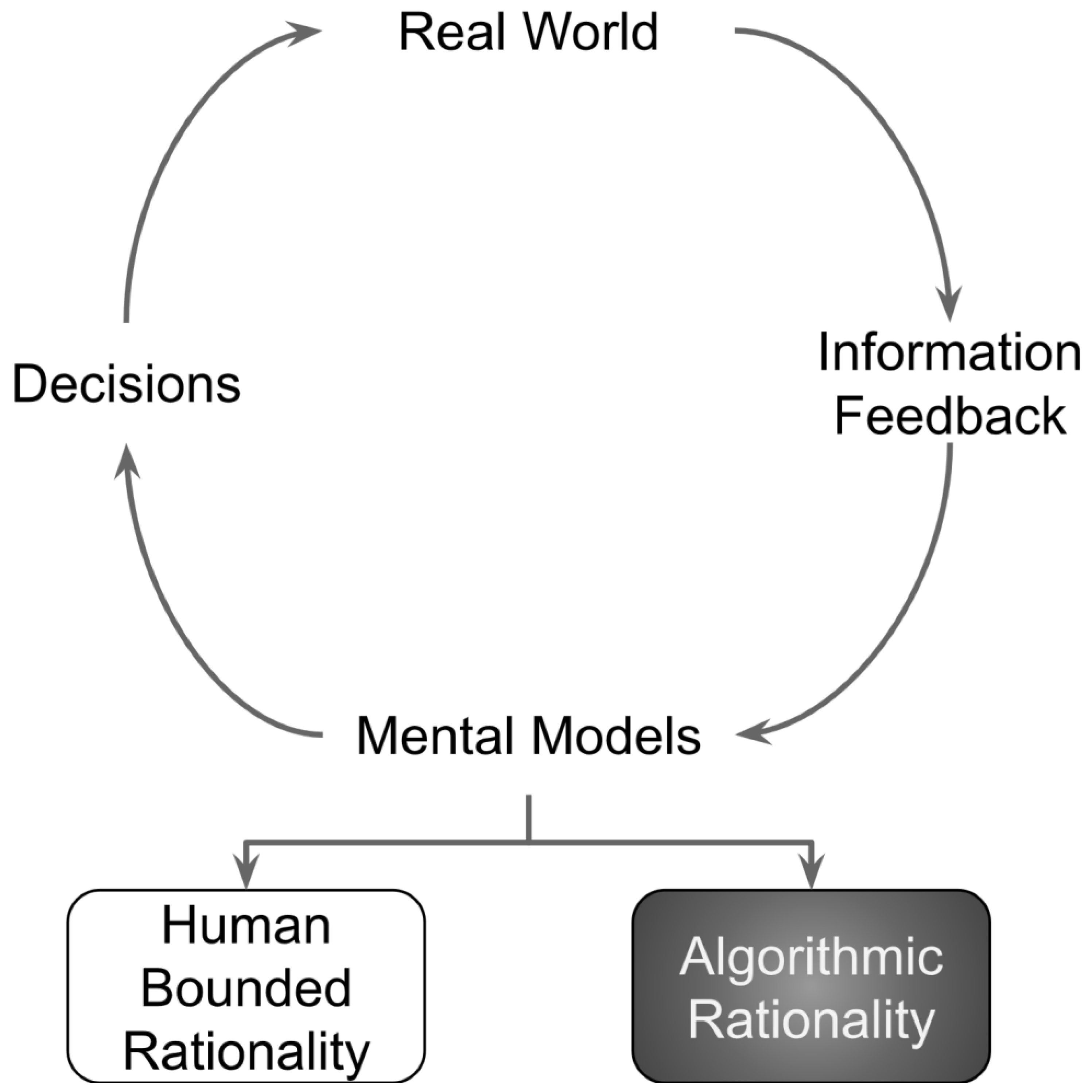
  • We complement the conceptual literature on human–ML teaming that, by necessity (as it caters to various types of organizations), provides general guidelines on effectively structuring collaborations. Our modeling framework allows quantification of the blending of algorithmic ML rationality and bounded human rationality. We test our approach using an imaginary case of a company trying to improve its supply chain planning process.
  • We complement existing work on explanatory AI in terms of framing “why” questions. Concretely, two metrics generally evaluate ML’s explanations: interpretability and completeness [33]. Our model provides the organizational problem-solving context (shedding light on the landscape of choices human and ML agents navigate) that must inform the selection of relevant “why” questions.
The structure of the remainder of the paper is as follows. In Section 2, we discuss conceptual frameworks that provide guidelines for human–ML role separation, from which we draw insights that inform the theoretical base for the quantitative framework. In Section 3, we justify our design choices in the framework. Specifically, we explain why choosing a systems approach to modeling best fits the design requirements outlined at the end of Section 2. In Section 4, we describe the details of the framework and run tests using synthetic data to validate our central claim about the risk of local rationality. Finally, in Section 5, we discuss the implications of our findings and comment on what they have to say about related work in this area.

2. Related Work

Various qualitative approaches in the literature suggesting the creation of a human–ML coalition adopt as a guide the insight that ML suffers from what Marcus terms “pointillistic” intelligence [6]. Therefore, in this reading, the overarching brief for humans is to serve as orchestrators in the group such that it can exhibit “general collective intelligence” [18]; Malone describes this group of human strategists and ML tacticians as superminds. Kasparov has written about the strategy/tactics distinction [34] in the context of chess, which serves as a valuable proxy for any intellectual endeavor [35]. It stems from acknowledging that although the cognitive architecture of humans predisposes them to poor performance (compared to ML) on memory and information processing, it allows them to excel in long-term planning, crucial for convergent thinking or the process that results in choosing from among alternatives. (The importance of strategy to decision-making is why Malone recommends that we consider putting computers in the group rather than putting humans in the loop as the mantra for creating effective coalitions.)
Despite the heterogeneity in the details informed by diverse philosophical and intellectual commitments, these approaches share a similar strategy for delineating human and ML roles. They rely on noticing that tasks, seen through the lens of tractability, fall along a spectrum, with some resembling games—fictions of the human mind—or are “game-like”, while others, closer to life itself, are “life-like”. Game-like tasks are more agreeable to a closed formulation as they have more of the following properties. The rules are well specified and require minimal background knowledge, feedback is unambiguous, feedback loops are short, and behavior is observable. From the perspective of objective attainment, such properties contribute to the connections between the means and the end being neither tenuous nor uncertain (unlike in life-like tasks where the structure is a “tangled web” [36]). It also implies much less difficulty in agreeing on the “best” means for a given end, further aiding a closed formulation.
In contrast, several factors complicate modeling efforts for life-like tasks where social aspects dominate, the value-ladenness of means/ends scuttles efforts to find the “best” option, and poor or absent feedback contributes to flawed mental models. In short, game-like tasks represent a “kind” environment, whereas life-like tasks inhabit a “wicked” environment [24]. A sensible strategy that the approaches often adopt is carefully choosing dimensions that allow the ordering of tasks along the game-like/life-like spectrum, suggesting the appropriate blending of algorithmic and human rationality. In this way, the dimensions proposed include open/closed [19], weak/severe (according to risk) [19], social/asocial [37], creativity/optimization [37], low-dexterity/high-dexterity [37], decision space specificity, size, decision-making transparency, speed, and reproducibility [21], abstraction, intuition/prediction, simulation [38], and thinking/feeling [39].
Although the conceptual models provide a means to assess tasks according to their suitability for ML, they suffer from a critical drawback. Since the recommendations must be broadly applicable, the frameworks have an “objective” bias regarding the problem (that human–ML teams must solve), which yields a disinterested observer or experimenter’s eye view of the problem. However, one can scarcely begin to solve real-world problems as posed. A wealth of research in cognitive science supports the importance of framing or problem representation, emphasizing the complexity reduction aspects of problem-solving that make otherwise intractable problems solvable. In their seminal paper on human problem solving, Newell and Simon [27] draw a distinction between the objective problem, the “task environment”, in their phrasing, and the problem representation (namely, the “problem space”). The transformation process from the former to the latter is a function of problem complexity. Most problems of interest in organizational decision-making—the consumers of the conceptual frameworks—elude optimal solutions requiring significant simplification efforts. (Simon introduced the term “satisficing” to denote the finding of inexact but satisfactory solutions [40].)
The contrast between the (unreasonable) expectations of optimally solving problems and the reality of searching for a suitable representation that yields good-enough solutions mirrors the contrasting philosophies of the economic man and bounded rationality in cognitive psychology. Several streams of research in organizational theory have explored the implications of bounded rationality in decision-making. They include Klein’s naturalistic decision-making [41], Galbraith’s organizational information-processing theory [42], Nelson and Winter’s evolutionary theory of economic change [43], and Gigerenzer’s ecological rationality [44]. These efforts outline structures and tactics that constitute organizational adaptations to the challenges of their task environments. In unison, they reject the idea of an infinitely malleable organization that takes the shape of the problem it is trying to solve, thereby advocating subjectivity (that bounded rationality inevitably entails).
Among the concepts that underpin problem-simplification approaches, the notion of hierarchy stands out as a unifying construct serving as a conceptual glue—in Simon’s words, “[h]ierarchy […] is one of the central structural schemes that the architect of complexity uses” [40]. Hierarchy captures the essence of the near-universal technique of breaking down a complex problem into simpler parts that complex systems embrace. The concept of hierarchical planning systems [45], widespread in supply chain management, vividly illustrates the divide-and-conquer approach inherent in the hierarchical notion. In hierarchical planning’s most straightforward formulation, the system stratifies decisions into strategic, tactical, and operational. As a problem passes through the stages, it undergoes the progressive addition of constraints that transform a relatively open problem into a closed one. It results in the sequential imbuing of subjectivity, simultaneously simplifying and providing context to the problem for the organization.
The preceding discussion highlights the importance of an organization-specific problem formulation for evaluating the pairing of humans and ML.
Since such an evaluation typically precedes implementation, it must be quantitative and, given that organizational decisions are context-rich, sufficiently broad in scope, enabling a holistic assessment. To the best of our knowledge, such a quantitative simulation-based model to evaluate the blending of formal/ML and substantive/human rationality in a holistic context is currently lacking, a gap this paper seeks to redress.

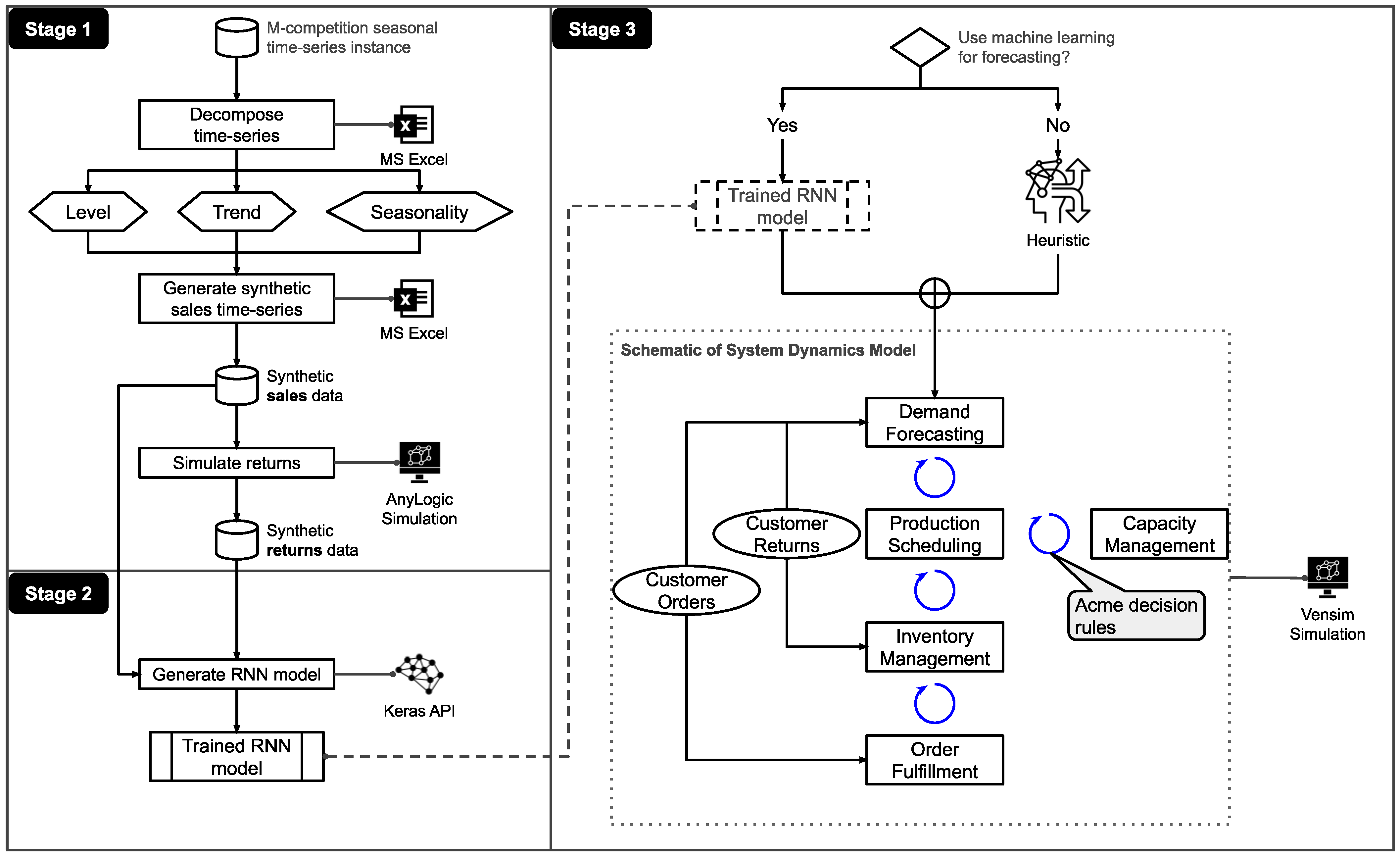
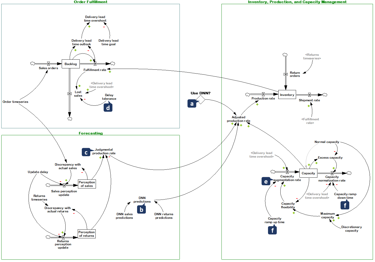
3. Design of a Quantitative Model

The desirable traits outlined in the previous section (that an evaluation framework must possess) to assess collaborative human–ML decisions are consistent with findings from the business value literature that deals with the value of technology investments or, more generally, information. A fundamental result from this stream of research, yet one that is often overlooked, is that value does not come from mere investments but derives from proper use [46], reinforcing the importance of quantifying any intervention.
More detailed empirical work [16] on the mechanics of value creation, especially in the resource-based view tradition, recognizes the role of firm-specific resource configuration (erecting “resource position barriers” [47]) in establishing sustained competitive advantage. A resource in this formulation is broad and encompasses such factors as business processes, policies, and culture. This expansive view contrasts with the classical economics definition of resources restricted to only labor, land, and capital. In such an integrated view of value, an assemblage of resources, writ large, mediates technology’s performance impact on business outcomes.
An analogous notion to firm-specific resource configuration is the concept of complementarity [48] in organizational economics. In addition to giving quantitative rigor to the hypothesis of synergy behind specific resource configurations, research on complementarities also shows the futility of simplistic ideas of “best practice”, a fallacy because business performance is a function of a highly subjective, tenuous mix of internal and external variables. There is substantial empirical [49,50,51] and anecdotal evidence [48] pointing to the precarity of a desirable system of complements. An organization might suffer significant unintended consequences due to relatively minor changes (also revealing the naivety behind blind imitation). As a result, the metaphor of moving along a rugged landscape (the ruggedness a function of industry dynamism and competition [52]) aptly describes an organization’s gradual and tentative attempts to improve its business performance. It aligns with the evolutionary model where the landscape has many local maxima that make finding “good enough” solutions (“satisficing”) the only sensible approach.
With empirical support for the subjectivity of technological impact on organizational performance lending credence to intuition from various theoretical bases (chiefly bounded rationality, systems theory, and organizational information processing theory), one can make the implications for an evaluation model—previously mentioned requirements—more precise.
Quantitative. The relative nascency of ML (the technology under consideration here) and the novelty of combining machine and human intelligence further compound the trial-and-error nature of finding an appropriate means of embedding for technology in existing organizational assets. Consequently, it becomes essential to quantify the benefits of competing options, giving rise to the requirement of “quantitative” modeling. Here, the definition of the term quantitative follows from Bertrand and Fransoo [53], which translates to the need for basing the model on a set of variables with “causal relationships” between them.
Simulative. From a modeling perspective, the diversity of paths to value (subjectivity in action) presents the challenge of abstracting from the details while still capturing the richness of context, which plays a pivotal role in determining outcomes. A measure of the appropriateness of a model’s level of abstraction is its ability to predict real-world performance. More technically, the model must be “empirical”,, again adopting Bertrand and Fransoo’s terminology. The alternative approach, called “axiomatic”, focuses on better understanding the problem structure (relationship between variables in the model); the objective here is not about achieving correspondence with reality.
The chosen term simulatively performs a double duty: in addition to denoting explanatory power, it forecloses the option of closed-form mathematical formulation, which, in line with the philosophical commitment to bounded rationality, is infeasible given the combinatorial complexity of even moderately sized problems where performance is context-sensitive. In a critique of the predilection for mathematical solutions to closed-form simplifications of real-world problems in the operations research field, Ackoff has cautioned that they tend to be “mathematically sophisticated but contextually naive” [54].
Holistic. A synthetic outlook is a requirement implicit in the term empirical, seen in combination with the premise of subjective problem-framing. However, given its importance, it is a point that bears articulation. The opposite of synthesis is analysis, a reasonable approach to answering mechanistic “how” questions [54]. However, searching for causal explanations of performance requires answering “why” questions, justifying the “holistic” imperative.
Collaborative. The decision-making process must accommodate algorithmic rationality and human judgment or substantive rationality that highlights the (uniquely) human capability for value-rational decisions.
Consistent with evidence from studies about ML’s impact on labor [55] that hold that the appropriate unit of analysis is at a task level (rather than at a job level, which is too coarse), the (human–ML) role distinction is likely to be task- and organization-specific. Despite the specificity, a pattern likely to repeat, in agreement with the conceptual frameworks discussed earlier, is the preference for judgment in open contexts and algorithms in relatively closed contexts. Consequently, a challenge—and the raison d’être for such a model—is identifying if what appears to be rational in a limited or local setting [28] remains so when considered globally and does not devolve into dysfunctionality [56]. The need for systemic evaluation narrows the field of candidate paradigms, with system dynamics, a technique created by Jay Forrester [32], emerging as the best choice upon further consideration.
System dynamics buys into a core tenet of complex systems by recognizing that the thrust while modeling must be on the interactions between the components rather than the intricacies of their inner workings. This perspective, inspired by cybernetics, holds that the information flows or feedback are at the heart of learning, influencing our (or organizational) mental models, which manifest as behavior [57]. Noting the pervasiveness of feedback loops (often passing unnoticed) in explaining behavior, Powers goes so far as to say, “…it is as invisible as the air we breathe. Quite literally, it is behavior” [58]. A powerful tool in the system dynamics toolbox, the causal loop diagram, operationalizes this way of thinking about behavior where it is “one of the causes of the same behavior” [58] by depicting a system of cause-and-effect variables in a closed loop.
Therefore, this illustration technique is a common design artifact before implementation in a tool such as Vensim [59,60] that finds extensive use in industry and academia for its straightforward interface and simulation and reporting capabilities. It is also the tool used in the experiment described in the next section.
Causal loop diagrams that visualize a system’s feedback structure turn up another vital property of complexity. The individual causal links are simple enough but collectively produce complex emergent behavior, epitomizing the wisdom of complexity theory that Simon articulates thus: “complexity, correctly viewed, is only a mask for simplicity” [40]. In the modeling process, this property has the beneficial effect of simplification. Since the scope boundary is drawn more broadly (compared to alternative approaches)—in line with holistic thinking—the emergent nature of complexity has an overall offsetting effect in the modeling effort.
The discussion about system dynamics has shown that the paradigm meets the qualitative, simulative, and holistic criteria. However, regarding collaboration that requires the mixing of judgment and algorithmic reckoning, a tool such as Vensim does not natively support incorporating ML methods. Here, a Python library, PySD, developed by Houghton and Siegel [60], addresses the gap and allows the infusion of data science techniques into system dynamics models, thus satisfying the collaborative criterion.
PySD enables the bridging of causal modeling (the backbone of system dynamics) and the ever-growing field of data science. It opens doors to exploiting the natural synergy between the fields: the former premised on the tenet that structure drives behavior, and the latter rich in techniques that allow both the modeling of more sophisticated behaviors and their analysis (which can inform improved models).
Despite the potential for embedding ML agents in system dynamics models, the overarching principle that the presence of structural elements such as feedback, delays, and stocks means that one cannot reliably predict the overall dynamic behavior of a system still holds. Thus, such systems’ “dynamic complexity” [32] renders analytical solutions infeasible, providing further impetus to simulation-based approaches.
The importance of the structure noted above stems from taking a firm stance (which PySD implicitly does) related to the epistemological question of whether knowledge can be model-free. There have been claims that with big data, we have entered a new paradigm where data can speak for themselves [61], a claim that contradicts the core of the scientific method. However, Pearl [62] and numerous others (e.g., [63,64]) argue that meaning relies on a structure one cannot build from data alone. Trending issues in ML around out-of-distribution performance and explainability further support the position that to progress from merely observing correlations to attributing causes, one has to, in Pearl’s words, climb the “ladder of causation” [65]. It requires translating mental representations, the infrastructure humans use so effectively, into formal models that, in conjunction with data, can make understanding possible.

4. Experiment

This section introduces a small-scale experiment to test the viability of the main ideas in the proposed modeling framework (the ML code, system dynamics simulation files, and data are available on GitHub under: https://anonymous.4open.science/r/aicollab-model-C108) For evaluating human-AI collaborative decision-making.
It focuses on the importance of a holistic problem-solving approach that is more resistant to the potentially distracting effect [28] of superior information processing in that such an approach is wary of immediately visible improvements local in time and space, masking unintended consequences that may be quite distant (due to delays and complex feedback structures).
Concretely, improvements in the forecasting process—the result of a machine learning algorithm replacing a judgmental process—represent the “visible” local improvement in the experiment. However, this unearths a suboptimal decision routine in the production process that results in overall underwhelming performance (especially given the magnitude of improvement in forecasting accuracy when viewed narrowly).

4.1. Problem Context
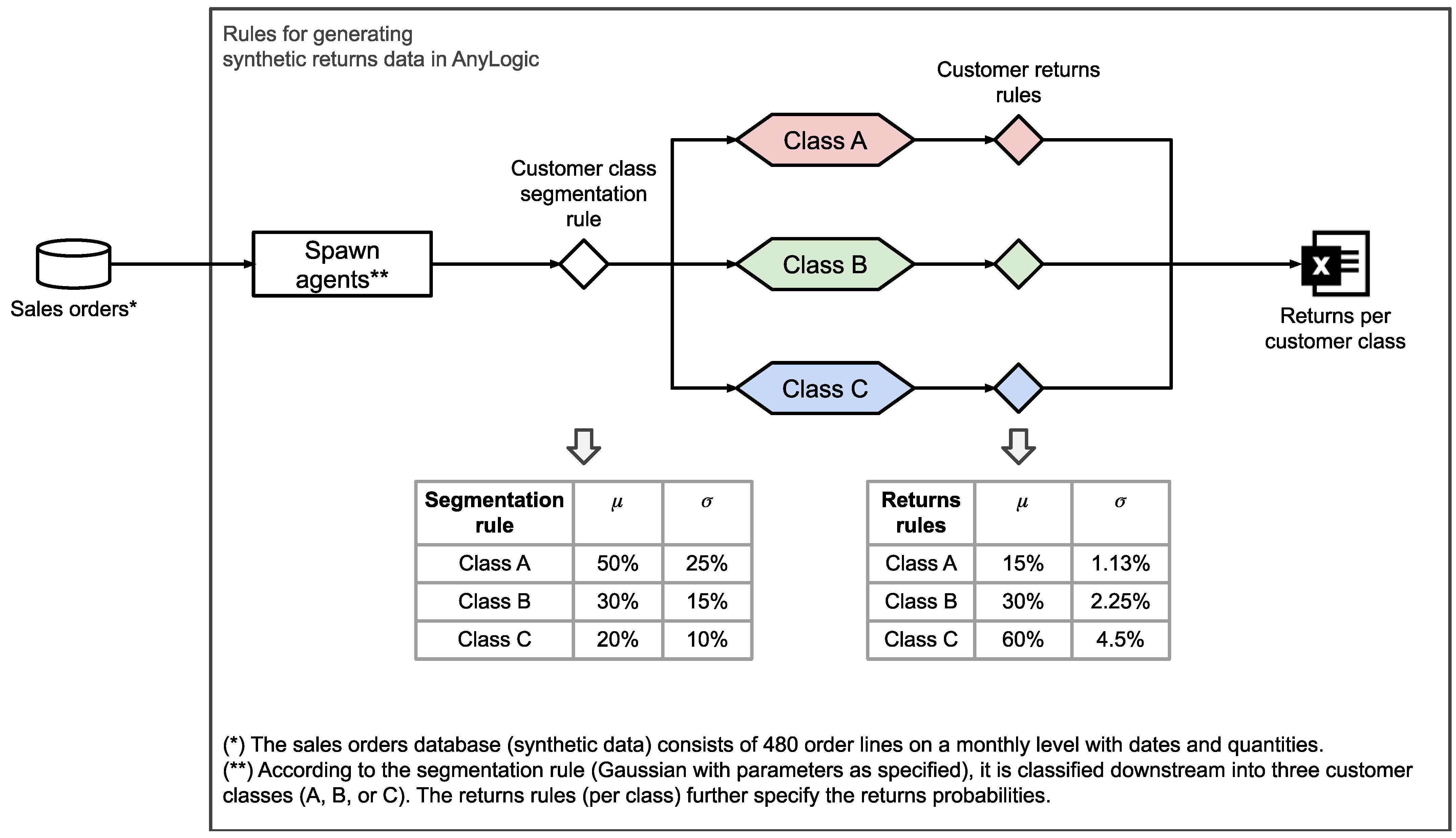
The experiment involves a fictitious company, Acme, attempting to improve its product sales and returns-forecasting process. The company uses a simple first-order exponential smoothing process—a simple but surprisingly hard-to-beat procedure [66]—and would like to evaluate the benefits of implementing an advanced machine learning algorithm, especially for returns. The basic assumption that returns forecasting can benefit from an algorithm more sophisticated than Acme’s current univariate (or single-variable) forecasting method is well founded. Specifically, more sophistication afforded by a multivariate approach might improve forecasting accuracy by using additional (leading) indicators, such as historical sales in the case of forecasting returns.
Although a simple comparison of forecast accuracy between the two approaches is a reasonable starting point for evaluating the potential benefits, it is often insufficient. The insufficiency stems from the forecasting process being just one among several processes in end-to-end process chains that encompass forward (material flow from suppliers towards customers) and returns flows (where the customer becomes the supplier for the post-consumer product [67]). Therefore, it is critical to check the local intervention (the forecasting process in the case of this experiment) for unintended global consequences. At Acme, besides the planned machine learning model for forecasting, most other decisions are assumed to be based on rules of thumb or heuristics. Therefore, a systemic assessment (checking if the locally rational algorithmic component translates globally, given that there is a mix of algorithmic and human rationality at this level) of the comingling of human and algorithmic decisions entails modeling the relevant parts of the adjacent production and order-fulfillment processes.

4.2. Data

The experiment (see Figure 1 for experimental protocol) uses a seasonal time series from the M forecasting competition [68] to generate a synthetic sales dataset by first decomposing it (into trend-cycle, seasonal, and remainder components) and subsequently constructing samples with similar demand characteristics.
Regarding the returns time series, the assumption is that Acme has three classes of customers with distinct returns characteristics or profiles (where a profile is a specific combination of the mean and standard deviation of returns that follows a normal distribution). A discrete event-simulation model built in AnyLogic [69] on this assumption generates the requisite returns data. It first spawns customer “agents” (based on the sales data) and sorts them randomly into three groups, assigning them their corresponding returns profiles. After a specified time offset, the model simulates an agent generating a product return per its profile—that is, a sample value, which stands for the number of units returned, is drawn from a normal distribution with the profile’s mean and standard deviation (see Figure 2).
The synthetic data generation process outputs a file consisting of 480 months of monthly sales (broken down by customer group) and returns data. Before model generation, the data undergo a further important processing step designed to tackle the problem of poor generalization common in ML.
Poor generalization performance, or the phenomenon of overfitting, is when model performance deteriorates severely on unseen data. It typically happens when the model learns spurious correlations or memorizes inputs [70] to return good training performance that does not translate to good performance in the real world. The usual recommendation to avoid overfitting is to split the data into train, test, and validation sets [71], which the experiment adopts by splitting the data according to a 60/10/30 ratio. Although several specific techniques exist to perform the split, the experiment takes a simple holdout validation approach. In this variant, the training set determines model parameters, the validation set helps fine-tune those parameters, and the test set forms the basis for the final performance evaluation. Given the relatively simple nature of the original seasonal sales data with a limited number of possible features and the synthetic data generation approach (affording finer control over the noise, thus placing modest demands on sample size), there are no grounds for more complex treatments such as K-fold and iterated K-fold validation more suited to feature-rich/data-sparse contexts [70].

4.3. Main Components

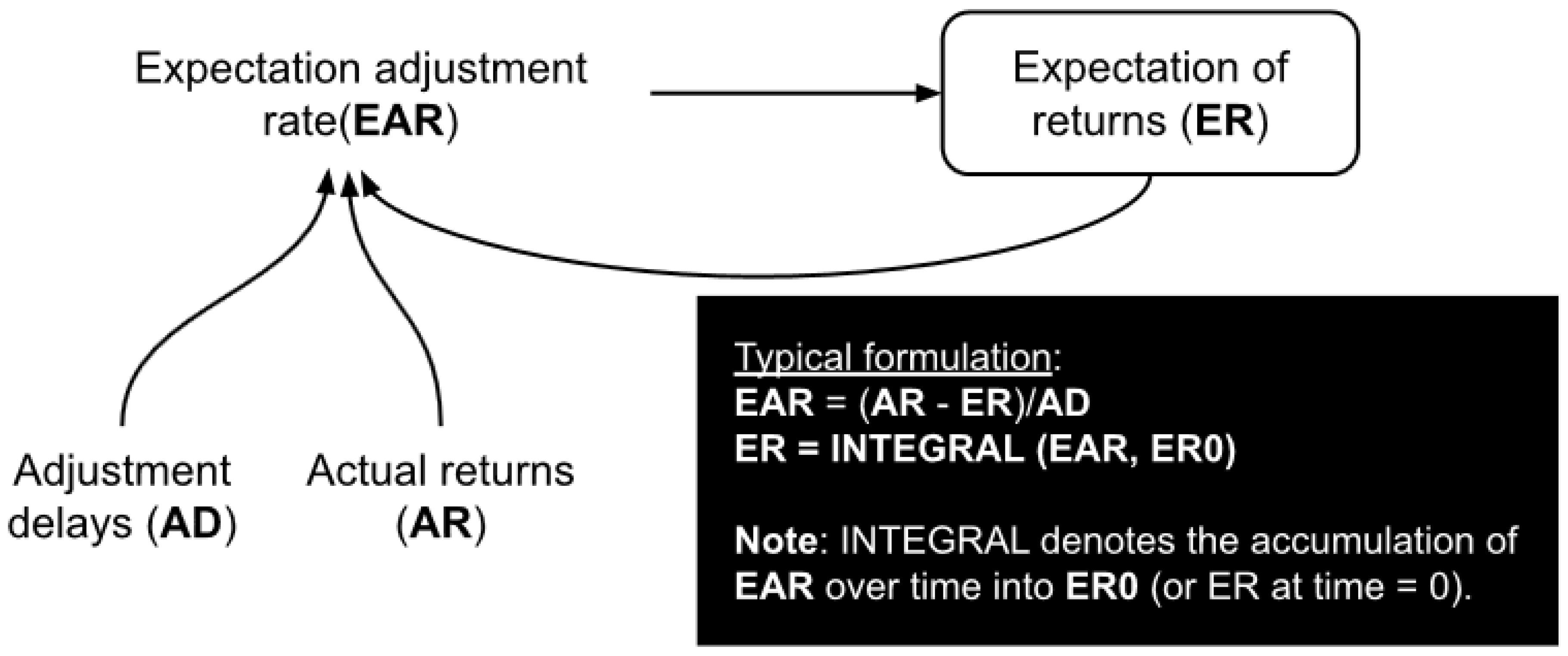
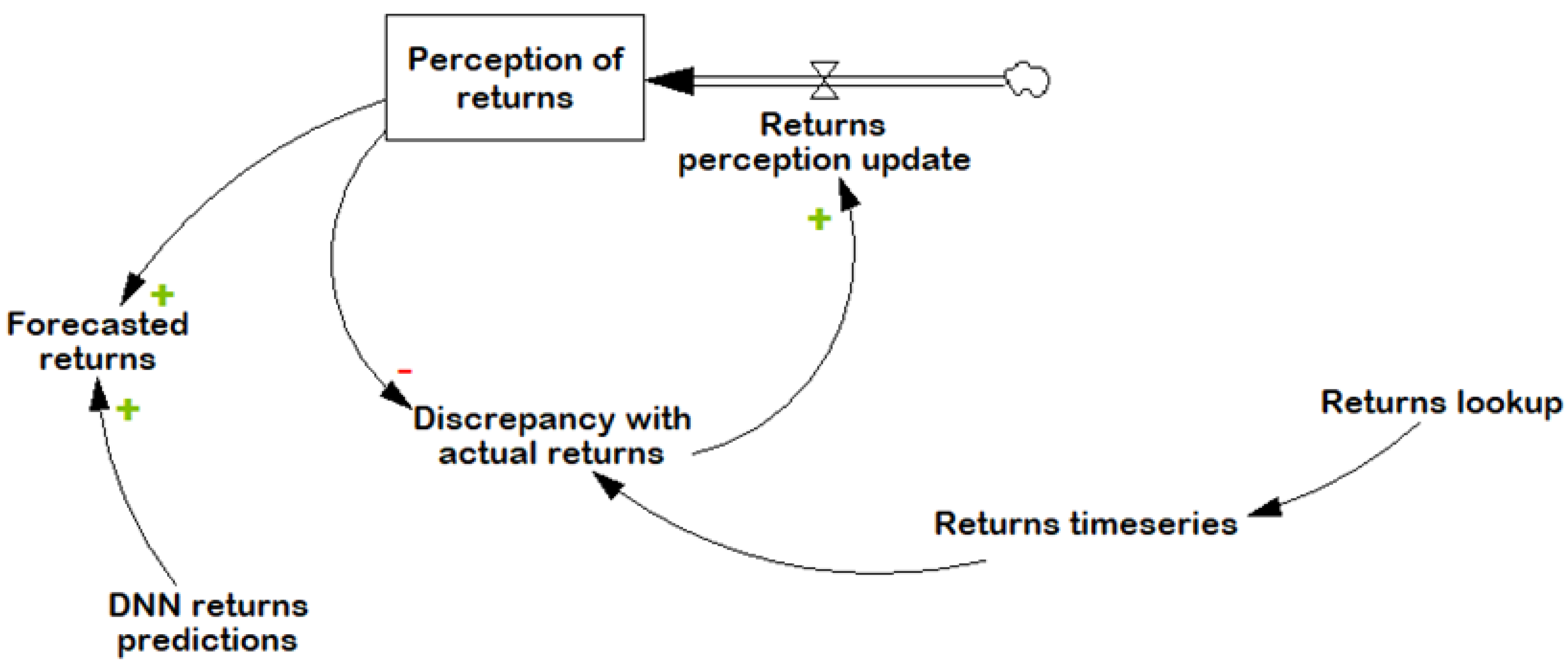
4.3.1. Modeling Judgmental Forecast

System dynamics offers various techniques for modeling simple rules that characterize human decisions in most contexts [57]. One such representation is the so-called anchor-and-adjust [72], which produces an effect similar to the first-order exponential smoothing procedure, which serves as the experiment’s current-state judgmental process for forecasting sales and returns. The term anchor-and-adjust alludes to a well-known fact from psychological research that humans, when tasked with estimation, “anchor” on an initial value and adjust it according to the cues they receive [73]. Despite the apparent simple-mindedness of the procedure, there is abundant empirical evidence [72] that supports its use by decision-makers in contexts where the sheer number of influencing factors make satisficing rational in intention.
In the experiment’s forecasting process, the initial value or anchor is a historical average of sales or returns. The value undergoes continuous adjustments upon receiving informational feedback (actual sales or returns orders). The adjustment rate, which depends on empirical details regarding such factors as feedback delays experienced by an organization, is set to three months in Acme’s case. A delay of three months roughly corresponds to setting the smoothing constant to 0.3 when using the exponential smoothing procedure. Although it is possible to search (for instance, using a grid search technique) for a more optimal value, it is not essential given that the experimental objective only relies on the claim that ML represents any improvement over a heuristic approach. In other words, the qualification criterion for local rationality is that ML is somewhat better than the extant approach. Furthermore, as we will also see, the magnitude of the difference in accuracy between the two approaches renders any fine-tuning effort of the delay parameter moot.

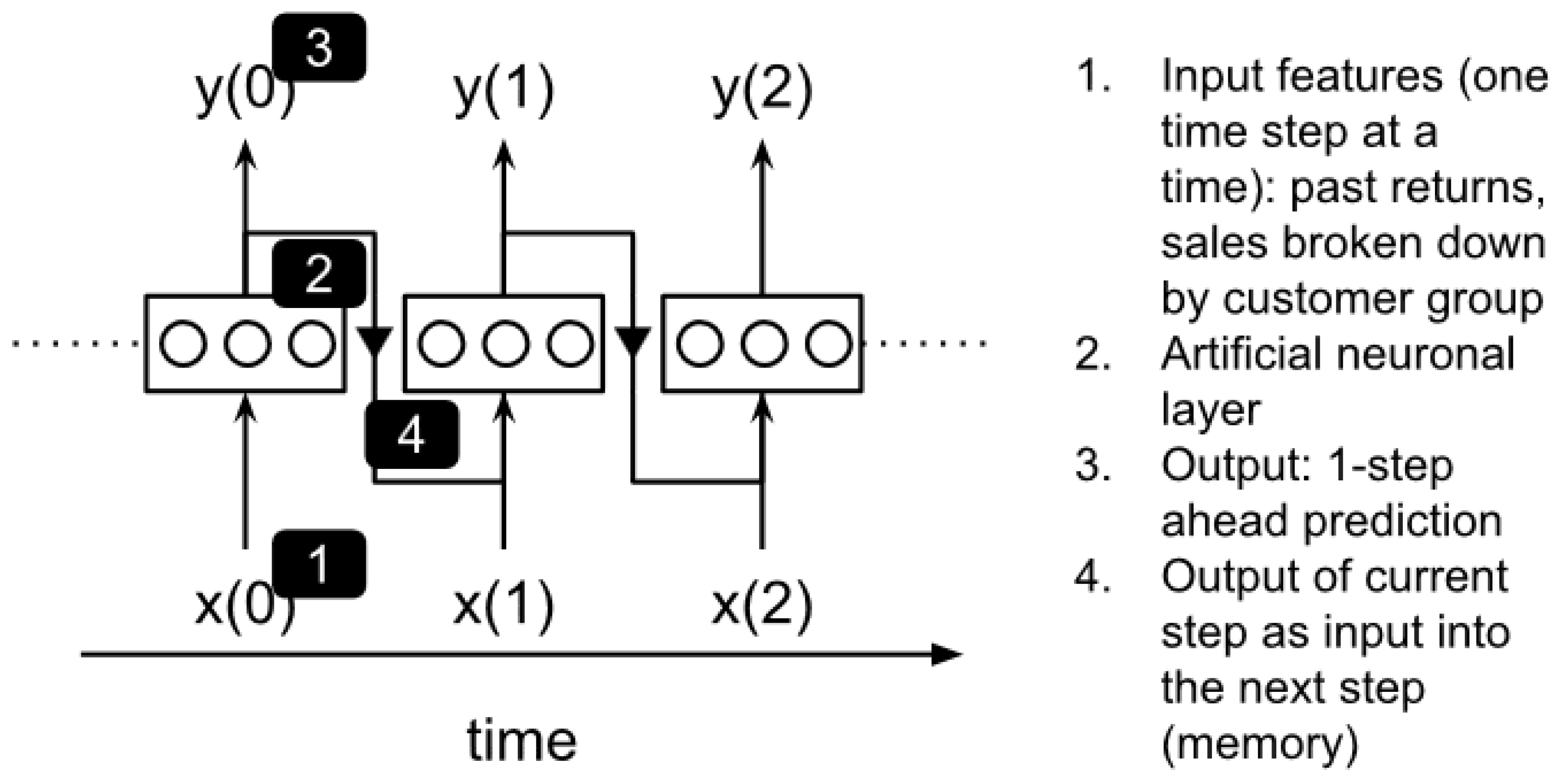
4.3.2. Modeling ML Forecast

As mentioned earlier, the primary focus of the ML method in Acme’s context is improving returns forecast accuracy. Since sales (split by the three customer groups) serve as an early indicator for future returns (except, potentially, historical returns), the intuition is apparent behind using an ML algorithm that can learn how the two relate without explicit instructions. More technically, an ML model can learn, from training samples (consisting of input/output pairs), the transformation from the input (set of early indicators) to the output (future returns) that minimizes prediction errors. This description corresponds to a supervised learning regime.
However, the requirements for sequential data (in this context, time series) are slightly more stringent—the architecture must be capable of maintaining temporal ordering. From this perspective, there are two basic ML architectures: feedforward networks that flatten the inputs, hence their lack of means to carry forward information meaningfully, and architectures with a feedback loop. A recurrent neural network (RNN) is an architecture that falls into the latter type, which the evaluation framework uses. An RNN can use its memory about earlier periods in a time-series setting and combine it with the current period while making a prediction. One can best imagine the process by “unrolling (the network) through time” [74]; that is, imagining the network processing each of the periods sequentially. In the simplest case of a network of a single artificial neuron, it receives as input both the current period value and the output of the previous period (usually initialized to zero at the start). Thus, at any given period, the additional input—the output of the previous period—is akin to the memory of the entire past, which influences predictions.
For the RNN implementation, the framework uses the Keras API, which offers convenient routines for training deep learning models [70]. In Keras, there are three types of RNN available: SimpleRNN, long short-term memory (LSTM), and the gated recurrent unit (GRU). Each type shares the basic idea of carrying over information when processing sequential information such as time series. The crucial difference between RNN and both LSTM and GRU lies in the latters’ relative ability to handle long sequences. Since the backpropagation procedure has to deal with a significantly deeper network, given the unrolling through time, SimpleRNN (the vanilla implementation) suffers from a debilitating memory loss problem. It is a problem that LSTM and GRU specifically address, partly by being more discerning about what to retain and what to forget [74]. In the experiment, the sales model uses LSTM given the long historical sales horizon (36 months since there are seasonal effects). For the returns scenario, the experiment uses GRU as it performed better during the parameter tuning phase.
Figure 3 and Figure 4 below provide a schematic representation of the ML (using RNN for illustrative purposes) and heuristic approaches.

4.4. Execution and Results

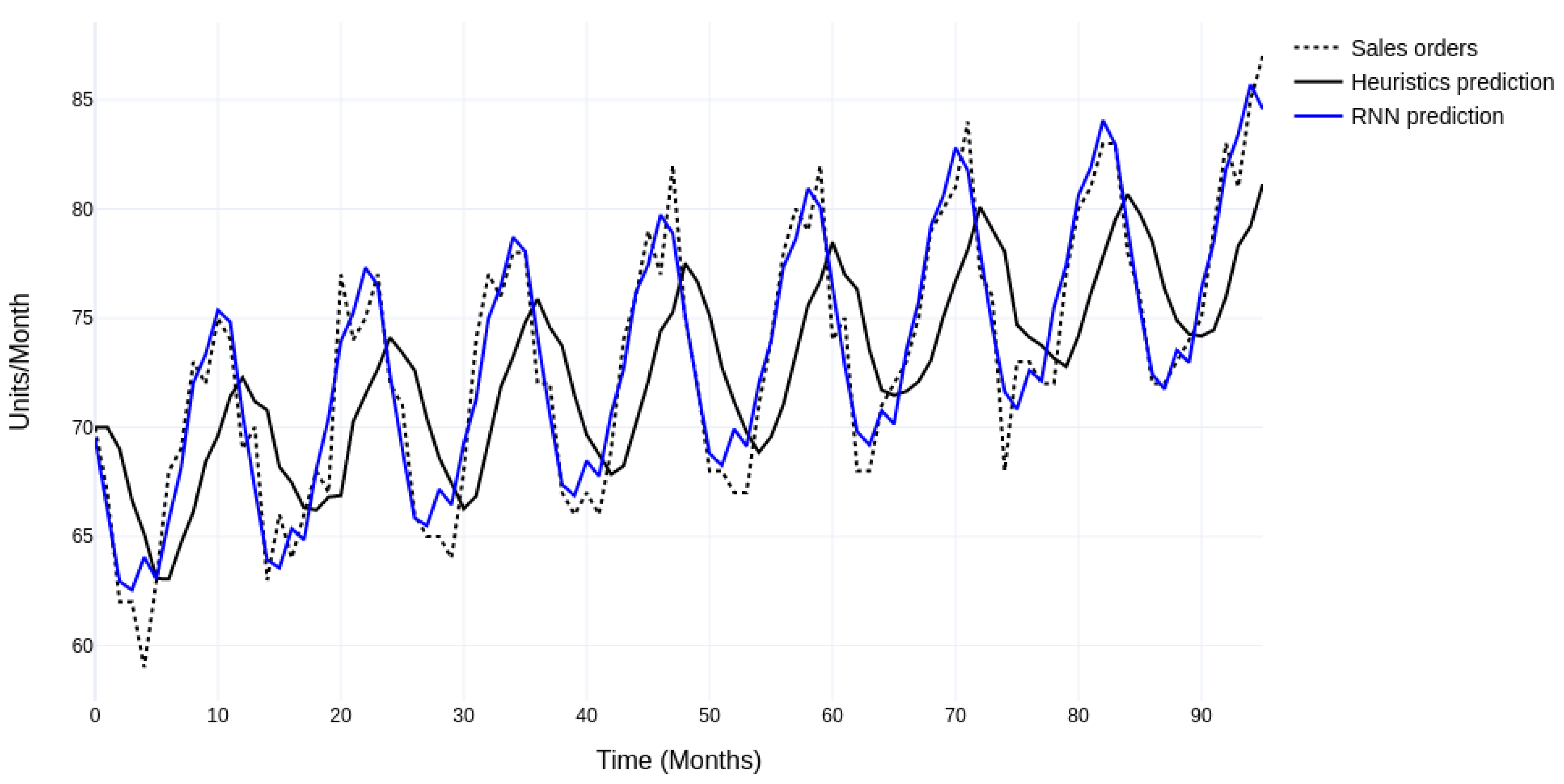
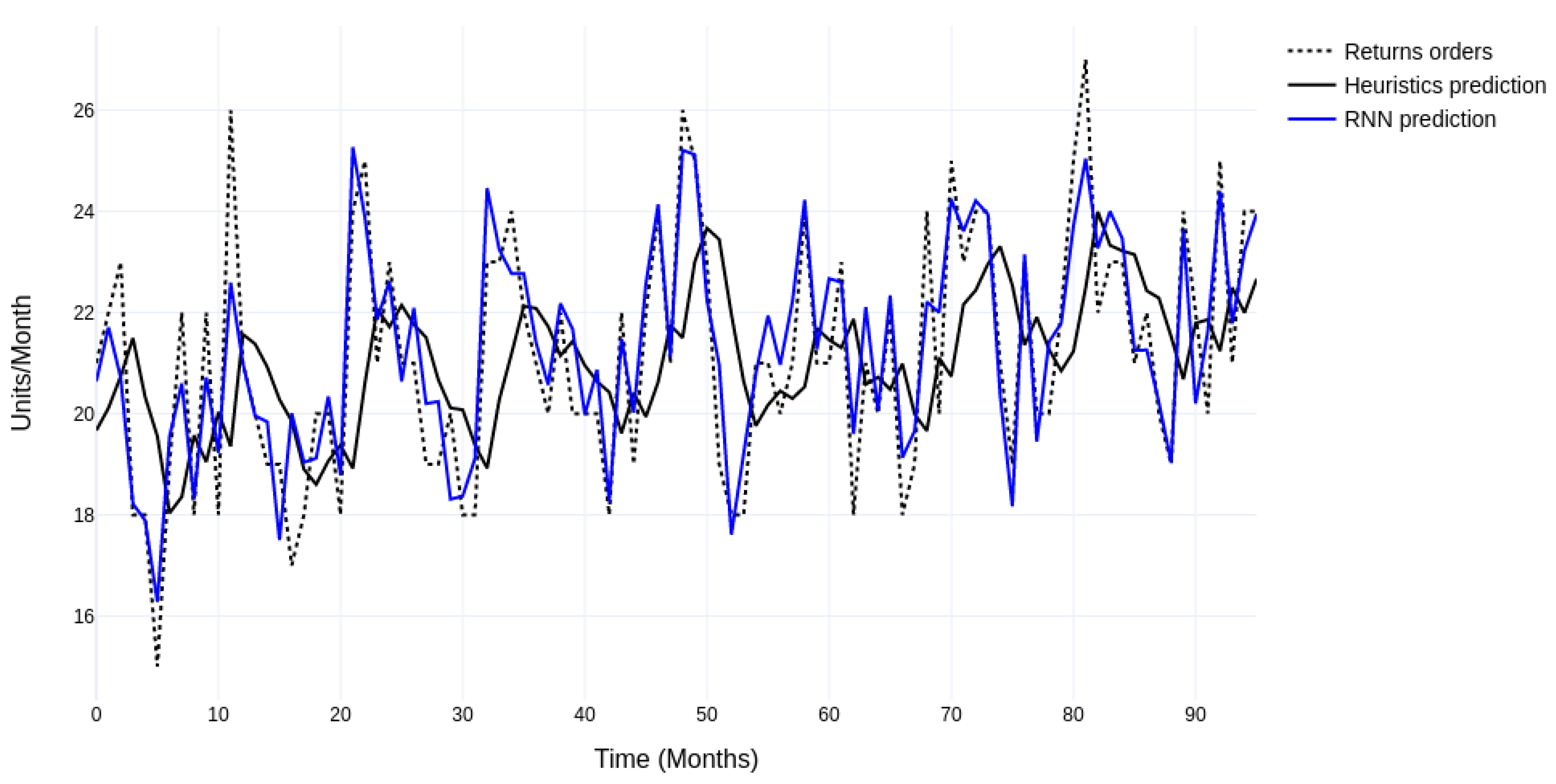
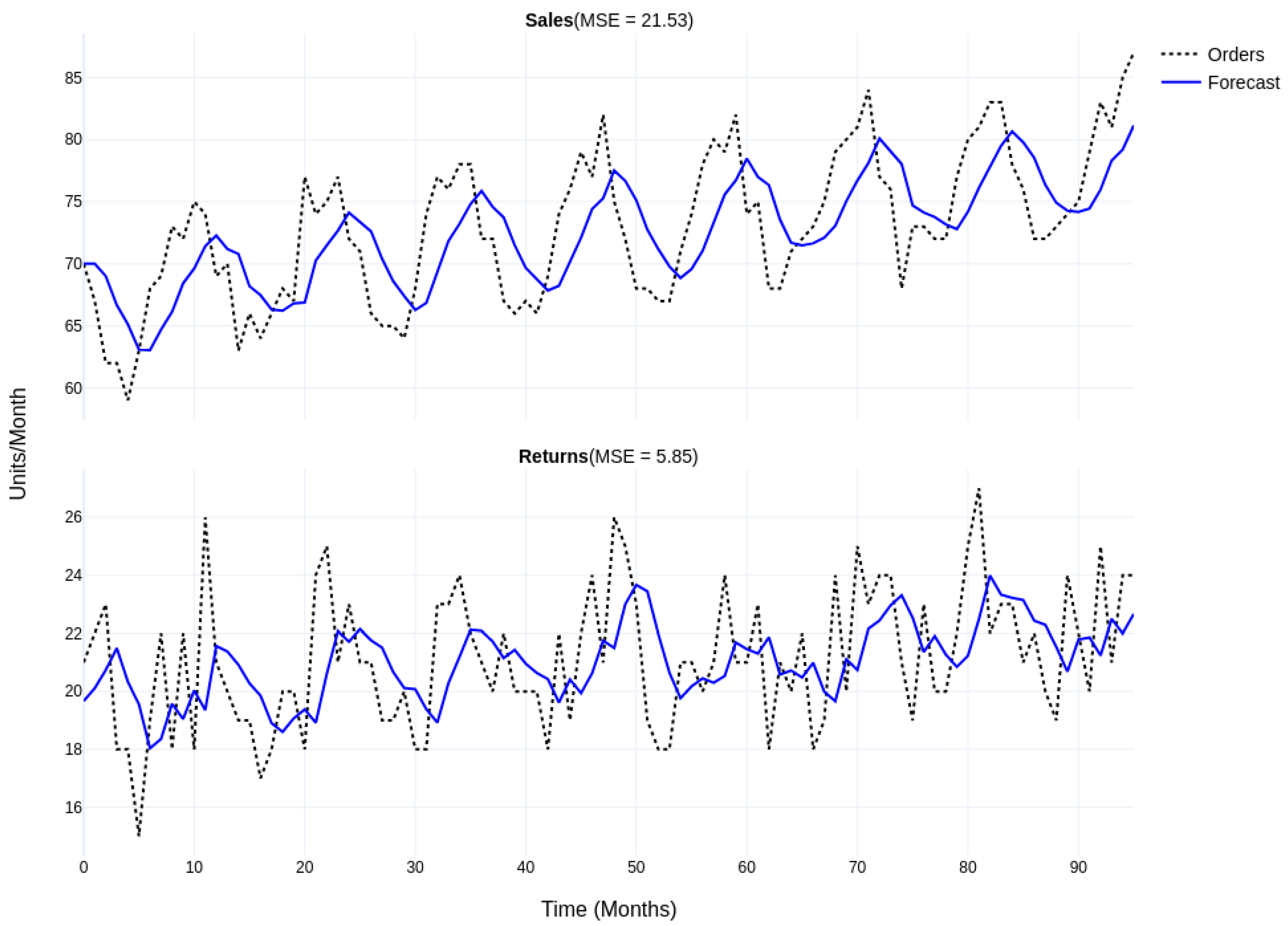
4.4.1. Comparing Stand-Alone Forecasting Performance

The first stage of the experiment is a straightforward comparison of the forecast accuracy of the RNN and heuristic approaches. The RNN sales- and returns-forecasting models have the following main parameters (see Table 1): a single hidden layer (the former with 225 units and the latter with 150 units), a dropout rate of 10%, a mean squared error (MSE) loss function, and 150 epochs of training. As noted earlier, the sales model uses LSTM and a returns model GRU. (Including dropouts is another effective means to avoid overfitting as the dropping out of units from the network with a certain probability (rate) leads to more robust overall learning since it trains the elements to be more self-reliant and discourages excessive reliance on specific inputs.)
After model fit, an evaluation of the model to assess overfitting (Figure 5) shows the converging training and validation loss curves, which indicates a robust fit. The canonical overfitting behavior is when training loss decreases while the validation loss increases—the divergence is predictive of poor generalizability.
Carrying out a partial model test to verify intended rationality [56] by embedding the forecasting routine in the system dynamics model shows that the accuracy (measured using the mean squared error metric) of RNN is 87.4% better for sales (21.4 compared to 2.7) and 81% better for returns (5.8 compared to 1.1). Figure 6 below shows the system dynamics model for returns; the sales model follows the same structure. Table A1 in Appendix A provides a complete list of the parameters for the system dynamics model.
The graphs below (Figure 7 and Figure 8) compare the RNN and heuristic predictions against the actual sales and returns orders. At first glance, a more significant improvement in sales-forecasting accuracy with RNN might be surprising. However, this is because the sales time series shows seasonality, but the anchor-and-adjust heuristic does not account for seasonal factors, providing a satisfactory explanation.
As an additional sanity check, a comparison of the accuracy of the heuristic to a simple exponential smoothing procedure using the Statsmodels library [75] (with a smoothing equivalent to a delay of three months, as described earlier) shows that the MSEs are roughly the same (Figure 9). It confirms the magnitude of the local improvement indicated earlier.

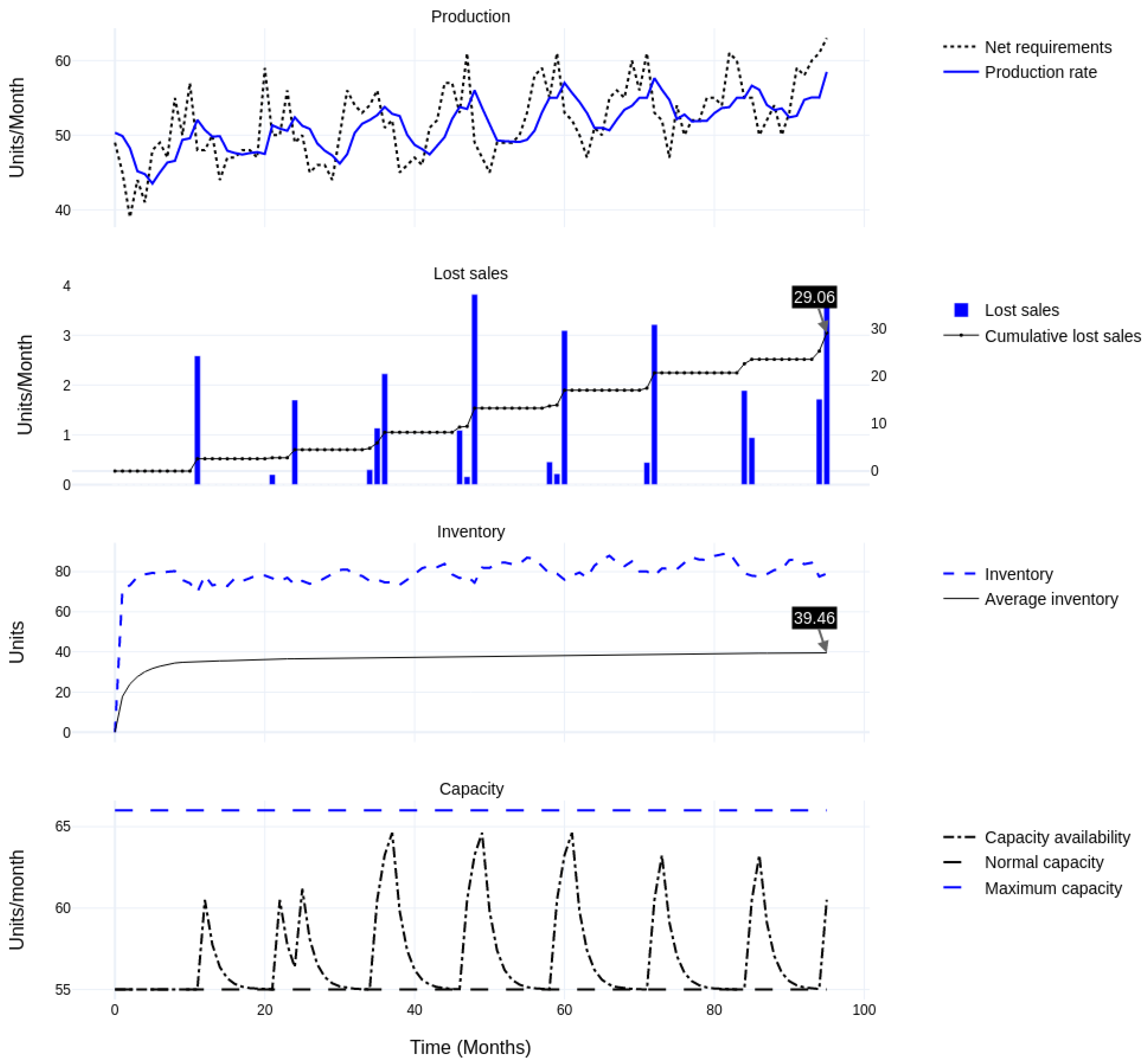
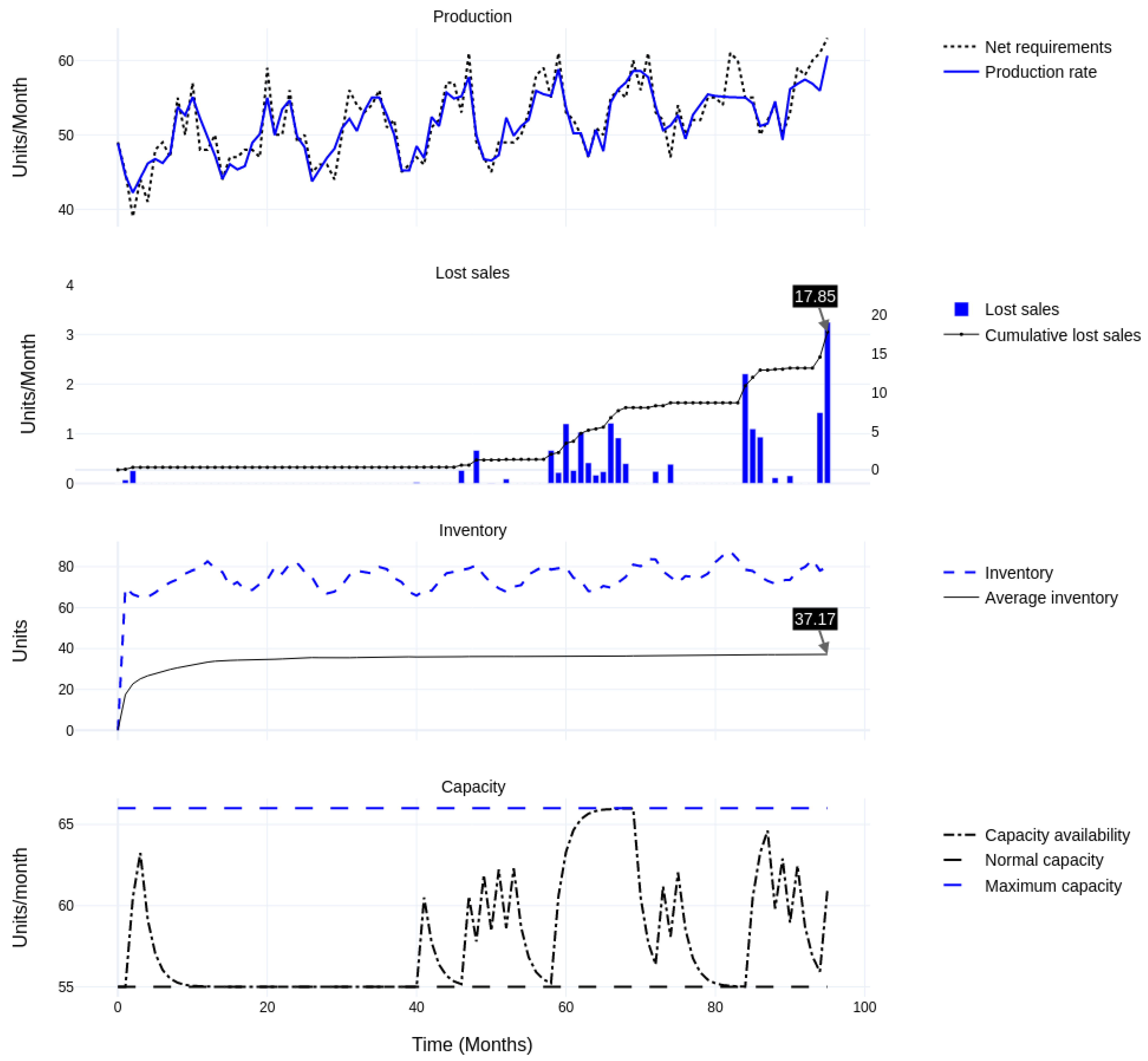
4.4.2. Comparing Overall System Performance
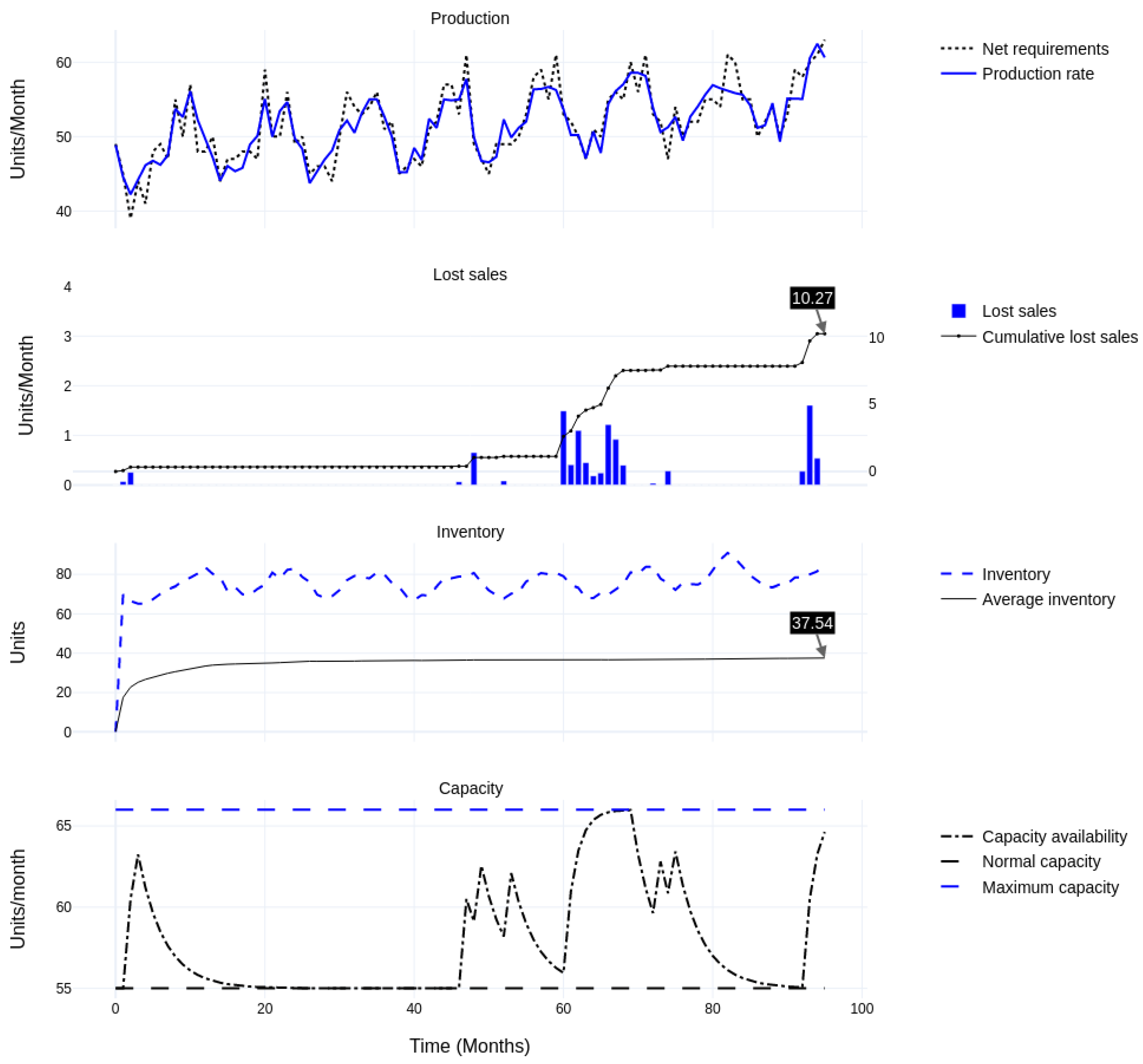
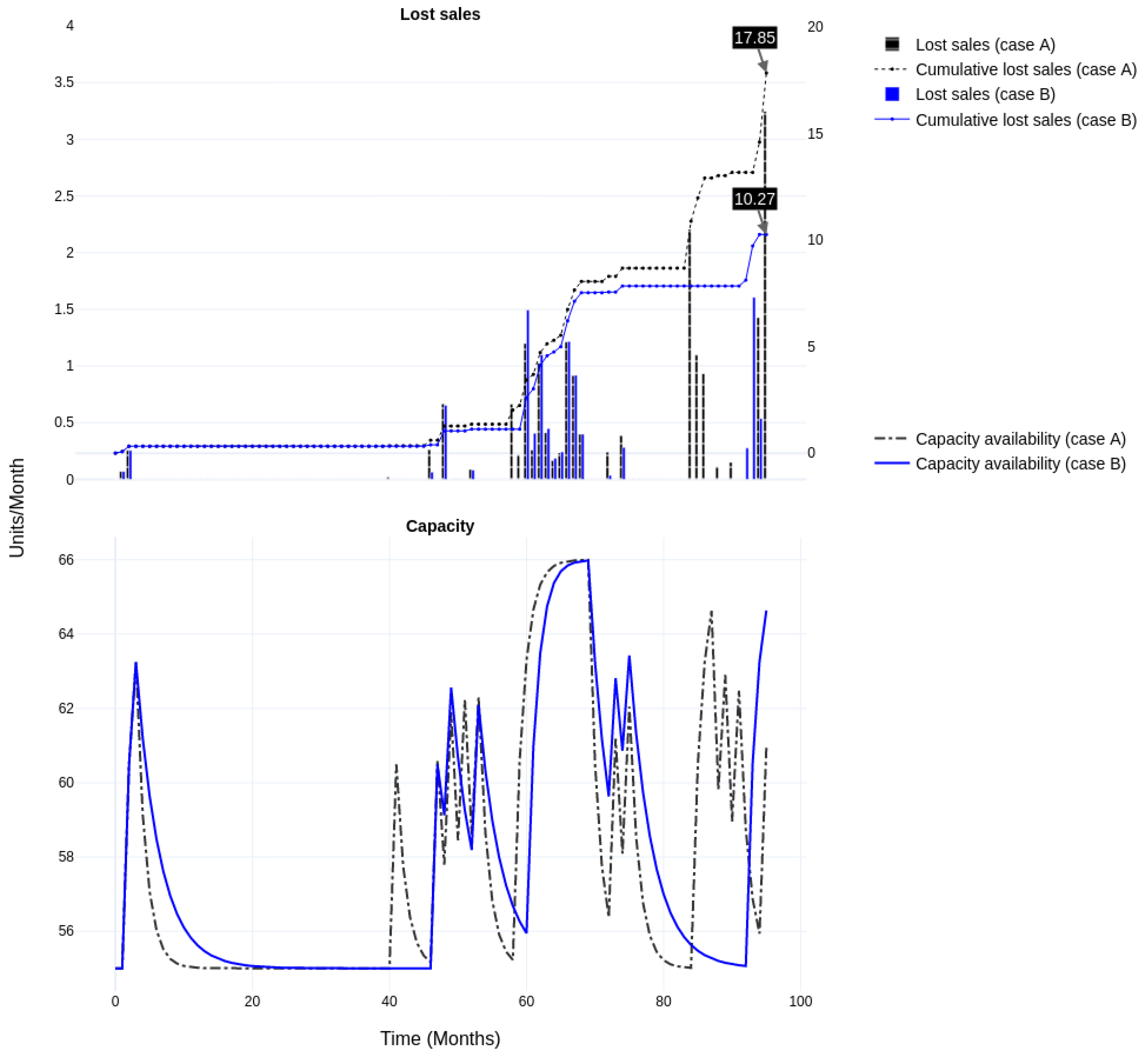
The second and most crucial stage involves evaluating the impact of the forecasting intervention (use of RNN) in its proper context by including relevant aspects of Acme’s overall forecasting, order fulfillment, and extended production processes. A decision parameter in the whole-model simulation (Figure 10a) determines the source of predictions (for sales and returns)—heuristics (or judgmental) or RNN. If set, PySD substitutes a hook in the model with a function that makes online predictions that integrate with the rest of the model (Figure 10b). Otherwise, judgmental or heuristic predictions take effect (Figure 10c). Acme follows a make-to-stock strategy, implying that it fulfills orders from inventory. Here (order fulfillment sector in the figure below), the system dynamics model includes simple rules to satisfy orders as they come in and to ascertain backorders and lost sales if there is a shortage—in other words, when the forecast is inaccurate. If the delivery lead time exceeds the goal, delivery pressure (a function of backlog) builds up, resulting in lost sales if the delay exceeds the tolerance limit (Figure 10d). Production orders are simply the difference between forecasted sales and returns in the production sector. For simplicity, the experiment assumes a negligible production lead time (a few days) relative to the planning periodicity (of months). At the end of the month, the forecasts generate production orders, assumed to be available as inventory at the start of the following period.
The decision rules discussed thus far are operational (in their evolutionary theory of economic change, Nelson and Winter use the term “operating characteristics” to characterize such rules [43]). However, there is a routine in the capacity management sector that is at a higher level, typically considered tactical by supply chains. It is a routine that calibrates the available capacity and is a crucial determinant of overall performance. The routine is responsible for augmenting capacity under delivery pressure (Figure 10e). Augmentation increases the capacity at a rate defined by the ramp-up delay (Figure 10f) to a maximum capacity determined by the available discretionary capacity. On the other hand, capacity normalization happens as the pressure eases. The equation for delivery lead time overshoot captures the easing of delivery pressure. This is the difference between the goal delivery lead time and the delivery lead time outlook (the ratio between the backlog and the current clearance rate). As the overshoot moves close to zero—all other things being equal—the normalization rule down-regulates the available capacity until it reaches the standard available capacity.
As all the rules in the whole-model simulation, except the source of predictions, are the same, verifying the effect of improved forecast accuracy on the overall performance is allowed. In an ideal scenario—perfect forecast accuracy—the lost sales are zero, and the average inventory equals half of the average production orders (since the planned production is available at the start of the period and the consumption of inventory by sales is assumed to proceed at a constant rate). Thus, lost sales and average inventory are the outcome metrics—closer to actual business performance—that provide a window into how well the process metric (forecast accuracy) translates to improved performance, seen holistically.

Base Case

As the first step of the whole-model simulation, setting the capacity profile to two months each for ramp-down and ramp-up and a 20% discretionary capacity, the results show a 39% improvement in lost sales (RNN over heuristics) performance and a 6% improvement in inventory (see Figure 11 and Figure 12, and Table 2).
At first glance, the results seem to live up to the promise of the forecast accuracy gains of RNN over heuristics. However, studying the graphs gives pause as it suggests that there are further improvements to be made. Focusing on the lost sales and capacity subplots and comparing the RNN and heuristics graphs, one sees that the capacity profile in the case of RNN has significantly more spikes. The lost sales in the case of RNN are also much more densely clustered compared to heuristics. This behavior results from RNN’s superior ability to capture the peaks and troughs in customer demands (one can see this by comparing the production rate curves). In particular, the inability of heuristics to anticipate the troughs results in excess inventory. The inventory build-up obviates the need for sustained additional capacity in the case of heuristics—thus, the capacity availability curve is smoother.
On the other hand, the much-improved forecast accuracy of RNN translates to the production rate closely chasing actual demands, thereby leading to a leaner inventory profile. An additional consequence of the better anticipation of lows is that capacity seems to normalize too quickly during periods with “rugged” peaks. This suggests a simple adjustment (an increase) to the capacity ramp-down delay. Intuitively, a slower ramp-down should allow the provisioning of some buffer capacity to clear the backlog, even as the production rate continues to roughly trace the sharp turns in the demands.

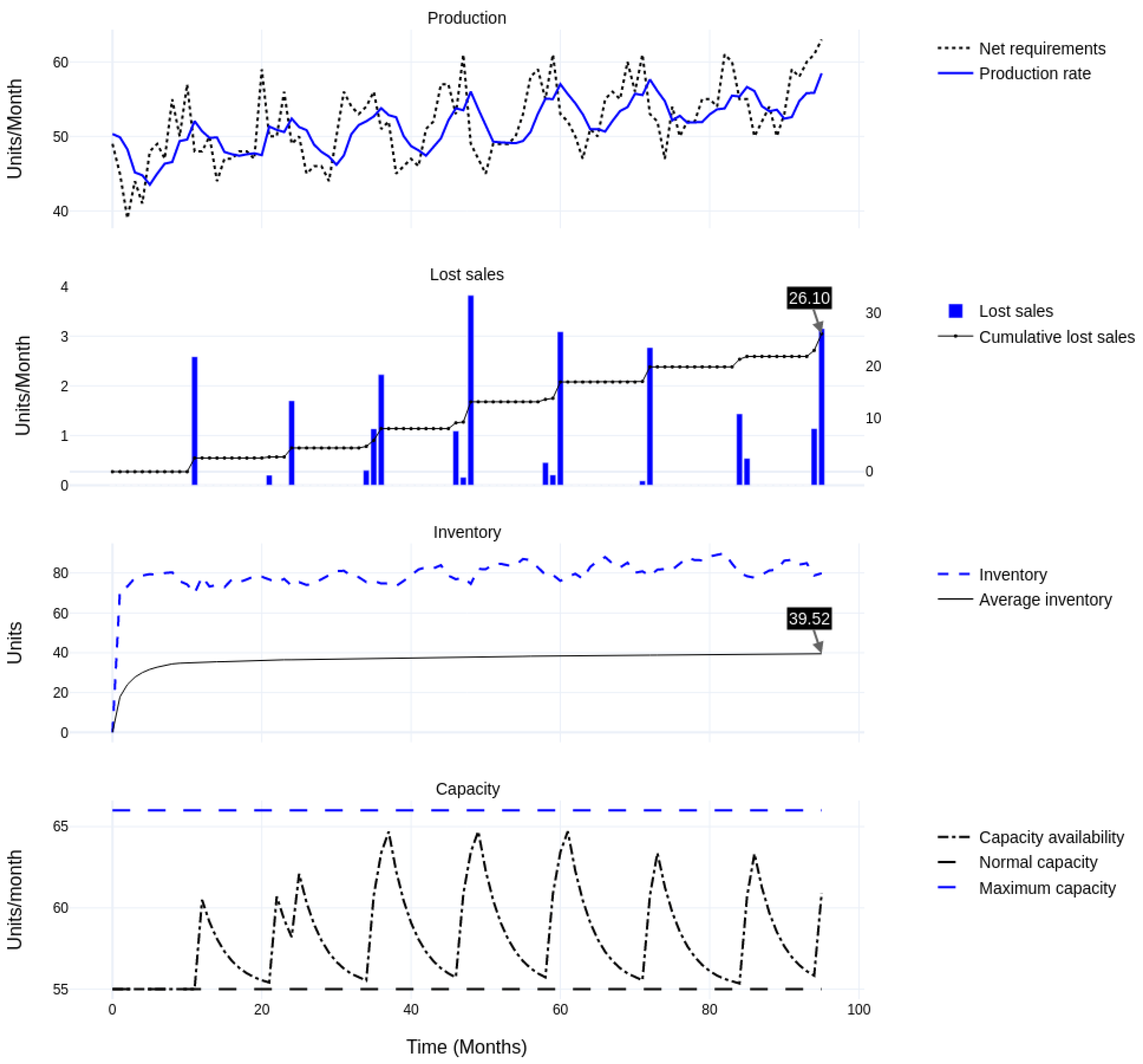
Heuristic Adjustment

After adjusting the ramp-down to four months (up from two months), the results show a 61% improvement in lost sales (RNN over heuristics) performance and a 5% improvement in inventory. This represents a 42.5% improvement in lost sales (with a slight 1% degradation in inventory performance) for RNN over the base case (see Figure 13 and Figure 14, and Table 2).
As intuitively hypothesized, the improvement in the case of heuristics over the previous scenario is minor in comparison (10% improvement in lost sales and a 0.2% degradation in inventory performance) to RNN, given its tendency to build excess inventory. Furthermore, as the capacity utilization for RNN is only slightly more than heuristics (3% more; 57.8 units/month versus 56.1 units/month), the nearly cost-neutral rule adjustment projects substantial overall gains.
A graph that overlays lost sales and the capacity profiles in the second scenario for RNN (see Figure 15) confirms our intuition regarding why RNN benefits disproportionately from this rule change. The capacity availability profile in the second case has fewer spikes owing to the more gradual ramp-down, which allows for additional buffer capacity (relative to case A) for clearing the backlog, resulting in less dense clustering of lost sales than before.

5. Discussion and Conclusions

Despite the rapid pace of progress in ML, there are concerns about the disconnect between innovation and adoption [9] and between investments and value (e.g., [76,77]). A growing body of work reflecting on the state of ML notes the overemphasis of technology over transformation (e.g., [78,79]) and worker substitution over augmentation [15]. Consequently, there is neglect in studying the unique ways by which humans and ML can jointly unlock significantly more value (e.g., [14,22,80]). We contribute to the conversation by adopting the view that ML is a technological asset that combines in an organizational-specific manner with other assets, chiefly personnel, to generate value. In the following paragraphs, we discuss the primary insights from the simulations performed using our proposed quantitative model that is suitably subjective (and holistic) in its conceptualization of the value-generation process. We also note the implications of these insights and how they relate to other works of a more conceptual/abstract nature in this area.
Our simulations have highlighted that, although procedurally rational, local process improvements (measured via process metrics) do not automatically translate to commensurate overall benefits (measured via outcome metrics). The system dynamics approach provides an elegant way to confirm the rationale of the improvement (in this case, the ML intervention) through partial model tests before proceeding to whole-model simulations to check for unintended global consequences. Although, as noted earlier, the idea of partial-model tests is not new [56], employing the idea when the improvement comes from ML is novel. It assumes greater significance in light of recent work [17] on organizational learning (using an abstract agent-based modeling approach) in a human–ML collaborative context that shows that ML strongly influences the classic explore–exploit trade-off [81]. Specifically, since ML agents do not subscribe to preexisting organizational mental models, they tend to facilitate nimbler exploration of the performance landscape. However, this also amplifies the type of risk our experiments illustrate (entering an organization into operating regimes with an increased likelihood of untested decision routines or operating characteristics that might produce dysfunctional global outcomes). The new dynamics caused by the introduction of ML forecasting in our experiment underscores this point.
Before ML, the incumbent heuristic method was slow to react to peaks and troughs in actual sales and returns (because of the inertia inherent in the anchor-and-adjust heuristic, current perceptions change only slowly). More pertinent to the earlier point regarding exploration, ML predictions (from the forecasting process) that are closer to actual values readily expose the inadequacy of the adjacent capacity management process. For instance, some high values that ML predicts are more than the standard available capacity, and the rules for using additional discretionary capacity suffer from latency, leading to poor order fulfillment performance. The example confirms the folk wisdom in manufacturing, supported by rigorous research, that saving time at a non-bottleneck resource is a mirage [82]. Translated to the experiment, the forecast improvement beyond a point collides with the capacity bottleneck, which limits the performance (unless addressed). This example reinforces the point about broadening the scope of analysis—organizational decision-making involves complex feedback loops that make it unrealistic to anticipate high-level outcomes accurately.
In addition, the approach taken in the experiment to alleviate the problem demonstrates the importance of complementarity between decision pairs. Concretely, the improvement took the form of reducing the delay in using the discretionary capacity. In general, ML increases the “clock speed” [83] of an organization, and the decision structures must keep pace, for example, through decentralization that tends to reduce the number of levels a decision has to pass through (reducing delays).
A further implication of bottlenecks preventing subsystem improvements cascading to the system level—discovered through a synthetic rather than an analytical view of performance—is how it provides a valuable frame for questions about the value of data. In case additional data (costly to acquire and process) push the system to an operating point that surfaces limiting constraints fixed in the short term (e.g., physical assets or lead times), it puts a cap on benefits. This, in turn, helps ascertain the value of data collection efforts. From a more technical standpoint, a systems lens strengthens the argument for a reasonable statistical baseline before attempting ML methods that usually require many predictors and complex nonlinear relationships (between predictors and the target variable) for their superior performance [84].
Treating data as instrumental to value (and not valuable in themselves) is a position that follows naturally from the causal modeling approach that is the bedrock of system dynamics simulation. Thus, the importance given to the data-generating process aligns with the position of the causal inference research community (gaining wider acceptance) that espouses the need for good explanations. In Pearl’s words, “empiricism should be balanced with the principles of model-based science” [62]. One can surmise the upshot of this from our simulations. By situating the forecasting process in the context of the end-to-end order-to-delivery process chain, the model makes prioritizing aspects of the explanation possible. For instance, one can focus on predictions that most impinge outcomes and pose “why” questions (see Figure 16) to understand if they are representative or a product of anomalous inputs. In this way, the proposed modeling approach contributes to the explanatory AI work by identifying what the “completeness” criterion (for evaluating explanations) must entail.

Author Contributions

Conceptualization, G.S. (Ganesh Sankaran); Methodology, G.S. (Ganesh Sankaran); Software, G.S. (Ganesh Sankaran); Validation, G.S. (Ganesh Sankaran) and M.A.P.; Formal analysis, G.S. (Ganesh Sankaran); Investigation, G.S. (Ganesh Sankaran); Data curation, G.S. (Ganesh Sankaran); Writing—original draft, G.S. (Ganesh Sankaran); Writing—review & editing, G.S. (Ganesh Sankaran), M.A.P. and G.S. (Guido Siestrup); Visualization, G.S. (Ganesh Sankaran); Supervision, M.A.P., M.K. and G.S. (Guido Siestrup); Project administration, M.A.P.; Funding acquisition, G.S. (Guido Siestrup). All authors have read and agreed to the published version of the manuscript.

Funding

This research received no external funding.

Institutional Review Board Statement

Not applicable.

Informed Consent Statement

Not applicable.

Data Availability Statement

The ML code, system dynamics simulation files, and data are available on GitHub under: https://anonymous.4open.science/r/aicollab-model-C108.

Conflicts of Interest

The authors declare no conflict of interest.

Credits

The “Excel” icon on pages 8 and 9 is by Gleb Khorunzhiy, the “Mind” icon on page 8 is by Med Marki, the “Decision” icon on page 8 is by Template, and the “Simulation Computer” icon on page 8 is by Ian Rahmadi Kurniawan; they were all sourced from thenounproject.com.

Appendix A

Table A1. System dynamics parameters.
VariableEquation or ValueUnits
Adjusted production rateIF THEN ELSE (“Use DNN?” = 1, MIN (Capacity, DNN predictions), MIN (Capacity, Judgmental production rate))Pcs/Month
BacklogINTEG (Sales orders − Fulfillment rate − Lost sales, 0)Pcs
CapacityINTEG (Capacity augmentation rate − Capacity normalization rate, Normal capacity)Pcs/Month
Capacity augmentation rateIF THEN ELSE (Delivery lead time overshoot > 0, Capacity flexibility/Capacity ramp-up time, 0)Pcs/(Month × Month)
Capacity flexibilityMaximum capacity − CapacityPcs/Month
Capacity normalization rateIF THEN ELSE (Delivery lead time overshoot > 0, 0, Excess capacity/Capacity ramp-down time)Pcs/(Month × Month)
Capacity ramp-down time2 (base case); 4 (heuristic adjustment)Month
Capacity ramp-up time2Month
Delay tolerance2Month
Delivery lead time goal1Month
Delivery lead time outlookIF THEN ELSE (Backlog = 0, 1, Backlog/Fulfillment rate)Month
Delivery lead time overshootMAX(0, Delivery lead time outlook − Delivery lead time goal)Month
Discrepancy with actual returnsReturns time series (Time/One month) − Perception of returnsPcs/Month
Discrepancy with actual salesOrder time series (Time/One month) − Perception of salesPcs/Month
Discretionary capacity0.2Dmnl
DNN predictionsDNN sales predictions (Time/One month) − DNN returns predictions (Time/One month)Pcs/Month
DNN returns predictionsThe result of RNN returns forecast is programmatically fed.Pcs/Month
DNN sales predictionsThe result of RNN sales forecast is programmatically fed.Pcs/Month
Excess capacityMAX(0, Capacity − Normal capacity)Pcs/Month
FINAL TIME96Month
Fulfillment rateMIN(Backlog, Inventory)/One monthPcs/Month
INITIAL TIME1Month
InventoryINTEG (Production rate + Return orders − Shipment rate, 0)Pcs
Judgmental production ratePerception of sales − Perception of returnsPcs/Month
Lost sales(Delivery lead time overshoot × Fulfillment rate)/Delay tolerancePcs/Month
Maximum capacityNormal capacity × (1 + Discretionary capacity)Pcs/Month
Net requirementsSales orders − Return ordersPcs/Month
Normal capacity55Pcs/Month
One month1Month
Order time seriesTest dataset for actual customer orders.Pcs/Month
Perception of returnsINTEG (Returns perception update, 19.67)
(Note: 19.67 is the initial value; equals the average of last 6 months of returns)
Pcs/Month
Perception of salesINTEG (Sales perception update, 70)
(Note: 70 is the initial value; equals the average of last 6 months of sales)
Pcs/Month
Production rateAdjusted production ratePcs/Month
Return ordersReturns time series (Time/One month)Pcs/Month
Returns perception updateDiscrepancy with actual returns/Update delayPcs/(Month × Month)
Returns time seriesTest dataset for actual customer returns.Pcs/Month
Sales ordersOrder time series (Time/One month)Pcs/Month
Sales perception updateDiscrepancy with actual sales/Update delayPcs/(Month × Month)
Shipment rateFulfillment ratePcs/Month
Update delay3Month
“Use DNN?”Programmatically set to switch between heuristic forecasting and RNN.Dmnl

References

  1. Brynjolfsson, E.; Mitchell, T. What can Machine Learning Do? Workforce Implications. Science 2017, 358, 1530–1534. [Google Scholar] [CrossRef]
  2. Dwivedi, Y.K.; Hughes, L.; Ismagilova, E.; Aarts, G.; Coombs, C.; Crick, T.; Duan, Y.; Dwivedi, R.; Edwards, J.; Eirug, A.; et al. Artificial Intelligence (AI): Multidisciplinary perspectives on emerging challenges, opportunities, and agenda for research, practice and policy. Int. J. Inf. Manag. 2021, 57, 101994. [Google Scholar] [CrossRef]
  3. Makridakis, S. The forthcoming Artificial Intelligence (AI) revolution: Its impact on society and firms. Futures 2017, 90, 46–60. [Google Scholar] [CrossRef]
  4. Mitchell, M. Why AI Is Harder Than We Think. arXiv 2021, arXiv:2104.12871. [Google Scholar]
  5. Chollet, F. On the Measure of Intelligence. arXiv 2019, arXiv:1911.01547. [Google Scholar]
  6. Marcus, G. The Next Decade in AI: Four Steps Towards Robust Artificial Intelligence. arXiv 2020, arXiv:2002.06177. [Google Scholar]
  7. Doshi-Velez, F.; Kim, B. Towards A Rigorous Science of Interpretable Machine Learning. arXiv 2017, arXiv:1702.08608. [Google Scholar]
  8. Blackman, R.; Ammanath, B. When—and Why—You Should Explain How Your AI Works. Harvard Business Review, 31 August 2022. Available online: https://hbr.org/2022/08/when-and-why-you-should-explain-how-your-ai-works(accessed on 28 October 2022).
  9. Zolas, N.; Kroff, Z.; Brynjolfsson, E.; McElheran, K.; Beede, D.N.; Buffington, C.; Goldschlag, N.; Foster, L.; Dinlersoz, E. Advanced Technologies Adoption and Use by U.S. Firms: Evidence from the Annual Business Survey; National Bureau of Economic Research: Cambridge, MA, USA, 2020. [Google Scholar] [CrossRef]
  10. Karp, R.; Peterson, A. Find the Right Pace for Your AI Rollout. Harvard Business Review, 25 August 2022. Available online: https://hbr.org/2022/08/find-the-right-pace-for-your-ai-rollout(accessed on 28 October 2022).
  11. Agrawal, A.; Gans, J.S.; Goldfarb, A. What to Expect from Artificial Intelligence. MIT Sloan Management Review, 7 February 2017. Available online: https://sloanreview-mit-edu.plymouth.idm.oclc.org/article/what-to-expect-from-artificial-intelligence/(accessed on 14 September 2021).
  12. Raisch, S.; Krakowski, S. Artificial Intelligence and Management: The Automation–Augmentation Paradox. Acad. Manag. Rev. 2021, 46, 192–210. [Google Scholar] [CrossRef]
  13. Shestakofsky, B. Working Algorithms: Software Automation and the Future of Work. Work. Occup. 2017, 44, 376–423. [Google Scholar] [CrossRef]
  14. Brynjolfsson, E.; McAfee, A. Will Humans Go the Way of Horses. Foreign Aff. 2015, 94, 8. [Google Scholar]
  15. Autor, D. Polanyi’s Paradox and the Shape of Employment Growth; NBER Working Papers 20485; National Bureau of Economic Research: Cambridge, MA, USA, 2014. [Google Scholar] [CrossRef]
  16. Melville, N.; Kraemer, K.; Gurbaxani, V. Review: Information Technology and Organizational Performance: An Integrative Model of IT Business Value. MIS Q. 2004, 28, 283–322. [Google Scholar] [CrossRef] [Green Version]
  17. Sturm, T.; Gerlach, J.P.; Pumplun, L.; Mesbah, N.; Peters, F.; Tauchert, C.; Nan, N.; Buxmann, P. Coordinating Human and Machine Learning for Effective Organizational Learning. MIS Q. 2021, 45, 1581–1602. [Google Scholar] [CrossRef]
  18. Malone, T.W. How Human-Computer ‘Superminds’ Are Redefining the Future of Work. MIT Sloan Management Review, 21 May 2018. Available online: https://sloanreview-mit-edu.plymouth.idm.oclc.org/article/how-human-computer-superminds-are-redefining-the-future-of-work/(accessed on 22 September 2021).
  19. Elena Revilla, M.J.S.; Simón, C. Designing AI Systems with Human-Machine Teams. MIT Sloan Management Review, 18 March 2020. Available online: https://sloanreview.mit.edu/article/designing-ai-systems-with-human-machine-teams/(accessed on 8 September 2021).
  20. Puranam, P. Human-AI collaborative decision-making as an organization design problem. J. Org. Design 2021, 10, 75–80. [Google Scholar] [CrossRef]
  21. Shrestha, Y.R.; Ben-Menahem, S.M.; von Krogh, G. Organizational Decision-Making Structures in the Age of Artificial Intelligence. Calif. Manag. Rev. 2019, 61, 66–83. [Google Scholar] [CrossRef]
  22. Brynjolfsson, E. The Turing Trap: The Promise & Peril of Human-Like Artificial Intelligence. Daedalus 2022, 151, 272–287. [Google Scholar] [CrossRef]
  23. Rahmandad, H.; Repenning, N.; Sterman, J. Effects of feedback delay on learning. Syst. Dyn. Rev. 2009, 25, 309–338. [Google Scholar] [CrossRef]
  24. Hogarth, R.M.; Lejarraga, T.; Soyer, E. The Two Settings of Kind and Wicked Learning Environments. Curr. Dir. Psychol. Sci. 2015, 24, 379–385. [Google Scholar] [CrossRef]
  25. Ethiraj, S.K.; Levinthal, D. Bounded Rationality and the Search for Organizational Architecture: An Evolutionary Perspective on the Design of Organizations and Their Evolvability. Adm. Sci. Q. 2004, 49, 404–437. [Google Scholar] [CrossRef]
  26. Knudsen, T.; Srikanth, K. Coordinated Exploration: Organizing Search by Multiple Specialists to Overcome Mutual Confusion and Joint Myopia. Adm. Sci. Q. 2013, 59, 409–441. [Google Scholar] [CrossRef]
  27. Simon, H.A.; Newell, A. Human problem solving: The state of the theory in 1970. Am. Psychol. 1971, 26, 145–159. [Google Scholar] [CrossRef]
  28. Glazer, R.; Steckel, J.H.; Winer, R.S. Locally Rational Decision Making: The Distracting Effect of Information on Managerial Performance. Manag. Sci. 1992, 38, 212–226. [Google Scholar] [CrossRef]
  29. Nonaka, I. The Knowledge-Creating Company. Harvard Business Review, 1 July 2007. Available online: https://hbr.org/2007/07/the-knowledge-creating-company(accessed on 6 September 2021).
  30. Narayanan, M.; Chen, E.; He, J.; Kim, B.; Gershman, S.; Doshi-Velez, F. How do Humans Understand Explanations from Machine Learning Systems? An Evaluation of the Human-Interpretability of Explanation. arXiv 2018, arXiv:1802.00682. [Google Scholar]
  31. Elgendy, N. Enhancing Collaborative Rationality between Humans and Machines through Data-Driven Decision Evaluation. In Proceedings of the 21st International Conference on Perspectives in Business Informatics Research (BIR), Rostock, Germany, 20–23 September 2022; p. 12. [Google Scholar]
  32. Sterman, J. System Dynamics: Systems Thinking and Modeling for a Complex World. Massachusetts Institute of Technology. Engineering Systems Division, Working Paper, May 2002. Available online: https://dspace.mit.edu/handle/1721.1/102741 (accessed on 2 June 2022).
  33. Gilpin, L.H.; Bau, D.; Yuan, B.Z.; Bajwa, A.; Specter, M.; Kagal, L. Explaining Explanations: An Overview of Interpretability of Machine Learning. In Proceedings of the 2018 IEEE 5th International Conference on Data Science and Advanced Analytics (DSAA), Turin, Italy, 1–3 October 2018; pp. 80–89. [Google Scholar] [CrossRef] [Green Version]
  34. Kasparov, G. Deep Thinking: Where Machine Intelligence Ends and Human Creativity Begins, 1st ed.; PublicAffairs: New York, NY, USA, 2017. [Google Scholar]
  35. Hassabis, D. Artificial Intelligence: Chess match of the century. Nature 2017, 544, 7651. [Google Scholar] [CrossRef]
  36. Simon, H.A. Administrative Behavior, 4th ed.; Free Press: New York, NY, USA, 1997. [Google Scholar]
  37. Lee, K.-F. AI Superpowers: China, Silicon Valley, and the New World Order, 1st ed.; Mariner Books: Boston, MA, USA, 2018. [Google Scholar]
  38. Reeves, M.; Ueda, D. Designing the Machines That Will Design Strategy. Harvard Business Review, 18 April 2016. Available online: https://hbr.org/2016/04/welcoming-the-chief-strategy-robot(accessed on 20 September 2021).
  39. Huang, M.-H.; Rust, R.; Maksimovic, V. The Feeling Economy: Managing in the Next Generation of Artificial Intelligence (AI). Calif. Manag. Rev. 2019, 61, 43–65. [Google Scholar] [CrossRef]
  40. Simon, H.A. The Sciences of the Artificial, 3rd ed.; The MIT Press: Cambridge, MA, USA, 1996. [Google Scholar]
  41. Klein, G.A. Sources of Power: 20th Anniversary Edition, 1st ed.; The MIT Press: Cambridge, MA, USA, 2017. [Google Scholar]
  42. Galbraith, J.R. Organization Design: An Information Processing View. INFORMS J. Appl. Anal. 1974, 4, 28–36. [Google Scholar] [CrossRef] [Green Version]
  43. Nelson, R.R.; Winter, S.G. Neoclassical vs. Evolutionary Theories of Economic Growth: Critique and Prospectus. Econ. J. 1974, 84, 886–905. [Google Scholar] [CrossRef]
  44. Gigerenzer, G.; Goldstein, D.G. Reasoning the fast and frugal way: Models of bounded rationality. Psychol. Rev. 1996, 103, 650–669. [Google Scholar] [CrossRef] [Green Version]
  45. Panchalavarapu, P.R.; De Kok, A.G.; Stephen, C.; Graves, C.S. (Eds.) 2004. Handbooks in Operations Research and Management Science: Supply Chain Management: Design, Coordination and Operation. Interfaces 2005, 35, 339–341. [Google Scholar]
  46. Devaraj, S.; Kohli, R. Performance Impacts of Information Technology: Is Actual Usage the Missing Link? Manag. Sci. 2003, 49, 273–289. [Google Scholar] [CrossRef] [Green Version]
  47. Wernerfelt, B. A resource-based view of the firm. Strateg. Manag. J. 1984, 5, 171–180. [Google Scholar] [CrossRef]
  48. Brynjolfsson, E.; Milgrom, P. 1. Complementarity in Organizations. In The Handbook of Organizational Economics; Princeton University Press: Princeton, NJ, USA, 2012; pp. 11–55. [Google Scholar] [CrossRef]
  49. Mithas, S.; Ramasubbu, N.; Sambamurthy, V. How Information Management Capability Influences Firm Performance. MIS Q. 2011, 35, 237–256. [Google Scholar] [CrossRef] [Green Version]
  50. Brynjolfsson, E.; Hitt, L. Computing Productivity: Firm-Level Evidence. Rev. Econ. Stat. 2003, 85, 793–808. [Google Scholar] [CrossRef] [Green Version]
  51. Haynes, C.; Palomino, M.A.; Stuart, L.; Viira, D.; Hannon, F.; Crossingham, G.; Tantam, K. Automatic Classification of National Health Service Feedback. Mathematics 2022, 10, 983. [Google Scholar] [CrossRef]
  52. Melville, N.; Gurbaxani, V.; Kraemer, K. The productivity impact of information technology across competitive regimes: The role of industry concentration and dynamism. Decis. Support Syst. 2007, 43, 229–242. [Google Scholar] [CrossRef]
  53. Will, J.; Bertrand, M.; Fransoo, J.C. Operations management research methodologies using quantitative modeling. Int. J. Oper. Prod. Manag. 2002, 22, 241–264. [Google Scholar] [CrossRef]
  54. Ackoff, R.L. The Future of Operational Research is Past. J. Oper. Res. Soc. 1979, 30, 93–104. [Google Scholar] [CrossRef]
  55. Frank, M.R.; Autor, D.; Bessen, J.E.; Brynjolfsson, E.; Cebrian, M.; Deming, D.J.; Feldman, M.; Groh, M.; Lobo, J.; Moro, E.; et al. Toward understanding the impact of artificial intelligence on labor. Proc. Natl. Acad. Sci. USA 2019, 116, 6531–6539. [Google Scholar] [CrossRef] [Green Version]
  56. Morecroft, J.D.W. Rationality in the Analysis of Behavioral Simulation Models. Manag. Sci. 1985, 31, 900–916. [Google Scholar] [CrossRef]
  57. Sterman, J.D. Business Dynamics; International Edition; McGraw-Hill Education: Boston, MA, USA, 2000. [Google Scholar]
  58. Powers, W.T. Feedback: Beyond Behaviorism. Science 1973, 179, 351–356. [Google Scholar] [CrossRef] [Green Version]
  59. Pruyt, E. Small System Dynamics Models for Big Issues: Triple Jump towards Real-World Complexity; TU Delft Library: Delft, The Netherlands, 2013. [Google Scholar]
  60. Houghton, J.; Siegel, M. Advanced data analytics for system dynamics models using PySD. In Proceedings of the 33rd International Conference of the System Dynamics Society, Cambridge, MA, USA, 19–23 July 2015. [Google Scholar]
  61. Anderson, C. The End of Theory: The Data Deluge Makes the Scientific Method Obsolete. Wired, 23 June 2008. Available online: https://www.wired.com/2008/06/pb-theory/ (accessed on 26 August 2022).
  62. Pearl, J. Radical Empiricism and Machine Learning Research. J. Causal Inference 2021, 9, 78–82. [Google Scholar] [CrossRef]
  63. Kitchin, R. Big Data, new epistemologies and paradigm shifts. Big Data Soc. 2014, 1, 2053951714528481. [Google Scholar] [CrossRef] [Green Version]
  64. Bender, E.M.; Gebru, T.; McMillan-Major, A.; Shmitchell, S. On the Dangers of Stochastic Parrots: Can Language Models Be Too Big? 🦜. In Proceedings of the 2021 ACM Conference on Fairness. Accountability, and Transparency, Virtual Event Canada, 3–10 March 2021; pp. 610–623. [Google Scholar] [CrossRef]
  65. Pearl, J. Theoretical Impediments to Machine Learning with Seven Sparks from the Causal Revolution. arXiv 2018, arXiv:1801.04016. [Google Scholar]
  66. Makridakis, S.; Spiliotis, E.; Assimakopoulos, V. Statistical and Machine Learning forecasting methods: Concerns and ways forward. PLoS ONE 2018, 13, e0194889. [Google Scholar] [CrossRef] [PubMed]
  67. Souza, G.C. Closed-Loop Supply Chains: A Critical Review, and Future Research*. Decis. Sci. 2013, 44, 7–38. [Google Scholar] [CrossRef]
  68. Makridakis, S.; Hibon, M. The M3-Competition: Results, conclusions and implications. Int. J. Forecast. 2000, 16, 451–476. [Google Scholar] [CrossRef]
  69. Borshchev, A. Multi-method modelling: AnyLogic. Discret. Event Simul. Syst. Dyn. Manag. Decis. Mak. 2014, 9781118349, 248–279. [Google Scholar] [CrossRef]
  70. Chollet, F. Deep Learning with Python, 2nd ed.; Manning: Shelter Island, New York, USA; Hong Kong, China, 2021. [Google Scholar]
  71. Grus, J. Data Science from Scratch: First Principles with Python, 2nd ed.; O’Reilly Media: Sebastopol, CA, USA, 2019. [Google Scholar]
  72. Sterman, J.D. Misperceptions of feedback in dynamic decision making. Organ. Behav. Hum. Decis. Process. 1989, 43, 301–335. [Google Scholar] [CrossRef] [Green Version]
  73. Kahneman, D.; Slovic, S.P.; Slovic, P.; Tversky, A.; Press, C.U. Judgment under Uncertainty: Heuristics and Biases; Cambridge University Press: Cambridge, UK, 1982. [Google Scholar]
  74. Géron, A. Hands-On Machine Learning with Scikit-Learn, Keras, and TensorFlow: Concepts, Tools, and Techniques to Build Intelligent Systems, 2nd ed.; O’Reilly Media: Beijing, China; Sebastopol, CA, USA, 2019. [Google Scholar]
  75. Seabold, S.; Perktold, J. Statsmodels: Econometric and Statistical Modeling with Python. In Proceedings of the 9th Python in Science Conference (SciPy), Austin, TX, USA, 28 June–3 July 2010; pp. 92–96. [Google Scholar] [CrossRef] [Green Version]
  76. Tabrizi, B.; Lam, E.; Girard, K.; Irvin, V. Digital Transformation Is Not About Technology. Harvard Business Review, 13 March 2019. Available online: https://hbr.org/2019/03/digital-transformation-is-not-about-technology(accessed on 7 September 2021).
  77. LaValle, S.; Lesser, E.; Shockley, R.; Hopkins, M.S.; Kruschwitz, N. Big Data, Analytics and the Path from Insights to Value. MIT Sloan Management Review. Available online: https://sloanreview.mit.edu/article/big-data-analytics-and-the-path-from-insights-to-value/ (accessed on 11 October 2021).
  78. Weill, P.; Woerner, S.L. Is Your Company Ready for a Digital Future? MIT SMR, 4 December 2017. Available online: https://sloanreview.mit.edu/article/is-your-company-ready-for-a-digital-future/(accessed on 7 November 2022).
  79. Westerman, G.; Bonnet, D.; McAfee, A. Leading Digital: Turning Technology into Business Transformation; Harvard Business Press: Bosto, MA, USA, 2014. [Google Scholar]
  80. Case, N. How To Become A Centaur. J. Des. Sci. 2018. [Google Scholar] [CrossRef]
  81. Sutton, R.S.; Barto, A.G. Reinforcement Learning, 2nd ed.; An Introduction; MIT Press: Cambridge, MA, USA, 2018. [Google Scholar]
  82. Hopp, W.J.; Spearman, M.L. Factory Physics; Reissue Edition; Waveland Pr Inc.: Long Grove, IL, USA, 2011. [Google Scholar]
  83. Galbraith, J.R. Organizational Design Challenges Resulting from Big Data. 10 April 2014. Available online: https://papers.ssrn.com/abstract=2458899 (accessed on 7 November 2022).
  84. Clark, S.; Hyndman, R.J.; Pagendam, D.; Ryan, L.M. Modern Strategies for Time Series Regression. Int. Stat. Rev. 2020, 88, S179–S204. [Google Scholar] [CrossRef]
Figure 1. Experimental protocol consists of three stages: generation of synthetic data, creation of the RNN model for predictions, and incorporation of the RNN model in the system dynamics causal model for simulating scenarios for heuristics (human)–ML collaboration.
Applsci 12 11642 g001
Figure 2. Dataset generation for product returns.
Applsci 12 11642 g002
Figure 3. Schematic representation of the unrolling through time in the RNN architecture.
Applsci 12 11642 g003
Figure 4. An illustration of how the anchor-and-adjust heuristic works.
Applsci 12 11642 g004
Figure 5. Loss curves for the sales and returns models.
Applsci 12 11642 g005
Figure 6. The partial system dynamics model for predicting returns.
Applsci 12 11642 g006
Figure 7. Comparing heuristic and RNN sales predictions.
Applsci 12 11642 g007
Figure 8. Comparing heuristic and RNN returns predictions.
Applsci 12 11642 g008
Figure 9. An exponential smoothing approach to forecasting sales and returns.
Applsci 12 11642 g009
Figure 10. Whole simulation model. (a): Choice of forecasting procedure. (b): RNN forecast—a “hook” that is programmatically substituted with online predictions via PySD. (c): Judgmental forecast. (d): Delay tolerance. (e): Capacity adjustment under delivery pressure. (f): Capacity ramp-up and ramp-down delays.
Applsci 12 11642 g010
Figure 11. Whole-model simulation results: heuristics with discretionary capacity; quick ramp-up and ramp-down.
Applsci 12 11642 g011
Figure 12. Whole-model simulation results: RNN with discretionary capacity; quick ramp-up and ramp-down.
Applsci 12 11642 g012
Figure 13. Whole-model simulation results: heuristics with discretionary capacity; quick ramp-up and slow ramp-down.
Applsci 12 11642 g013
Figure 14. Whole-model simulation results: RNN with discretionary capacity; quick ramp-up and slow ramp-down.
Applsci 12 11642 g014
Figure 15. Comparing quick and slow ramp-down along lost sales and capacity measures.
Applsci 12 11642 g015
Figure 16. Causal modeling engenders asking relevant “why” questions to make algorithmic rationality less opaque.
Applsci 12 11642 g016
Table 1. RNN model parameters.
ParameterDescriptionValue
SalesReturns
Historical periodsActual historical sales or returns horizon to use for forecasting.36 months1 month
Forecast periodsForecast horizon.1 month1 month
RNN layerThere are three built-in layers in Keras: SimpleRNN, GRU, and LSTM (the latter two support longer time-series sequences; we describe the rationale in the text). LSTMGRU
OptimizerGradient method used.AdamAdam
LayersDepth of the neural network.11
Number of unitsArtificial neurons per layer.225150
DropoutRegularization parameter (described in the text).10%10%
EpochsTraining iterations.150150
Table 2. Outcome metrics summary.
Case B vs. Case A
Metric (in Units)Heuristics (H)RNN (R)R vs. HHeuristicsRNN
(A) Base case: 20% discretionary capacity, quick ramp-up and ramp-down (1)Lost Sales29.0617.85−39%N/AN/A
Inventory39.4637.17−6%N/AN/A
(B) After heuristic adjustment: 20% discretionary capacity; quick ramp-up and slow ramp-down (2)Lost Sales26.1010.27−61%−10.2%−42.5%
Inventory39.5237.54−5%0.2%1.0%
Notes: (1) Quick ramp-up and ramp-down: Capacity ramp-up lasts two months. Capacity normalization when delivery pressure eases also lasts two months. (2) Quick ramp-up and slow ramp-down: Capacity ramp-up lasts two months. However, capacity normalization when delivery pressure eases lasts four months.
Publisher’s Note: MDPI stays neutral with regard to jurisdictional claims in published maps and institutional affiliations.

