
A Graph Convolution Collaborative Filtering Integrating Social Relations Recommendation Method


Abstract
:1. Introduction
1.1. Background
1.2. Motivations
- (1)
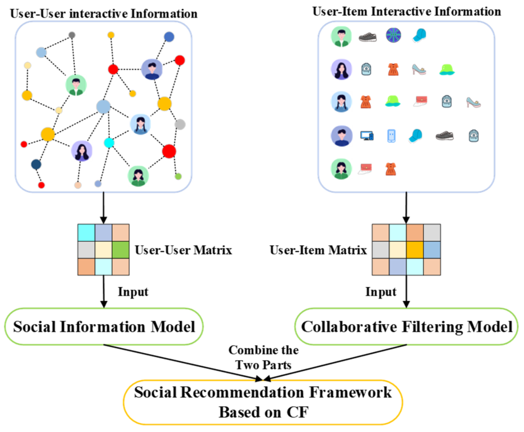
- Heterogeneous data are difficult to use: the data used in social recommendation often contain both user interaction data and user social data. Heterogeneity of data implies that we are in charge of handling representations of different objects (items and users); as a consequence, we deal with nodes which are not in the same embedded space, and, thus, these nodes are hard to be fused.
- (2)
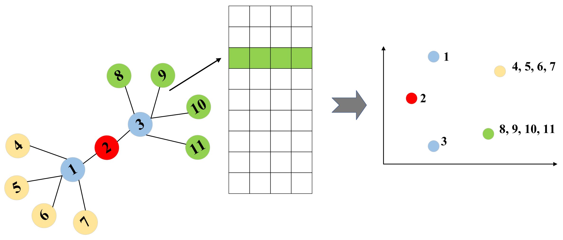
- High-order semantic information is hard to extract: For instance, high-order semantics describe relationships that users are indirectly connected to in the user–user social network. It is thus crucial to capture complex long-term dependencies between nodes. The more iteration layers of graph convolution architecture, the higher order semantic information will be extracted. However, excessive iteration layers will cause excessive smoothness.
- (3)
- Difficulties in fusing multiple semantic information: Social recommender systems manage both social network and interactive graph and it also has the task that effectively integrate the information coming from both of these graphs is still open research.
1.3. Our Contributions
- (1)
- We innovatively integrate social relations into the training of graph convolution-based collaborative filtering recommendation method. Specifically, we propose a graph convolution collaborative filtering recommendation model integrating social relations (called SRGCF). The SRGCF model learns node embeddings by integrating high-order semantic information about social behaviors as well as interactions.
- (2)
- We propose a recommender algorithm (called SRRA) running on top of the SRGCF model. The SRRA algorithm models the high-order relations in interactive data and social data, respectively, fuses these two types of high-order semantic information at the same layer and then forms the final embeddings. Generated embeddings are finally used in recommendation task.
- (3)
- We experimentally compared the SRRA algorithm with baselines on a range of real-life and large datasets. Our experiments indicate the superiority of our model against baselines.
2. Related Work
2.1. Traditional CF Recommendation Algorithm
2.2. Social Recommendation Algorithm
2.3. Graph Embedding Based Recommendation
3. Preliminaries
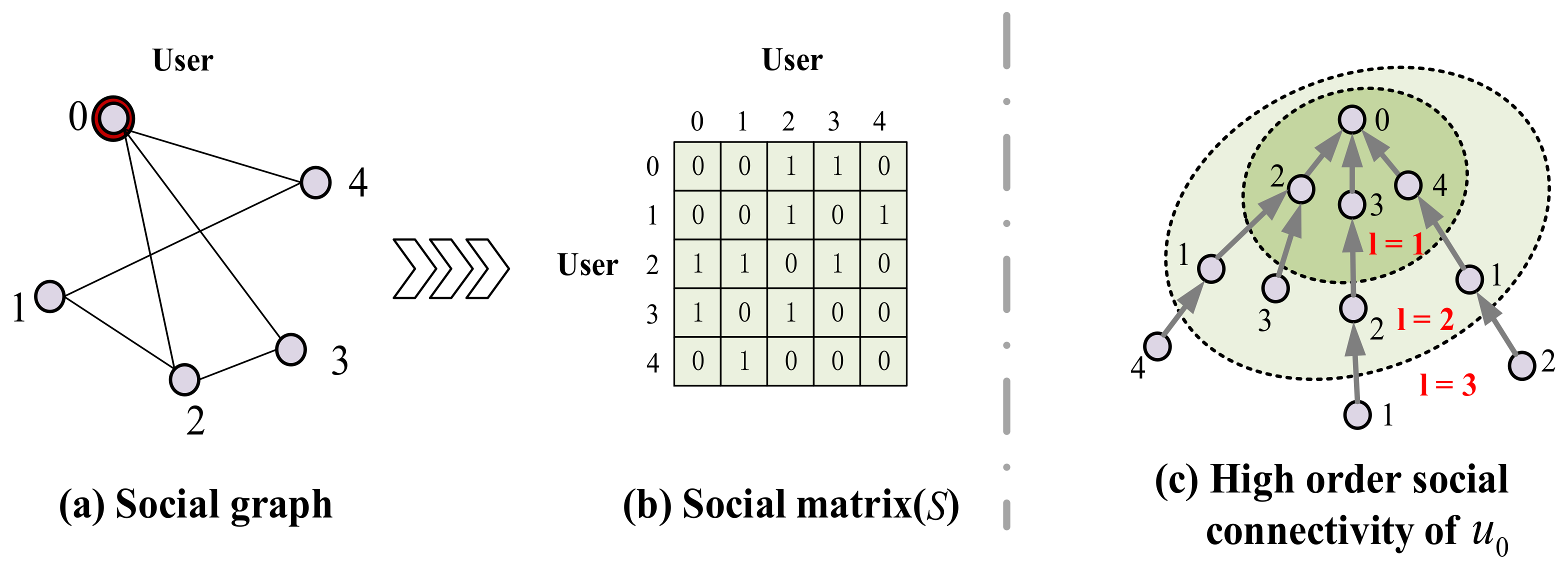
3.1. Social High-Order Connectivity
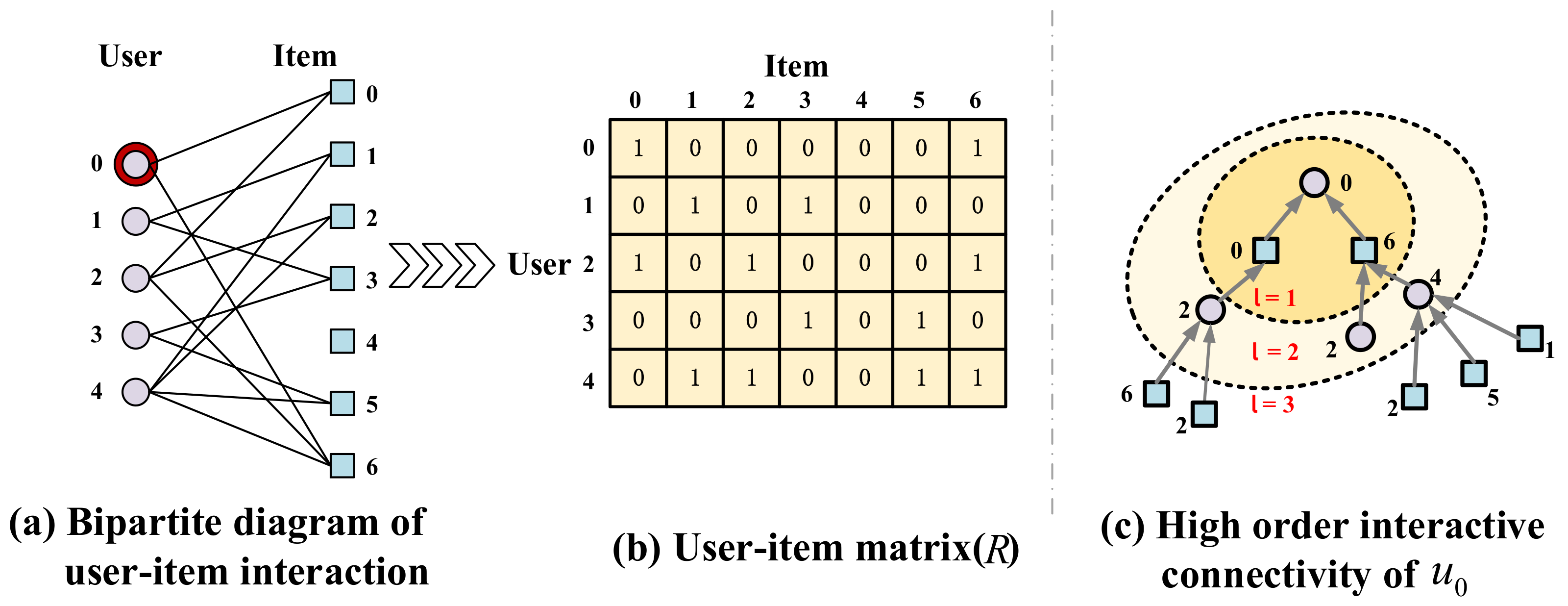
3.2. Interactive High-Order Connectivity
4. Proposed Recommendation Method
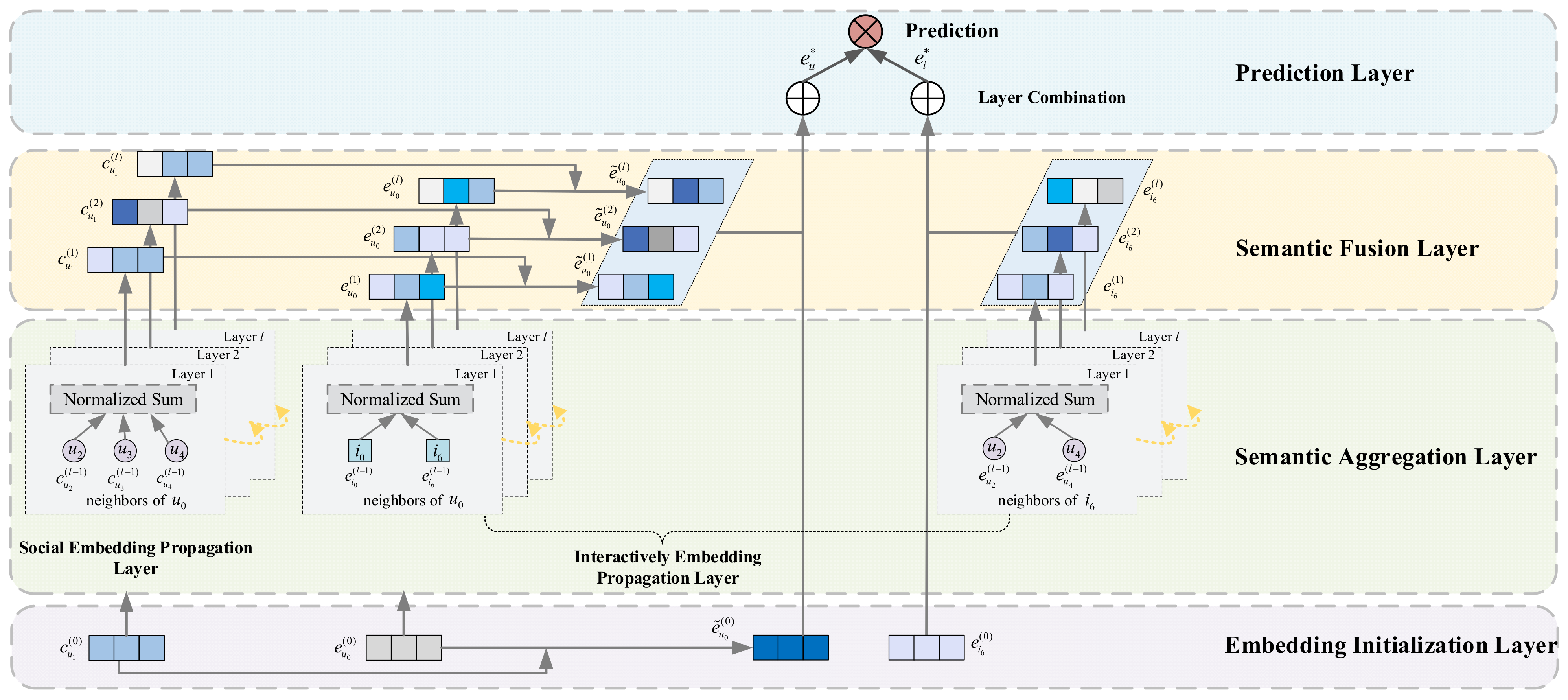
4.1. Recommendation Model Design
4.1.1. Embedding Initialization Layer
4.1.2. Semantic Aggregation Layer
- (1)
- First-order Semantic Aggregation
- (2)
- High-order Semantic Aggregation
- (a)
- Semantic Aggregation for SEPL
- (b)
- Semantic Aggregation for IEPL
4.1.3. Semantic Fusion Layer
4.1.4. Prediction Layer
4.2. The Proposed SRRA Recommendation Algorithm
| Algorithm 1: Social Relationship Recommendation Algorithm (SRRA). |
| Step1: calculate the embeddings of users and items |
| Input: R, S, M, N, d, l |
| Initialize: |
| calculate A and B by R, S, respectively |
| calculate D and P by A, B, respectively |
| , |
| For: |
| , respectively |
| , respectively |
| End For |
| Step2: calculate the loss of SRRA |
| For: |
| // add the regularization item into loss |
| For : // iterate over the positive example item set for user u |
| // calculate the score of positive samples |
| For : // iterate over the negative example item set for user u |
| // calculate the BPR loss |
| End For |
| End For |
| Step3: generate recommendations |
| Train the algorithm until it converges |
| According to the predicted score, select Top 10 items for recommendation |
| Return Recall, NDCG |
4.3. Model Training
5. Experiment
5.1. Experiment Setup
5.1.1. Datasets
- Brightkite. A position sharing platform with social networking platform where users share their locations through check-ins. It includes check-in data as well as social data.
- Gowalla. A position sharing platform similar to Brightkite. This dataset includes check-in data and user social data.
- Epinions. A consumer review website which allows users to clicked items and add trust users. This dataset contains users’ rating data and trust network data.
- LastFM. A social music platform for music sharing. This dataset includes data about users’ listening to music and users’ relationships.
5.1.2. Baselines
- LightGCN [3]: It is effective to extract the collaborative signal explicitly in the embedding process by modeling high-order connectivity in interactive graphs.
- DSCF [34]: It utilizes information provided by distant neighbors and explicitly captures the neighbor’s different opinions towards items.
- DiffNet [25]: It is a GNN model which analyzes how users make their decisions based on recursive social diffusion.
- GraphRec [24]: It captures interactions and opinions in GR and it also models two graphs (e.g., GR and GS) and the strength of heterogeneity in a coherent way.
- DICER [30]: It models user and item by introducing high-order neighbor information, and draws the most relevant interactive information based on deep context.
5.1.3. Evaluation Metrics
5.1.4. Experiments Details
5.2. Overall Comparison
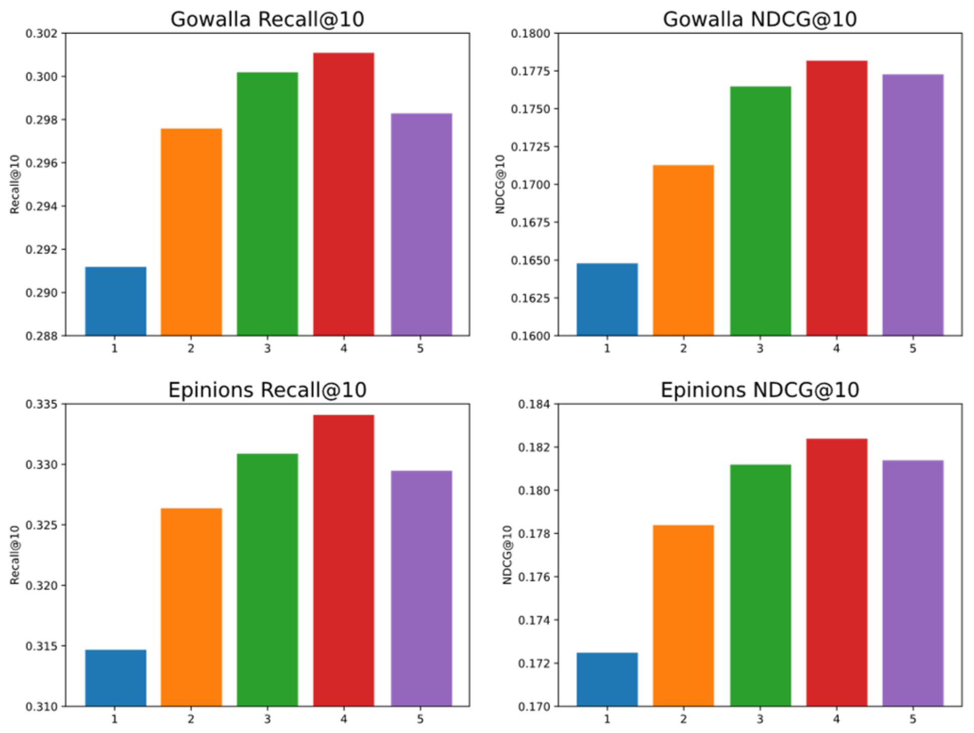
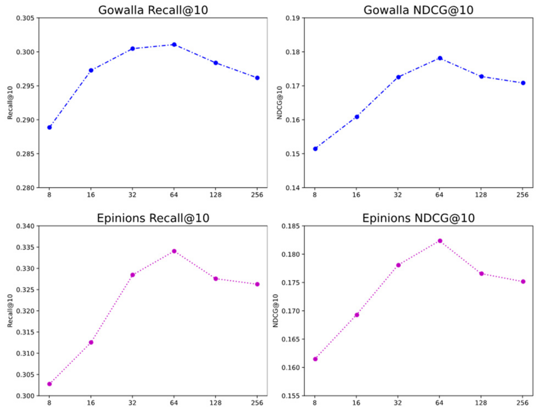
5.3. Parameter Analysis
6. Conclusions
Author Contributions
Funding
Institutional Review Board Statement
Informed Consent Statement
Data Availability Statement
Acknowledgments
Conflicts of Interest
Nomenclature
| U | the set of users |
| I | the set of items |
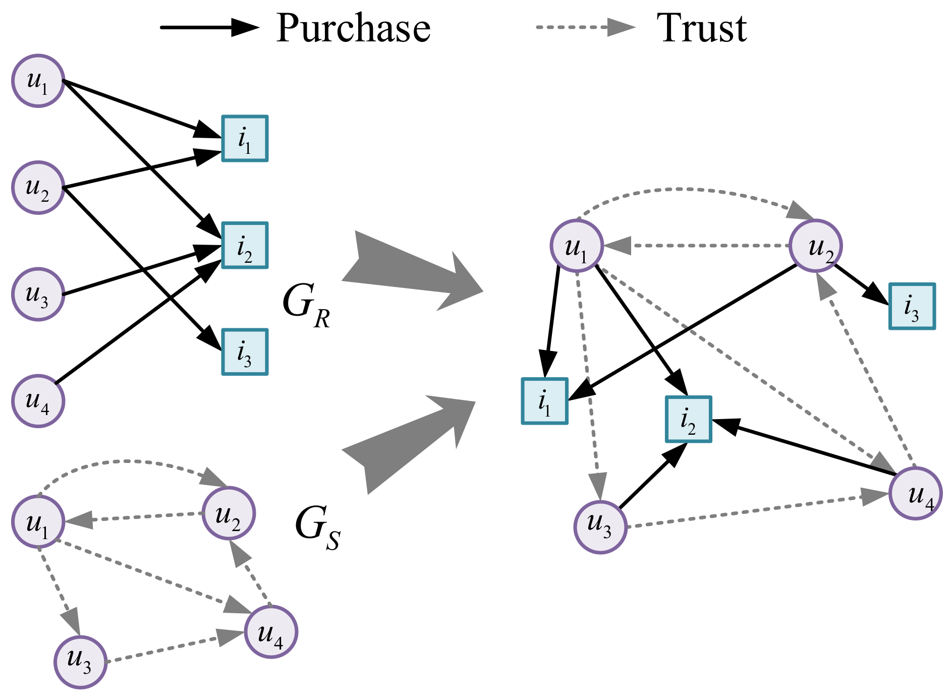
| GR | user–item interaction graph |
| Gs | user–user social graph |
| d | the dimension of node embedding |
| neighbors of item i on GR | |
| Hu | neighbors of user u on Gs |
| l | #layer |
| L | total number of layers |
| the friends of user u | |
| the embedding of user u at the l-th layer from GR | |
| the embedding of user u at the l-th layer from Gs | |
| the l-th layer embedding of user u from GR and Gs | |
| final embedding of user u | |
| final embedding of item i | |
| M | the numbers of users |
| N | the numbers of items |
| R | user–item interaction matrix |
| S | social matrix |
| A | adjacency matrix of GR |
| B | adjacency matrix of Gs |
| D | degree matrix of matrix A |
| P | degree matrix of matrix B |
| observable interactions | |
| unobserved interactions | |
| model parameters | |
| the l-th layer matrix of GCN on GR | |
| the l-th layer matrix of GCN on Gs | |
| final embedding matrix of users | |
| final embedding matrix of items |
References
- Liu, X.; Li, X.; Fiumara, G.; De Meo, P. Link prediction approach combined graph neural network with capsule network. Expert Syst. Appl. 2023, 212, 118737. [Google Scholar] [CrossRef]
- Liu, X.; Zhao, Z.; Zhang, Y.; Liu, C.; Yang, F. Social Network Rumor Detection Method Combining Dual-Attention Mechanism with Graph Convolutional Network. IEEE Trans. Comput. Soc. Syst. 2022. [Google Scholar] [CrossRef]
- He, X.; Deng, K.; Wang, X.; Li, Y.; Zhang, Y.; Wang, M. LightGCN: Simplifying and Powering Graph Convolution Network for Recommendation. In Proceedings of the 43rd International ACM SIGIR Conference on Research and Development in Information Retrieval (SIGIR’20), Virtual Event, 25–30 July 2020; pp. 639–648. [Google Scholar]
- Liu, T.; Deng, X.; He, Z.; Long, Y. TCD-CF: Triple cross-domain collaborative filtering recommendation. Pattern Recognit. Lett. 2021, 149, 185–192. [Google Scholar] [CrossRef]
- Nassar, N.; Jafar, A.; Rahhal, Y. A novel deep multi-criteria collaborative filtering model for recommendation system. Knowl. Based Syst. 2020, 187, 32–39. [Google Scholar] [CrossRef]
- He, X.; Liao, L.; Zhang, H.; Nie, L.; Hu, X.; Chua, T. Neural Collaborative Filtering. In Proceedings of the 26th International Conference on World Wide Web (WWW’17), Perth, Australia, 3–7 May 2017; pp. 173–182. [Google Scholar]
- Wang, H.; Wang, N.; Yeung, D. Collaborative Deep Learning for Recommender Systems. In Proceedings of the 21th ACM SIGKDD International Conference on Knowledge Discovery and Data Mining (KDD’15), Sydney, Australia, 10–13 August 2015; pp. 1235–1244. [Google Scholar]
- Xue, F.; He, X.; Wang, X.; Xu, J.; Liu, K.; Hong, R. Deep Item-based Collaborative Filtering for Top-N Recommendation. ACM Trans. Inf. Syst. 2019, 37, 1–25. [Google Scholar] [CrossRef] [Green Version]
- Khojamli, H.; Razmara, J. Survey of similarity functions on neighborhood-based collaborative filtering. Expert Syst. Appl. 2021, 185, 142–155. [Google Scholar] [CrossRef]
- Sanz-Cruzado, J.; Castells, P.; Macdonald, C.; Ounis, I. Effective contact recommendation in social networks by adaptation of information retrieval models. Inf. Process. Manag. 2020, 57, 1633–1647. [Google Scholar] [CrossRef]
- Sun, Z.; Guo, Q.; Yang, J.; Fang, H.; Guo, G.; Zhang, J.; Burke, R. Research commentary on recommendations with side information: A survey and research directions. Electron. Commer. Res. Appl. 2019, 37, 43–50. [Google Scholar] [CrossRef] [Green Version]
- Jamali, M.; Ester, M. A Matrix Factorization Technique with Trust Propagation for Recommendation in Social Networks. Assoc. Comput. Mach. 2010, 1, 135–142. [Google Scholar]
- Nitesh, C.; Wei, W. Collaborative User Network Embedding for Social Recommender Systems. In Proceedings of the 2017 SIAM International Conference on Data Mining, Sandy, UT, USA, 27–29 April 2017; pp. 381–389. [Google Scholar]
- Guibing, G.; Jie, Z.; Yorke, S.N. TrustSVD: Collaborative Filtering with Both the Explicit and Implicit Influence of User Trust and of Item Ratings. In Proceedings of the 29th AAAI Conference on Artificial Intelligence, New York, NY, USA; 2015; pp. 123–129. [Google Scholar]
- Ma, H.; Yang, H.; Lyu, M.R.; King, I. SoRec: Social Recommendation using Probabilistic Matrix Factorization. Neurocomputing 2019, 341, 931–940. [Google Scholar]
- Cui, P.; Wang, X.; Pei, J.; Zhu, W. A Survey on Network Embedding. IEEE Trans. Knowl. Data Eng. 2019, 31, 833–852. [Google Scholar] [CrossRef] [Green Version]
- Palash, G.; Emilio, F. Graph Embedding Techniques, Applications, and Performance: A Survey. Knowledge- Based Syst. 2017, 151, 78–84. [Google Scholar]
- Wang, D.; Cui, P.; Zhu, W. Structural Deep Network Embedding. In Proceedings of the 22nd ACM SIGKDD International Conference on Knowledge Discovery and Data Mining, San Francisco, CA, USA, 13–17 August 2016; pp. 1225–1234. [Google Scholar]
- Tang, J.; Qu, M.; Wang, M.; Zhang, M.; Yan, J.; Mei, Q. LINE: Large-scale Information Network Embedding. In Proceedings of the International Conference on World Wide Web, Florence, Italy, 18–22 May 2015; Volume 3, pp. 1067–1077. [Google Scholar]
- Perozzi, B.; Al-Rfou, R.; Skiena, S. Deepwalk: Online learning of social representations. In Proceedings of the 20th ACM SIGKDD International Conference on Knowledge Discovery and Data Mining, New York, NY, USA, 24–27 August 2014; pp. 701–710. [Google Scholar]
- Grover, A.; Leskovec, J. node2vec: Scalable Feature Learning for Networks. In Proceedings of the 22nd ACM SIGKDD International Conference on Knowledge Discovery and Data Mining (KDD’16), San Francisco, CA, USA, 13–17 August 2016; pp. 855–864. [Google Scholar]
- De Paola, A.; Gaglio, S.; Giammanco, A.; Lo Re, G.; Morana, M. A multi-agent system for itinerary suggestion in smart environments. CAAI Trans. Intell. Technol. 2021, 6, 377–393. [Google Scholar] [CrossRef]
- Weng, L.; Zhang, Q.; Lin, Z.; Wu, L. Harnessing heterogeneous social networks for better recommendations: A grey relational analysis approach. Expert Syst. Appl. 2021, 174, 142–154. [Google Scholar] [CrossRef]
- Fan, W.; Ma, Y.; Li, Q.; He, Y.; Zhao, Y.E.; Tang, J.; Yin, D. Graph Neural Networks for Social Recommendation. In Proceedings of the World Wide Web Conference (WWW 2019), San Francisco, CA, USA, 13–17 May 2019; pp. 417–426. [Google Scholar]
- Wu, L.; Sun, P.; Fu, Y.; Hong, R.; Wang, X.; Wang, M. A Neural Influence Diffusion Model for Social Recommendation. In Proceedings of the 42nd International ACM SIGIR Conference on Research and Development in Information Retrieval, SIGIR 2019, Paris, France, 21–25 July 2019; pp. 235–244. [Google Scholar]
- Yu, J.; Yin, H.; Li, J.; Wang, Q.; Hung, N.Q.V.; Zhang, X. Self-supervised multi-channel hypergraph convolutional network for social recommendation. In Proceedings of the Web Conference 2021, Ljubljana, Slovenia, 19–23 April 2021; pp. 413–424. [Google Scholar]
- Huang, C.; Xu, H.; Xu, Y.; Dai, P.; Xia, L.; Lu, M.; Bo, L.; Xing, H.; Lai, X.; Ye, Y. Knowledge-aware coupled graph neural network for social recommendation. In Proceedings of the 35th AAAI Conference on Artificial Intelligence (AAAI), Virtual, 2–9 February 2021. [Google Scholar]
- Wang, H.; Lian, D.; Tong, H.; Liu, Q.; Huang, Z.; Chen, E. HyperSoRec: Exploiting Hyperbolic User and Item Representations with Multiple Aspects for Social-aware Recommendation. ACM Trans. Inf. Syst. 2022, 40, 1–28. [Google Scholar] [CrossRef]
- Zhao, M.; Deng, Q.; Wang, K.; Wu, R.; Tao, J.; Fan, C.; Chen, L.; Cui, P. Bilateral Filtering Graph Convolutional Network for Multi-relational Social Recommendation in the Power-law Networks. ACM Trans. Inf. Syst. 2022, 40, 1–24. [Google Scholar] [CrossRef]
- Fu, B.; Zhang, W.; Hu, G.; Dai, X.; Huang, S.; Chen, J. Dual Side Deep Context-aware Modulation for Social Recommendation. In Proceedings of the Web Conference 2021, Ljubljana, Slovenia, 19–23 April 2021; pp. 2524–2534. [Google Scholar]
- Zhang, C.; Wang, Y.; Zhu, L.; Song, J.; Yin, H. Multi-graph heterogeneous interaction fusion for social recommendation. ACM Trans. Inf. Syst. TOIS 2021, 40, 1–26. [Google Scholar] [CrossRef]
- Rendle, S.; Freudenthaler, C.; Gantner, Z.; Schmidt-Thieme, L. BPR: Bayesian Personalized Ranking from Implicit Feedback. In Proceedings of the 25th Conference on Uncertainty in Artificial Intelligence, Montreal, QC, Canada, 18–21 June 2009; pp. 452–461. [Google Scholar]
- Kingma, D.P.; Ba, J.L. Adam: A Method for Stochastic Optimization. In Proceedings of the International Conference on Learning Representations, San Diego, CA, USA, 7–9 May 2015. [Google Scholar]
- Fan, W.; Ma, Y.; Yin, D.; Wang, J.; Tang, J.; Li, Q. Deep Social Collaborative Filtering. In Proceedings of the 13th ACM Conference on Recommender Systems (RecSys’19), Copenhagen, Denmark, 16–20 September 2019; pp. 305–313. [Google Scholar]


| Dataset | Brightkite | Gowalla | Epinions | LastFM |
|---|---|---|---|---|
| #User | 6310 | 14,923 | 12,392 | 1860 |
| #Item | 317,448 | 756,595 | 112,267 | 17,583 |
| #Interaction | 1,392,069 | 2,825,857 | 742,682 | 92,601 |
| #Connection | 27,754 | 82,112 | 198,264 | 24,800 |
| R-Density | 6.9495 × 10⁻⁴ | 2.5028 × 10⁻⁴ | 5.3384 × 10⁻⁴ | 2.8315 × 10⁻⁴ |
| S-Density | 6.9705 × 10⁻⁴ | 3.6872 × 10⁻⁴ | 1.2911 × 10⁻³ | 7.1685 × 10⁻³ |
| Methods | Social Recommendation | DL | Graph-Based | |
|---|---|---|---|---|
| GNN | GCN | |||
| LightGCN | √ | |||
| DSCF | √ | √ | ||
| DiffNet | √ | √ | √ | |
| GraphRec | √ | √ | √ | |
| DICER | √ | √ | √ | |
| SRRA | √ | √ | ||
| Recall@10 | |||||||
|---|---|---|---|---|---|---|---|
| Methods | LightGCN | DSCF | DiffNet | GraphRec | DICER | SRRA | |
| Datasets | |||||||
| Brightkite | 0.1642 | 0.1895 | 0.1962 | 0.2172 | 0.2235 | 0.2293 | |
| Gowalla | 0.2083 | 0.2253 | 0.2399 | 0.2779 | 0.2886 | 0.3011 | |
| Epinions | 0.2269 | 0.2613 | 0.2874 | 0.2845 | 0.3155 | 0.3341 | |
| LastFM | 0.2519 | 0.2742 | 0.2932 | 0.2876 | 0.3059 | 0.3272 | |
| NDCG@10 | |||||||
| Methods | LightGCN | DSCF | DiffNet | GraphRec | DICER | SRRA | |
| Datasets | |||||||
| Brightkite | 0.1321 | 0.1393 | 0.1539 | 0.1612 | 0.1672 | 0.1701 | |
| Gowalla | 0.1355 | 0.1482 | 0.1667 | 0.1724 | 0.1744 | 0.1782 | |
| Epinions | 0.1425 | 0.1598 | 0.1642 | 0.1709 | 0.1737 | 0.1824 | |
| LastFM | 0.1431 | 0.1563 | 0.1628 | 0.1862 | 0.1953 | 0.2086 | |
Publisher’s Note: MDPI stays neutral with regard to jurisdictional claims in published maps and institutional affiliations. |
© 2022 by the authors. Licensee MDPI, Basel, Switzerland. This article is an open access article distributed under the terms and conditions of the Creative Commons Attribution (CC BY) license (https://creativecommons.org/licenses/by/4.0/).
Share and Cite
Ma, M.; Cao, Q.; Liu, X. A Graph Convolution Collaborative Filtering Integrating Social Relations Recommendation Method. Appl. Sci. 2022, 12, 11653. https://doi.org/10.3390/app122211653
Ma M, Cao Q, Liu X. A Graph Convolution Collaborative Filtering Integrating Social Relations Recommendation Method. Applied Sciences. 2022; 12(22):11653. https://doi.org/10.3390/app122211653
Chicago/Turabian StyleMa, Min, Qiong Cao, and Xiaoyang Liu. 2022. "A Graph Convolution Collaborative Filtering Integrating Social Relations Recommendation Method" Applied Sciences 12, no. 22: 11653. https://doi.org/10.3390/app122211653