Entropy Optimization in MHD Nanofluid Flow over an Exponential Stretching Sheet

Abstract

We numerically investigate mixed convective heat and mass transport in incompressible nanofluid flow through an exponentially stretching sheet with temperature-dependent viscosity. The fluid flow equations are transformed to a system of non-linear ordinary differential equations using appropriate similarity transformations and solved numerically by using the multi-domain bivariate spectral quasi-linearization technique. The fast convergence of the method is shown by demonstrating that the error is exponentially small for a finite number of iterations. The significance and impact of different fluid parameters are presented and explained. For engineering relevance, the entropy generation number has been calculated for different fluid parameter values.

1. Introduction

Nanofluids are advanced heat transfer fluids with applications in a large variety of industrial processes. Over the last few years, the advancements in nanofluids have generated considerable research interest on account of their novel features that make them conceivably beneficial in a number of industrial processes, such as in glass blowing, cancer therapy, plastic and polymer extrusion, micro-forming, and air conditioning.

The potential benefits and challenges of using nanofluids with controlled particle characteristics for various heat transfer applications have been investigated by many researchers. In particular, the ion-slip effects on MHD flow, which find applications in nuclear power reactors, power generation, and in several areas of astrophysics and geophysics, have been studied by [1,2]. The MHD free-forced convective nanofluid fluid flow over a permeable medium was studied by Nadeem et al. [3]. The Casson nanofluid flow with entropy generation was investigated by Haq et al. [4]. Considering mixed convection on fluid flow is very significant for industrial applications, as free or forced convection may not be enough independently to disperse adequate thermal energy. Rehman et al. [5] examined the mixed convection in a water-based nanofluid in an MHD stagnation point flow. In physical flows, a magnetic field may have a significant impact on the flow of nanofluids. Fluid flow in electrical and magnetic fields may be used, for example, to control the cooling rate. Such an implementation has been analyzed by Makinde et al. [6].

A source of heat (or sink) in a flowing fluid is increasingly becoming important to researchers. These are important in manufacturing processes and other applications, which include nuclear waste disposal, storage of food, and exothermic processes in reactors. The effect of activation energy and an exponentially fluctuating temperature-dependent source in MHD heat transfer was investigated in [7,8,9,10].

A review of previous research shows that, when estimating the performance of thermal systems, heat irreversibility is unavoidable and remains at the core of these processes. The second law of thermodynamics is used in quantifying irreversibility in optimal thermal system design. The generation of entropy is a criterion for the non-optimal operation of a thermal system. Rashidi et al. [11] studied the generation of entropy in the flow of a convective nanofluid through a vertically expanding surface. Their research found that when the Brinkman number increased, so did the level of chaos in the system. Almakki et al. [12,13] presented the formulation for entropy generation in forced convection flow of radiative viscous nanofluids. Hosseinzadeh et al. [14] calculated the entropy optimization for a magnetized flow of a nanofluid with heat radiation. Aziz et al. [15] studied the volumetric entropy production in a non-Newtonian fluid passing a stretched surface with linear thermal radiation. More current relevant research addressing the optimization of entropy in the direction of a stretched surface with varied flow parameters may be found in Pal et al. [16] and the references therein.

The aim of the current study was to investigate entropy generation and the effect of the Bejan number on 2-dimensional MHD viscoelastic incompressible nanofluid flow through an exponentially expanding sheet. The influences of dominant factors such as fluid buoyancy, viscous dissipation, heat absorption, and heat generation were studied by Maleki et al. [17]. The flow over an impermeable surface in the presence of thermal radiation and viscous dissipation was analyzed by Sharma et al. [18]. There are currently many demands for heating and cooling processes using fluids containing metallic nanoparticles. To control the rate of heat transfer in the vicinity of the expanded lamina, both entropy and Bejan number play a key role. The governing partial differential equations (PDEs) are converted to non-linear ordinary differential equations (ODEs) and solved numerically using the multi-domain bivariate spectral quasi linearization technique (MD-BSQLM). Using the MD-BSQLM approach, the linearized equations are solved numerically.

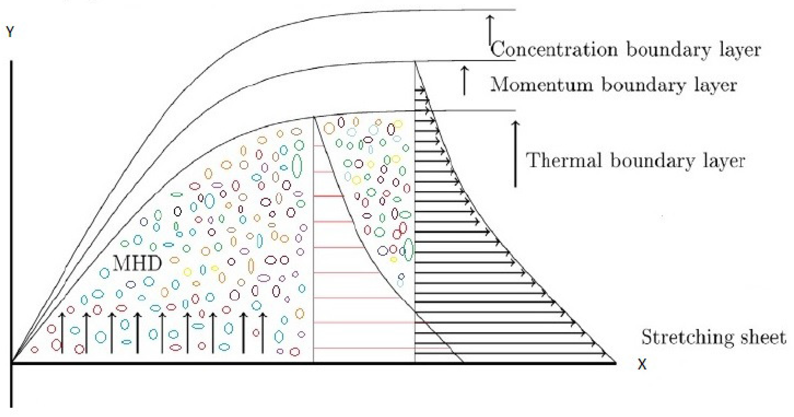
2. Problem Formulation

We investigated laminar free-forced convective mass-heat transportation along an exponentially stretching surface in viscous incompressible fluid in a magnetic field. We assumed that $u\to U_{\infty }=a{x}^m$ is the stretching velocity, where m is the stretching rate, $T_w$ is the temperature at the surface, and $T_{\infty }$ is the ambient temperature, where $T_w>T_{\infty }$. The magnetic field is aligned in y-direction to influence the velocity of the fluid, as shown in Figure 1.

The steady, incompressible fluid flow equations for a viscous nanofluid flow under these assumptions can be obtained as follows; see [19,20]:

$$\begin{array}{ccc}& & \frac{\partial u}{\partial x}+\frac{\partial v}{\partial y}=0,\hfill \end{array}$$

(1)

$$\begin{array}{ccc}& & u\frac{\partial u}{\partial x}+v\frac{\partial u}{\partial y}=\frac{1}{{\rho }_{\infty }}\frac{\partial }{\partial u}\left(\mu \frac{\partial u}{\partial y}\right)+\frac{\sigma B_0^2}{{\rho }_{\infty }}\left(U_{\infty }-u\right)+g{\beta }_T\left(T-T_{\infty }\right)+g{\beta }_C\left(C-C_{\infty }\right),\hfill \\ & & u\frac{\partial T}{\partial x}+v\frac{\partial T}{\partial y}=\alpha \frac{{\partial }^{2}T}{\partial y^2}+\frac{Q_0}{{\rho }_{\infty }{c}_p}\left(T-T_{\infty }\right)+\frac{16{\sigma }^{*}{T}_{\infty }^3}{3k^{*}{\rho }_{\infty }{c}_p}\frac{{\partial }^{2}T}{\partial y^2}+\frac{{\nu }_{\infty }}{c_p}{\left(\frac{\partial u}{\partial y}\right)}^2+\frac{\sigma B_0^2}{{\rho }_{\infty }{c}_p}{u}^2+\hfill \end{array}$$

(2)

$$\begin{array}{ccc}& & \tau \left[D_B\frac{\partial C}{\partial y}\frac{\partial T}{\partial y}+\frac{D_T}{T_{\infty }}{\left(\frac{\partial T}{\partial y}\right)}^2\right],\hfill \end{array}$$

(3)

$$\begin{array}{ccc}& & u\frac{\partial C}{\partial x}+v\frac{\partial C}{\partial y}=D_B\frac{{\partial }^{2}C}{\partial y^2}+\frac{D_T}{T_{\infty }}\frac{{\partial }^{2}T}{\partial y^2}-R_0\left(C-C_{\infty }\right),\end{array}$$

(4)

where u and v are the velocity components in x and y-directions, respectively; ${\rho }_{\infty },U_{\infty },T_{\infty }$, ${\nu }_{\infty }$, and $C_{\infty }$ represent the density, velocity, temperature, kinematic viscosity, and concentration of the fluid in free stream, respectively; $B_0$ is the external magnetic field applied in y-direction; g is the acceleration; ${\beta }_C$ and ${\beta }_T$ are the concentration and thermal expansions, respectively; $\alpha$ represents the thermal diffusion; $Q_0$ represents the heat generation rate; $k^{*}$ is the mean absorption coefficient; $c_p$ is the specific heat of nanoparticles; ${\sigma }^{*}$ represents the Stefan Boltzmann constant; $\sigma$ and $\tau$ are the electrical conductivity and ratio of nanoparticle heat capacity, respectively; $D_B$ is the Brownian mention; T and C are the temperature and concentration distributions of the fluid, respectively; $R_0$ is a chemical reaction parameter; $D_T$ represents the thermophoretic diffusion coefficient.

The auxiliary conditions are

$$\begin{array}{ccc}& & u=0,vs.=0,T=T_{\infty },C=C_{\infty }\mathrm{at}y=0,\hfill \\ & & u\to U_{\infty }=a{x}^m,T\to T_{\infty },C\to C_{\infty }\mathrm{at}y\to \infty .\hfill \end{array}$$

(5)

Equations (1)–(4) may be simplified using the variables [19]

$$\begin{array}{ccc}& & \psi ={{\displaystyle (}x{U}_{\infty }{\nu }_{\infty }{\displaystyle )}}^{1/2}f(\eta ,\xi ),\eta =y{\left(\frac{U_{\infty }}{x{\nu }_{\infty }}\right)}^{1/2},\xi =\frac{\sigma B_0^2}{{\rho }_{\infty }{U}_{\infty }}x,\hfill \\ & & \mu ={\mu }_0{e}^{-{\beta }_1\theta (\eta ,\xi )},\theta (\eta ,\xi )=\frac{T-T_{\infty }}{T_w-T_{\infty }},h(\eta ,\xi )=\frac{C-C_{\infty }}{C_w-C_{\infty }}.\hfill \end{array}$$

(6)

Using these transformations, continuity is satisfied and Equations (2)–(4) are reduced to the following equations, where the velocity, temperature, and concentration fields are denoted by $f^{\prime }(\eta ,\xi )$, $\theta (\eta ,\xi )$, and $h(\eta ,\xi )$, respectively:

$$\begin{array}{ccc}& & f^{‴}-{\beta }_1{f}^{″}{\theta }^{\prime }+\frac{1}{2}{e}^{{\beta }_1\theta }f{f}^{″}+e^{{\beta }_1\theta }{\displaystyle [}\xi {\displaystyle (}1-f^{\prime }{\displaystyle )}+G{r}_T\theta +G{r}_{C}h{\displaystyle ]}=\xi e^{{\beta }_1\theta }\left[f^{\prime }\frac{\partial f^{\prime }}{\partial \xi }-f^{″}\frac{\partial f}{\partial \xi }\right],\hfill \end{array}$$

(7)

$$\begin{array}{ccc}& & \frac{1+Nr}{Pr}{\theta }^{″}+\frac{1}{2}f{\theta }^{\prime }+\lambda \xi \theta +Ec{\displaystyle [}{f}^{{″}^2}+\xi f^{{\prime }^2}{\displaystyle ]}+Nb{h}^{\prime }{\theta }^{\prime }+Nt{\theta }^{{\prime }^2}=\xi \left[f^{\prime }\frac{\partial \theta }{\partial \xi }-{\theta }^{\prime }\frac{\partial f}{\partial \xi }\right],\hfill \end{array}$$

(8)

$$\begin{array}{ccc}& & h^{″}+Le\frac{1}{2}f{h}^{\prime }+\frac{Nt}{Nb}{\theta }^{″}-Le{R}_{1}h=Le\xi \left[f^{\prime }\frac{\partial h}{\partial \xi }-h^{\prime }\frac{\partial f}{\partial \xi }\right].\hfill \end{array}$$

(9)

In Equations (7)–(9), the parameters are given by

$$\begin{array}{ccc}& & G{r}_T={\displaystyle \frac{g{\beta }_T(T_w-T_{\infty })x/{\nu }_{\infty }^2}{U_{\infty }^2{\nu }_{\infty }^2}},G{r}_C={\displaystyle \frac{g{\beta }_C(C_w-C_{\infty })x/{\nu }_{\infty }^2}{U_{\infty }^2{\nu }_{\infty }^2}},Nr={\displaystyle \frac{16{\sigma }^{*}{T}_{\infty }^3}{3k^{*}{k}_f}},\hfill \\ & & Pr={\displaystyle \frac{{\nu }_{\infty }}{\tau }},\lambda ={\displaystyle \frac{Q_0}{\sigma B_0^2{c}_p}},Ec={\displaystyle \frac{U_{\infty }}{(T_w-T_{\infty })c_p}},\hfill \\ & & Nb={\displaystyle \frac{\tau (C_w-C_{\infty })D_B}{{\nu }_{\infty }}},Le={\displaystyle \frac{{\nu }_{\infty }}{D_B}},Nt={\displaystyle \frac{\tau (T_w-T_{\infty })D_T}{T_{\infty }{\nu }_{\infty }}},R_1={\displaystyle \frac{R_{0}x}{U_{\infty }}},\hfill \end{array}$$

where $G{r}_T$ and $G{r}_C$ are the Grashof numbers for temperature and concentration, respectively; $Nr$ is the thermal radiation parameter; $Nt$ is the thermophoresis parameter; $Pr$ and $Ec$ are the Prandtl and Eckert numbers; $\lambda$ is the heat generation (dimensionless); $Nb$ represents the Brownian motion parameter; and $R_1$ is the chemical reaction parameter.

The transformed boundary conditions are

$$\begin{array}{ccc}& & f(0,\xi )=0,f^{\prime }(0,\xi )=0,\theta (0,\xi )=1,h(0,\xi )=1,\hfill \\ & & f^{\prime }(\infty ,\xi )=1,\theta (\infty ,\xi )=0,h(\infty ,\xi )=0,\hfill \end{array}$$

(10)

where the prime denotes the derivative with respect to $\eta$.

The important physical parameters for this flow with heat and mass transfer situations are the local skin-friction coefficient, the local Nusselt number, and the local Sherwood number, which can be defined as:

$$\begin{array}{ccc}& & C{f}_x=2R{e}_x^{-1/2}{f}^{″}(\xi ,0),N{u}_x=-R{e}_x^{1/2}(1+Nr){\theta }^{\prime }(\xi ,0),S{h}_x=-R{e}_x^{1/2}{h}^{\prime }(\xi ,0),\hfill \end{array}$$

(11)

where $R{e}_x$ is the local Reynolds number in x-direction.

3. Entropy Generation Analysis

The principal contributors to irreversibilities in the fluid include the heat transfer through thermal radiation, viscous dissipation, magnetic field, and mass transfer, respectively.

The volumetric rate of the entropy generation rate is written as (see [21,22])

$$\begin{array}{ccc}& & S_{gen}^{‴}=\underset{\mathrm{heat\; transfer}}{\underbrace{\frac{1}{T_{\infty }^2}\left[k_f+\frac{16{\sigma }^{*}{T}_{\infty }^3}{3k^{*}}\right]{\left(\frac{\partial T}{\partial y}\right)}^2}}+\underset{\mathrm{viscous\; dissipation}}{\underbrace{\frac{\mu }{T_{\infty }}{\left(\frac{\partial u}{\partial y}\right)}^2}}+\underset{\mathrm{magnetic\; field}}{\underbrace{\frac{\sigma B_0^2}{T_{\infty }}{u}^2}}+\hfill \\ & & \underset{\mathrm{mass\; transfer}}{\underbrace{\frac{RD}{C_{\infty }}\left[{\left(\frac{\partial C}{\partial x}\right)}^2+{\left(\frac{\partial C}{\partial y}\right)}^2\right]+\frac{RD}{T_{\infty }}\left[\left(\frac{\partial T}{\partial x}\right)\left(\frac{\partial C}{\partial x}\right)+\left(\frac{\partial T}{\partial y}\right)\left(\frac{\partial C}{\partial y}\right)\right]}}.\hfill \end{array}$$

(12)

We define $S_0^{‴}$ as the dimensionless entropy generation rate—see [12,23]—such that

$$\begin{array}{ccc}& & S_0^{‴}=\frac{k_f{\left(T_w-T_{\infty }\right)}^2}{T_{\infty }^2{x}^2}.\hfill \end{array}$$

(13)

The rate of entropy generation can be expressed as

$$\begin{array}{ccc}\hfill & & N_G(\eta ,\xi )=\frac{S_{gen}^{‴}}{S_0^{‴}}=Re\left(1+Nr\right){\theta }^{{\prime }^2}+\frac{ReBr}{\Omega }\xi f^{{\prime }^2}+\Sigma {\left(\frac{\chi }{\Omega }\right)}^2[\left(Re+\frac{{\eta }^2}{4}\right)h^{{\prime }^2}-\eta \xi h^{\prime }\frac{\partial h}{\partial \xi }+\hfill \\ & & {\xi }^2{\left(\frac{\partial h}{\partial \xi }\right)}^2]+\Sigma \frac{\chi }{\Omega }\left[\left(Re+\frac{{\eta }^2}{4}\right){\theta }^{\prime }{h}^{\prime }+{\xi }^2\frac{\partial \theta }{\partial \xi }\frac{\partial h}{\partial \xi }-\frac{\eta \xi }{2}\left({\theta }^{\prime }\frac{\partial h}{\partial \xi }+h^{\prime }\frac{\partial \theta }{\partial \xi }\right)\right]+\frac{ReBr}{\Omega }{e}^{-{\beta }_1\theta }{f}^{{″}^2}.\hfill \end{array}$$

(14)

The parameters appearing in Equation (14) are defined as

$$\begin{array}{ccc}& & Re=\frac{U_{\infty }\left(x\right)x}{{\nu }_{\infty }},Br=\frac{{\mu }_{\infty }{U}_{\infty }^2}{k_f\Delta T},\Omega =\frac{\Delta T}{T_{\infty }}=\frac{T_w-T_{\infty }}{T_{\infty }},\hfill \\ & & \Sigma =\frac{C_{\infty }RD}{k_f},\chi =\frac{C_w-C_{\infty }}{C_{\infty }},\hfill \end{array}$$

(15)

where $Re$ is the local Reynolds number, $Br$ is the Brinkman number, $\Omega$ is the temperature difference, $\Sigma$ is the dimensionless parameter, $\chi$ and R are the diffusion parameter and universal gas constant, respectively, and D is the mass diffusion.

4. Method of Solution

4.1. Multi-Domain Bivariate Spectral Quasi-Linearization Method (MD-BSQLM)

The non-linear dimensionless ordinary differential equations were solved numerically to a high level of accuracy using the MD-BSQLM [24]. In [25,26], the method was used to solve equations describing the mixed convection flow of the power law and Casson nanofluids. We use the method to solve the nonlinear system of differential Equations (7)–(9), where we apply the multi-domain approach in the $\xi$-direction only. To use the multi-domain concept, let $\xi \in \Lambda$, where $\Lambda =[0,T]$, and consider the subdivisions

$$\begin{array}{c}\hfill {\Lambda }_m=[{\xi }_{m-1},{\xi }_m],m=1,2,\cdots ,p\mathrm{with}0={\xi }_0<{\xi }_1<{\xi }_2<\cdots <{\xi }_p=T.\end{array}$$

(16)

If the solutions to Equations (7)–(9) are denoted by $f^{\left(m\right)}({\xi }_{\left(m\right)},\eta )$, ${\theta }^{\left(m\right)}({\xi }_{\left(m\right)},\eta )$ and $h^{\left(m\right)}({\xi }_{\left(m\right)},\eta )$, respectively, then in the first interval $[{\xi }_0,{\xi }_1]$, the solutions

$$\begin{array}{c}\hfill f^{\left(1\right)}(\xi ,\eta ),{\theta }^{\left(1\right)}(\xi ,\eta ),h^{\left(1\right)}(\xi ,\eta ),\end{array}$$

(17)

are obtained subject to the “initial” conditions

$$\begin{array}{c}\hfill f^{\left(1\right)}(0,\eta ),{\theta }^{\left(1\right)}(0,\eta ),h^{\left(1\right)}(0,\eta ).\end{array}$$

(18)

In each interval $[{\xi }_{m-1},{\xi }_m]$, ($m\ge 2$), the continuity conditions

$$\begin{array}{c}{f}^{\left(m\right)}({\xi }_{m-1},\eta )=f^{(m-1)}({\xi }_{m-1},\eta ),\\ {\theta }^{\left(m\right)}({\xi }_{m-1},\eta )={\theta }^{(m-1)}({\xi }_{m-1},\eta ),\\ h^{\left(m\right)}({\xi }_{m-1},\eta )=h^{(m-1)}({\xi }_{m-1},\eta ),\end{array}$$

(19)

hold. This process is repeated to generate a sequence of solutions

$$\begin{array}{c}\hfill f^{\left(m\right)}(\xi ,\eta ),{\theta }^{\left(m\right)}(\xi ,\eta ),h^{\left(m\right)}(\xi ,\eta ).\end{array}$$

(20)

In the next step, we linearize the nonlinear system of Equations (7)–(9).

4.2. Linearization

The non-linear terms in Equations (7)–(9) are converted into a recursive sequence with linear components; see [27,28,29].

Applying the QLM technique to Equations (7)–(9) gives the following:

$$\begin{array}{c}{f}_{e+1}^{{}^{‴}\left(m\right)}+a_{1,e}{f}_{e+1}^{{}^{″}\left(m\right)}+a_{2,e}{f}_{e+1}^{{}^{\prime }\left(m\right)}+a_{3,e}{f}_{e+1}^{\left(m\right)}+a_{4,e}\frac{\partial f_{e+1}^{{}^{\prime }\left(m\right)}}{\partial \xi }+a_{5,e}\frac{\partial f_{e+1}^{\left(m\right)}}{\partial \xi }+a_{6,e}{\theta }_{e+1}^{{}^{\prime }\left(m\right)}+a_{7,e}{\theta }_{e+1}^{\left(m\right)}+a_{8,e}{h}_{e+1}^{\left(m\right)}=R_{1,e},\hfill \\ b_{0,e}{\theta }_{e+1}^{{}^{″}\left(m\right)}+b_{1,e}{\theta }_{e+1}^{{}^{\prime }\left(m\right)}+b_{2,e}{\theta }_{e+1}^{\left(m\right)}+b_{3,e}\frac{\partial {\theta }_{e+1}^{\left(m\right)}}{\partial \xi }+b_{4,e}{f}_{e+1}^{{}^{″}\left(m\right)}+b_{5,e}{f}_{e+1}^{{}^{\prime }\left(m\right)}+b_{6,e}{f}_{e+1}^{\left(m\right)}+b_{7,e}\frac{\partial f_{e+1}^{\left(m\right)}}{\partial \xi }+b_{8,e}{h}_{e+1}^{{}^{\prime }\left(m\right)}=R_{2,e},\hfill \\ h_{e+1}^{{}^{″}\left(m\right)}+c_{1,e}{h}_{e+1}^{{}^{\prime }\left(m\right)}+c_{2,e}{h}_{e+1}^{\left(m\right)}+c_{3,e}\frac{\partial h_{e+1}^{\left(m\right)}}{\partial \xi }+c_{4,e}{f}_{e+1}^{{}^{\prime }\left(m\right)}+c_{5,e}{f}_{e+1}^{\left(m\right)}+c_{6,e}\frac{\partial f_{e+1}^{\left(m\right)}}{\partial \xi }+c_{7,e}{\theta }_{e+1}^{{}^{″}\left(m\right)}=R_{3,e},\hfill \end{array}$$

(21)

where the variable coefficients $a_{i,e},b_{i,e},c_{i,e}$ and $d_{i,e}(i=1,2,3,\dots )$ are presumed to be known from previous calculations and are given by

$$\begin{array}{ccc}& & a_{1,e}=-{\beta }_1{\theta }_e^{\prime }+\frac{1}{2}{e}^{{\beta }_1{\theta }_e}{f}_e+\xi e^{{\beta }_1{\theta }_e}\frac{\partial f_e}{\partial \xi },a_{2,e}=-\xi e^{{\beta }_1{\theta }_e}\left(1+\frac{\partial f_e^{\prime }}{\partial \xi }\right),a_{3,e}=\frac{1}{2}{e}^{{\beta }_1{\theta }_e}{f}_e^{″},a_{4,e}=-\xi e^{{\beta }_1{\theta }_e}{f}_e^{\prime },\hfill \\ & & a_{5,e}=\xi e^{{\beta }_1{\theta }_e}{f}_e^{″},a_{6,e}=-{\beta }_1{f}_e^{″},a_{7,e}={\beta }_1{e}^{{\beta }_1{\theta }_e}\left[\frac{1}{2}{f}_e{f}_e^{″}+\xi (1-f^{\prime })+G{r}_T{\theta }_e+G{r}_C{h}_e-f_e^{\prime }\frac{\partial f_e^{\prime }}{\partial \xi }+f_e^{″}\frac{\partial f_e}{\partial \xi }+\frac{G{r}_T}{{\beta }_1}\right],\hfill \\ & & a_{8,e}=e^{{\beta }_1{\theta }_e}G{r}_C,\hfill \\ & & b_{0,e}=\frac{1+Nr}{Pr},b_{1,e}=\frac{1}{2}{f}_e^{\left(m\right)}+N_b{h}_e^{{}^{\prime }\left(m\right)}+2N_t{\theta }_e^{{}^{\prime }\left(m\right)}+\xi \frac{\partial f_e^{\left(m\right)}}{\partial \xi },b_{2,e}=\lambda \xi ,b_{3,e}=-\xi f_e^{{}^{\prime }\left(m\right)},b_{4,e}=2Ec{f}_e^{{}^{″}\left(m\right)},\hfill \\ & & b_{5,e}=2\xi Ec{f}_e^{{}^{\prime }\left(m\right)}-\xi \frac{\partial {\theta }_e^{\left(m\right)}}{\partial \xi },b_{6,e}=\frac{1}{2}{\theta }_e^{{}^{\prime }\left(m\right)},b_{7,e}=\xi {\theta }_e^{{}^{\prime }\left(m\right)},b_{8,e}=N_b{\theta }_e^{{}^{\prime }\left(m\right)},\hfill \\ & & c_{1,e}=\frac{1}{2}Le{f}_e^{\left(m\right)}+Le\xi \frac{\partial f_e^{\left(m\right)}}{\partial \xi },c_{2,e}=-Le{R}_1,c_{3,e}=-Le\xi f_e^{{}^{\prime }\left(m\right)},\hfill \\ & & c_{4,e}=-Le\xi \frac{\partial h_e^{\left(m\right)}}{\partial \xi },c_{5,e}=\frac{1}{2}Le{h}_e^{{}^{\prime }\left(m\right)},c_{6,e}=Le\xi h_e^{{}^{\prime }\left(m\right)},c_{7,e}=\frac{N_t}{N_b}.\hfill \end{array}$$

Here, the right-hand side terms $R_{i,e}(i=1,2,3)$ in Equation (23) are given below:

$$\begin{array}{c}{R}_{1,e}=f_e^{{}^{‴}\left(m\right)}+a_{1,e}{f}_e^{{}^{″}\left(m\right)}+a_{2,e}{f}_e^{{}^{\prime }\left(m\right)}+a_{3,e}{f}_e^{\left(m\right)}+a_{4,e}\frac{\partial f_e^{\prime \left(m\right)}}{\partial \xi }+a_{5,e}\frac{\partial f_e^{\left(m\right)}}{\partial \xi }+a_{6,e}{\theta }_e^{{}^{\prime }\left(m\right)}+a_{7,e}{\theta }_e^{\left(m\right)}+a_{8,e}{h}_e^{\left(m\right)}-F_f,\hfill \\ R_{2,e}=b_{0,e}{\theta }_e^{{}^{″}\left(m\right)}+b_{1,e}{\theta }_e^{{}^{\prime }\left(m\right)}+b_{2,e}{\theta }_e^{\left(m\right)}+b_{3,e}\frac{\partial {\theta }_e^{\left(m\right)}}{\partial \xi }+b_{4,e}{f}_e^{{}^{″}\left(m\right)}+b_{5,e}{f}_e^{{}^{\prime }\left(m\right)}+b_{6,e}{f}_e^{\left(m\right)}+b_{7,e}\frac{\partial f_e^{\left(m\right)}}{\partial \xi }+b_{8,e}{h}_e^{{}^{\prime }\left(m\right)}-F_{\theta },\hfill \\ R_{3,e}=h_e^{{}^{″}\left(m\right)}+c_{1,e}{h}_e^{{}^{\prime }\left(m\right)}+c_{2,e}{h}_e^{\left(m\right)}+c_{3,e}\frac{\partial h_e^{\left(m\right)}}{\partial \xi }+c_{4,e}{f}_e^{{}^{\prime }\left(m\right)}+c_{5,e}{f}_e^{\left(m\right)}+c_{6,e}\frac{\partial f_e^{\left(m\right)}}{\partial \xi }+c_{7,e}{\theta }_e^{{}^{″}\left(m\right)}-F_h,\hfill \end{array}$$

(22)

and the functions $F_f,F_{\theta }$, and $F_h$ are as defined in Equations (7)–(9).

4.3. Collocation

The interval $\xi \in {\Lambda }_m\equiv [{\xi }_{m-1},{\xi }_m]$ is transformed to $s\in [-1,1]$ using the linear transformation

$$\xi =\frac{1}{2}({\xi }_m-{\xi }_{m-1})s+\frac{1}{2}({\xi }_m+{\xi }_{m-1}),$$

and $\eta \in [0,\infty ]$ is transformed to $x\in [-1,1]$ using

$$\eta =\frac{1}{2}L(x+1)$$

where L is a number large enough to represent the condition at infinity. For collocation, we use the Gauss–Lobatto collocation points defined as

$$x_i=cos\left(\frac{\pi i}{N_x}\right),s_j=cos\left(\frac{\pi j}{N_s}\right),i=0,1,\dots ,N_x,j=0,1,\dots ,N_s.$$

The Chebyshev differentiation matrix is as defined in [30], with respect to $\zeta$. The general form can be expressed as

$$\begin{array}{c}{\left.\frac{{\partial }^n{f}^{\left(m\right)}}{\partial x^n}\right|}_{(s_j,x_i)}={\mathbf{D}}^n{F}_i^{\left(m\right)},{\left.\frac{\partial f^{\left(m\right)}}{\partial s}\right|}_{(s_j,x_i)}=\sum _{q=0}^{Ns}{\mathbf{d}}_{iq}^{\left(m\right)}{F}_q^{\left(m\right)},\hfill \\ {\left.\frac{{\partial }^n{\theta }^{\left(m\right)}}{\partial x^n}\right|}_{(s_j,x_i)}={\mathbf{D}}^n{T}_i^{\left(m\right)},{\left.\frac{\partial {\theta }^{\left(m\right)}}{\partial s}\right|}_{(s_j,x_i)}=\sum _{q=0}^{Ns}{\mathbf{d}}_{iq}^{\left(m\right)}{T}_q^{\left(m\right)},\hfill \\ {\left.\frac{{\partial }^n{h}^{\left(m\right)}}{\partial x^n}\right|}_{(s_j,x_i)}={\mathbf{D}}^n{H}_i^{\left(m\right)},{\left.\frac{\partial h^{\left(m\right)}}{\partial s}\right|}_{(s_j,x_i)}=\sum _{q=0}^{Ns}{\mathbf{d}}_{iq}^{\left(m\right)}{H}_q^{\left(m\right)},i=0,1,\dots ,Nx,\hfill \end{array}$$

(23)

where

$$\begin{array}{ccc}& & F_i={[f(s_j,x_0),f(s_j,x_1),\dots ,f(s_j,x_{Nx})]}^T,T_i={[\theta (s_j,x_0),\theta (s_j,x_1),\dots ,\theta (s_j,x_{Nx})]}^T,\hfill \\ & & H_i={[h(s_j,x_0),h(s_j,x_1),\dots ,h(s_j,x_{Nx})]}^T,\mathbf{d}=\frac{2d}{{\zeta }_m-{\zeta }_{m-1}},\mathbf{D}=\frac{2D}{C}.\hfill \end{array}$$

By applying Equations (21)–(23), we obtain

$$\begin{array}{c}\left({\mathbf{D}}^3+{\mathbf{a}}_{\mathbf{1},\mathbf{e}}{\mathbf{D}}^2+{\mathbf{a}}_{\mathbf{2},\mathbf{e}}\mathbf{D}+{\mathbf{a}}_{\mathbf{3},\mathbf{e}}I+{\mathbf{a}}_{\mathbf{4},\mathbf{e}}{\mathbf{d}}_{ii}^{\left(m\right)}\left(\mathbf{D}\right)+{\mathbf{a}}_{\mathbf{5},\mathbf{e}}{\mathbf{d}}_{ii}^{\left(m\right)}I\right)F_{i,e+1}^{\left(m\right)}\hfill \\ +\left({\mathbf{a}}_{\mathbf{4},\mathbf{e}}\sum _{\begin{array}{c}q=0\\ q\ne i\end{array}}^{Ns-1}{\mathbf{d}}_{iq}^{\left(m\right)}\left(\mathbf{D}\right)+{\mathbf{a}}_{\mathbf{5},\mathbf{e}}\sum _{\begin{array}{c}q=0\\ q\ne i\end{array}}^{Ns-1}{\mathbf{d}}_{iq}^{\left(m\right)}I\right)F_{q,e+1}^{\left(m\right)}+\left({\mathbf{a}}_{\mathbf{6},\mathbf{e}}\mathbf{D}+{\mathbf{a}}_{\mathbf{7},\mathbf{e}}I\right)T_{i,e+1}^{\left(m\right)}\hfill \\ +{\mathbf{a}}_{\mathbf{8},\mathbf{e}}{H}_{i,e+1}^{\left(m\right)}=R{R}_{1,e},\hfill \\ \left(b_{0,e}{\mathbf{D}}^2+{\mathbf{b}}_{\mathbf{1},\mathbf{e}}\mathbf{D}+b_{2,e}I+{\mathbf{b}}_{\mathbf{3},\mathbf{e}}{\mathbf{d}}_{ii}^{\left(m\right)}\right)T_{i,e+1}^{\left(m\right)}+\left({\mathbf{b}}_{\mathbf{3},\mathbf{e}}\sum _{\begin{array}{c}q=0\\ q\ne i\end{array}}^{Ns-1}{\mathbf{d}}_{iq}^{\left(m\right)}I\right)T_{q,e+1}^{\left(m\right)}\hfill \\ +\left({\mathbf{b}}_{\mathbf{4},\mathbf{e}}{\mathbf{D}}^2+{\mathbf{b}}_{\mathbf{5},\mathbf{e}}\mathbf{D}+{\mathbf{b}}_{\mathbf{6},\mathbf{e}}I+{\mathbf{b}}_{\mathbf{7},\mathbf{e}}{\mathbf{d}}_{ii}^{\left(m\right)}I\right)F_{i,e+1}^{\left(m\right)}+\left({\mathbf{b}}_{\mathbf{7},\mathbf{e}}\sum _{\begin{array}{c}q=0\\ q\ne i\end{array}}^{Ns-1}{\mathbf{d}}_{iq}^{\left(m\right)}I\right)F_{q,e+1}^{\left(m\right)}\hfill \\ +{\mathbf{b}}_{\mathbf{8},\mathbf{e}}\mathbf{D}{P}_{i,e+1}^{\left(m\right)}=R{R}_{2,e},\hfill \\ \left({\mathbf{D}}^2+{\mathbf{c}}_{\mathbf{1},\mathbf{e}}\mathbf{D}+c_{2,e}I+{\mathbf{c}}_{\mathbf{3},\mathbf{e}}{\mathbf{d}}_{ii}^{\left(m\right)}\right)H_{i,e+1}^{\left(m\right)}+\left({\mathbf{c}}_{\mathbf{3},\mathbf{e}}\sum _{\begin{array}{c}q=0\\ q\ne i\end{array}}^{Ns-1}{\mathbf{d}}_{iq}^{\left(m\right)}I\right)H_{q,e+1}^{\left(m\right)}\hfill \\ +\left({\mathbf{c}}_{\mathbf{4},\mathbf{e}}\mathbf{D}+{\mathbf{c}}_{\mathbf{5},\mathbf{e}}I+{\mathbf{c}}_{\mathbf{6},\mathbf{e}}{\mathbf{d}}_{ii}^{\left(m\right)}I\right)F_{i,e+1}^{\left(m\right)}+\left({\mathbf{c}}_{\mathbf{6},\mathbf{e}}\sum _{\begin{array}{c}q=0\\ q\ne i\end{array}}^{Ns-1}{\mathbf{d}}_{iq}^{\left(m\right)}I\right)F_{q,e+1}^{\left(m\right)}\hfill \\ +c_{7,e}{\mathbf{D}}^2{T}_{i,e+1}^{\left(m\right)}=R{R}_{3,e},\hfill \end{array}$$

(24)

where the bold variable coefficients represent diagonal matrices

$$\begin{array}{c}R{R}_{1,e}=R_{1,e}-\left({\mathbf{a}}_{\mathbf{4},\mathbf{e}}{\mathbf{d}}_{iNs}^{\left(m\right)}\left(\mathbf{D}\right)+{\mathbf{a}}_{\mathbf{5},\mathbf{e}}{\mathbf{d}}_{iNs}^{\left(m\right)}I\right)F_{N_s,e}^{\left(m\right)},\hfill \\ R{R}_{2,e}=R_{2,e}-{\mathbf{b}}_{\mathbf{3},\mathbf{e}}{\mathbf{d}}_{iNs}^{\left(m\right)}{T}_{N_s,r}^{\left(m\right)}-{\mathbf{b}}_{\mathbf{7},\mathbf{e}}{\mathbf{d}}_{iNs}^{\left(m\right)}{F}_{N_s,e}^{\left(m\right)},\mathrm{and}\hfill \\ R{R}_{3,e}=R_{3,e}-{\mathbf{c}}_{\mathbf{3},\mathbf{e}}{\mathbf{d}}_{iNs}^{\left(m\right)}{H}_{N_s,r}^{\left(m\right)}-{\mathbf{c}}_{\mathbf{6},\mathbf{e}}{\mathbf{d}}_{iNs}^{\left(m\right)}{F}_{N_s,e}^{\left(m\right)},\hfill \end{array}$$

(25)

and I is an $(Nx+1)\times (Nx+1)$ identity matrix. The equation is then expressed in matrix form as

$$\left[\begin{array}{ccc}A{11}_{i,j}& A{12}_{i,j}& A{13}_{i,j}\\ A{21}_{i,j}& A{22}_{i,j}& A{23}_{i,j}\\ A{31}_{i,j}& A{32}_{i,j}& A{33}_{i,j}\end{array}\right]\left[\begin{array}{c}{F}_i^{\left(m\right)}\\ T_i^{\left(m\right)}\\ P_i^{\left(m\right)}\end{array}\right]=\left[\begin{array}{c}R{R}_{1,e}^{\left(m\right)}\\ R{R}_{2,e}^{\left(m\right)}\\ R{R}_{3,e}^{\left(m\right)}\end{array}\right]$$

(26)

where

$$\begin{array}{c}A{11}_{i,i}={\mathbf{D}}^3+{\mathbf{a}}_{\mathbf{1},\mathbf{e}}{\mathbf{D}}^2+{\mathbf{a}}_{\mathbf{2},\mathbf{e}}\mathbf{D}+{\mathbf{a}}_{\mathbf{3},\mathbf{e}}I+{\mathbf{a}}_{\mathbf{4},\mathbf{e}}{\mathbf{d}}_{ii}^{\left(m\right)}\left(\mathbf{D}\right)+{\mathbf{a}}_{\mathbf{5},\mathbf{e}}{\mathbf{d}}_{ii}^{\left(m\right)}I,A{11}_{i,j}={\mathbf{a}}_{\mathbf{4},\mathbf{e}}{\mathbf{d}}_{ij}^{\left(m\right)}\left(\mathbf{D}\right)+{\mathbf{a}}_{\mathbf{5},\mathbf{e}}{\mathbf{d}}_{ij}^{\left(m\right)}I\hfill \\ A{12}_{i,i}={\mathbf{a}}_{\mathbf{6},\mathbf{e}}\mathbf{D}+{\mathbf{a}}_{\mathbf{7},\mathbf{e}}I,A{13}_{i,i}=a_{8,e}I,A{12}_{i,j}=A{13}_{i,j}=A{23}_{i,j}=A{32}_{i,j}=\mathbf{0}\hfill \\ A{21}_{i,i}={\mathbf{b}}_{\mathbf{4},\mathbf{e}}{\mathbf{D}}^2+{\mathbf{b}}_{\mathbf{5},\mathbf{e}}\mathbf{D}+{\mathbf{b}}_{\mathbf{6},\mathbf{e}}I+{\mathbf{b}}_{\mathbf{7},\mathbf{e}}{\mathbf{d}}_{ii}^{\left(m\right)}I,A{21}_{i,j}={\mathbf{b}}_{\mathbf{7},\mathbf{e}}{\mathbf{d}}_{ij}^{\left(m\right)}I\hfill \\ A{22}_{i,i}=b_{0,e}{\mathbf{D}}^2+{\mathbf{b}}_{\mathbf{1},\mathbf{e}}\mathbf{D}+b_{2,e}I+{\mathbf{b}}_{\mathbf{3},\mathbf{e}}{\mathbf{d}}_{ii}^{\left(m\right)}IA{22}_{i,j}={\mathbf{b}}_{\mathbf{3},\mathbf{e}}{\mathbf{d}}_{ij}^{\left(m\right)}I,A{23}_{i,i}={\mathbf{b}}_{\mathbf{8},\mathbf{e}}\mathbf{D},\hfill \\ A{31}_{i,i}={\mathbf{c}}_{\mathbf{4},\mathbf{e}}\mathbf{D}+{\mathbf{c}}_{\mathbf{5},\mathbf{e}}I+{\mathbf{c}}_{\mathbf{6},\mathbf{e}}{\mathbf{d}}_{ii}^{\left(m\right)}I,A{31}_{i,j}={\mathbf{c}}_{\mathbf{6},\mathbf{e}}{\mathbf{d}}_{ij}^{\left(m\right)}IA{32}_{i,i}=c_{7,e}{\mathbf{D}}^2,\hfill \\ A{33}_{i,i}={\mathbf{D}}^2+{\mathbf{c}}_{\mathbf{1},\mathbf{e}}\mathbf{D}+c_{2,e}I+{\mathbf{c}}_{\mathbf{3},\mathbf{e}}{\mathbf{d}}_{ii}^{\left(m\right)}IA{33}_{i,j}={\mathbf{c}}_{\mathbf{3},\mathbf{e}}{\mathbf{d}}_{ij}^{\left(m\right)}I,\hfill \end{array}$$

(27)

Here, $A_{rs}(i,i)$ is the diagonal of each matrix $A_{rs}(i,j)$, where $r=s=1,2,3$.

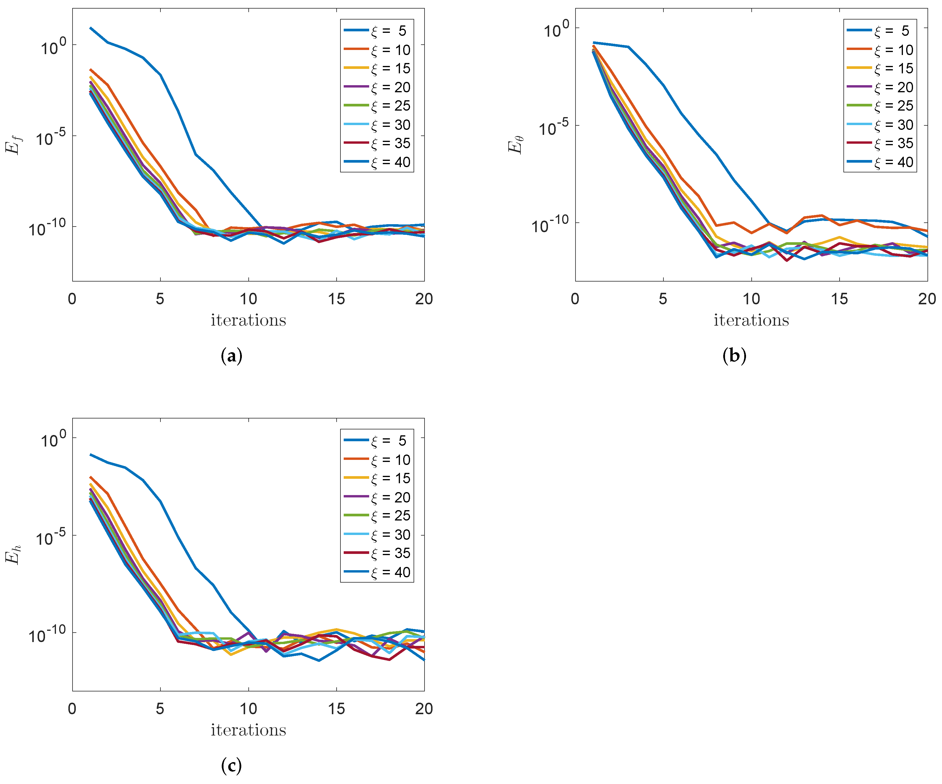
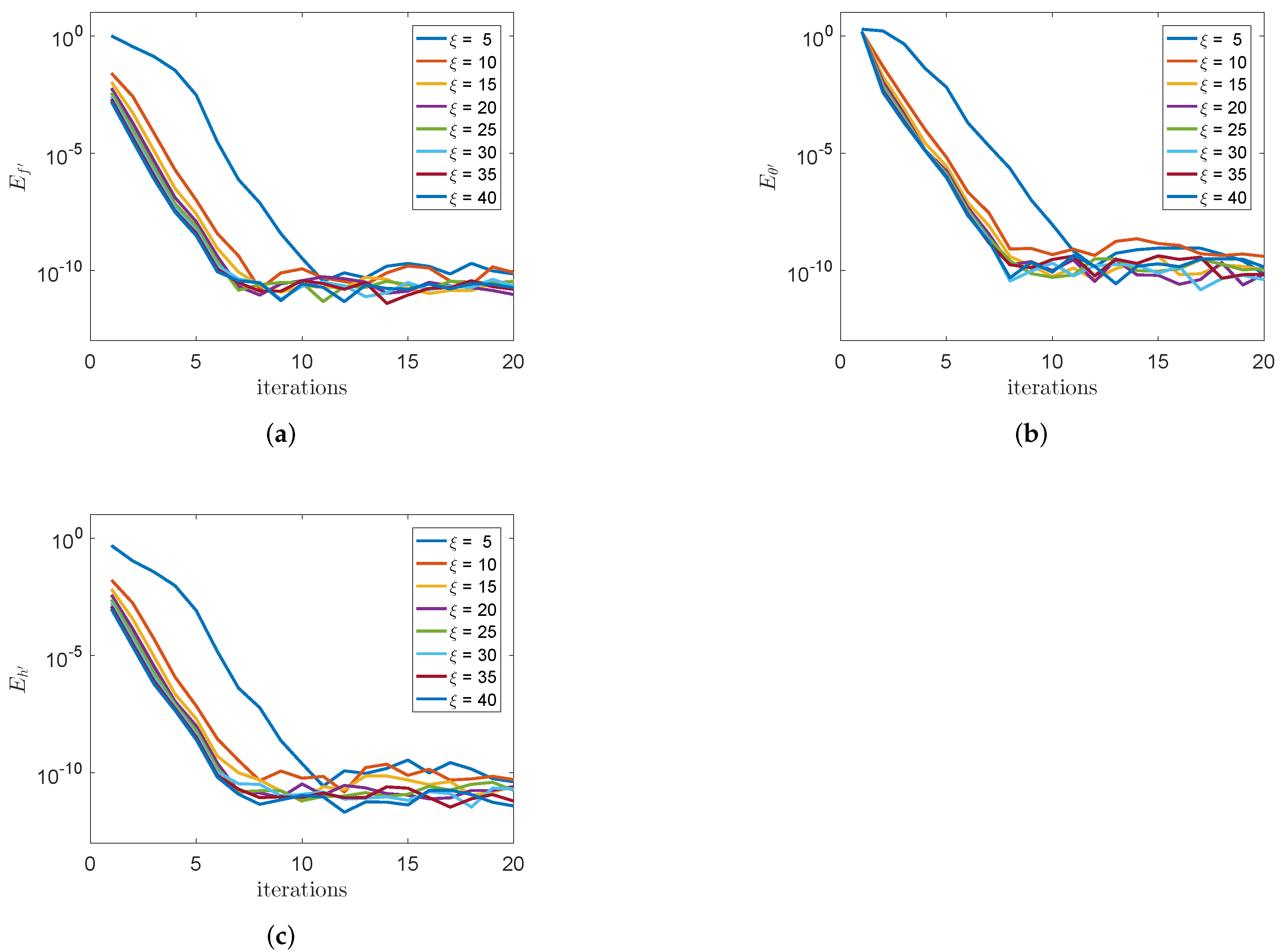
5. Convergence Analysis

The convergence of the MD-BSQLM is discussed in this section. The convergence rate is determined using the infinity norm of the error given by:

$$\mid \mid Q_{s+1}{\left|\right|}_{\infty }=\underset{0\le \epsilon \le N_x}{max}|Q_{s+1}-Q_s|\mathrm{for}Q=(f,\theta ,h).$$

(28)

The differences between the approximate values of the functions at the current and previous iterations are depicted in Figure 2 and Figure 3. The convergence of the method is achieved by the sixth iteration for both the functions and their derivatives. The graphs show that the MD-BSQLM converges rapidly with a high degree of accuracy. The method may be extended to solve other types of highly non-linear differential equations.

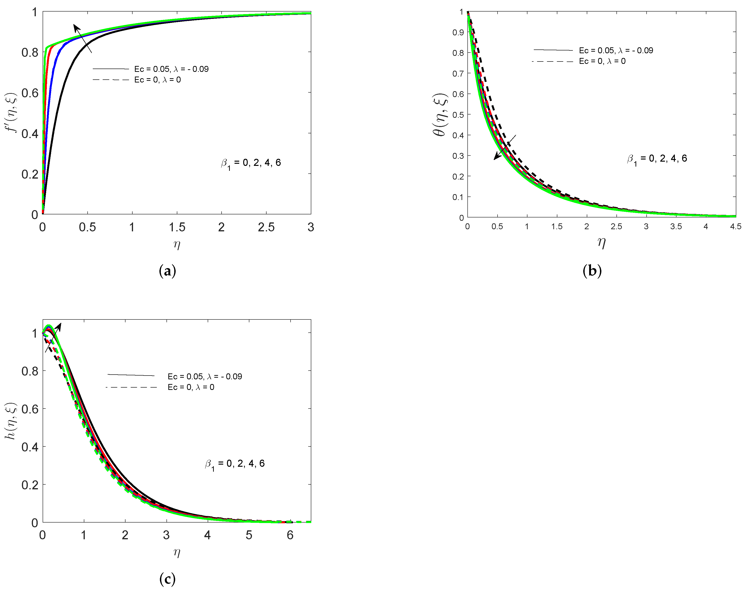
6. Results and Discussion

In this section, we present tabulated results and graphical representations of different features of the fluid flow and heat and mass transfer under the effects of several parameters. The quantities of engineering interest, such as skin fraction and Nusselt and Sherwood numbers are computed and presented in

Table 1. Skin friction, and heat and mass transfer coefficients for ${\beta }_1=0.5,G{r}_T=G{r}_C=0.5,\lambda =-0.09,Ec=0.05,Le=0.4$, and $R_1=0.3$.

$\mathit{\xi }$	Nt	Nb	Nr	Pr	Cfx	Nux	Shx
5					3.0874257	−1.5088474	0.4653439
10	0.001	0.001	0.5	6.8	4.3131008	−1.9976737	0.9329592
15					5.2604334	−2.3949035	1.3198495
20					6.0620646	−2.7411796	1.6592534
	0.001				5.187825	2.154772	−0.008580
10	0.3	0.001	0.5	6.8	5.488176	1.989699	−3.770309
	0.5				5.656798	1.881303	−5.678613
	0.7				5.803213	1.776072	−7.140323
		0.001			6.003369	2.503334	−0.068861
15	0.001	0.1	0.5	6.8	5.992718	2.466485	−0.033776
		0.15			5.988566	2.520528	−0.027644
		0.2			5.970386	3.233199	−0.013723
			0.001		5.198892	2.432598	−0.011509
10	0.001	0.001	0.1	6.8	5.196294	2.362772	−0.010779
			0.2		5.193907	2.301212	−0.010132
			0.3		5.191718	2.246864	−0.009559

. The fluid flow equations were solved numerically using the multi-domain bivariate spectral quasi-linearization method for the chosen parameter values.

A comparison with previously computed results is depicted in

Table 2. Comparison of the values of $-{\theta }^{\prime }(0,0)$ for different values of $Pr$.

Pr	Chamkha et al. [19]	Yih [31]	Present Results
	Finite-Difference Method	Keller Box Method	MD-BSQLM
$0.1$	$0.142003$	$0.140034$	$0.1400343$
$1.0$	$0.332173$	$0.332057$	$0.3320571$
$10.0$	$0.728310$	$0.728141$	$0.7281412$
$100.0$	$1.572180$	$1.571831$	$1.5718323$
$1000.0$	$3.388090$	$3.387083$	$3.3870854$
$10,000.0$	$7.300800$	$7.297402$	$7.2974001$

. These results are comparable to those of Chamkha et al. [19] and Yih [31], which show that this method is robust and gives accurate results.

Figure 4a,c show increases in velocity and concentration with higher values of the variable viscosity parameter (${\beta }_1$). This is true from the Poiseuille law, as the pressure and viscosity within the flow region increase, leading to the observed increase in both flow rate and concentration. The fluid temperature reduces, as most of the thermal energy is lost through convection and conduction to the walls of the sheet, as depicted in Figure 4b.

Table 1 gives the computed skin friction and heat and mass transfer coefficients for different values of the selected parameters. It is noted that the coefficient of skin friction increases for higher values of the non-dimensional number ($\xi$), thermal radiation ($Nr$), and thermophoresis parameters ($Nt$). The dynamic pressure on the surface of the sheet is increased due to the force generated by an increased temperature gradient. The heat transfer coefficient was observed to decrease with higher values of $Nr$ and $Nt$ and increase with $\xi$. The exponentially stretching sheet of the vibrating sheet emits thermal energy through conduction of the fluid particles, which causes the Nusselt number to decrease. The Sherwood number increases with higher values of $\xi$ and $Nt$ and decreases with an increase in the Brownian motion ($Nb$) or any thermophoresis parameter. The force generated by the increased temperature gradient in the fluid causes an increase in mass energy transfer through convection at the vibrating sheets, resulting in a higher mass transfer coefficient. Similar results were obtained by [32,33].

Higher emitted thermal radiation increases the boundary layer temperature, as clearly depicted in Figure 5a. Heat energy in the form of electromagnetic radiation is emitted by the vibrating sheets and transferred to the fluid, causing the temperature to increase. The concentration profiles decrease with higher values of $Nr$, as displayed in Figure 5b.

The Soret effect is observed in Figure 6a–c. Higher values of the thermophoresis parameter lead to increases in all three flow profiles. This can be explained by the fact that the exponentially stretching sheet causes an upward shift in the temperature gradient. The movement of fluid particles in the hot region and high energy levels displace the fluid particles in the cold region, making the three flow variables increase. Similar results were obtained by [34].

The impacts of the local Reynolds ($Re$) and Brinkman numbers ($Br$) on entropy generation are displayed in Figure 7a,b, respectively. Entropy generation increases with higher values of the Reynolds number. The force due to the momentum of the fluid flow causes the inertial forces to increase, and as a result, the irreversibility associated with the flow increases. A similar trend can be observed for the Brinkman number. With higher values of $Br$, more thermal energy is produced by viscous dissipation than thermal energy produced by molecular dissipation. This will thus mean slower heat conduction, and the temperature rises, causing more entropy generation.

The influences of the temperature difference parameter ($\Omega$) and the temperature Grashof number ($G{r}_T$) on entropy generation are depicted in Figure 8a,b, respectively. Entropy generation can be observed to reduce with higher values of $\Omega$; the opposite can be observed with increasing values of $G{r}_T$. The rate of entropy generation increases as a result of increased buoyancy force due to spatial variation in the density of the fluid caused by the temperature difference.

7. Conclusions

In this study, the physical influences of certain parameters on nanofluid flow and heat-mass transfer past an exponentially stretching sheet, and entropy generation, have been analyzed. From this study, we may conclude as follows:

• The MD-BSQLM converges rapidly with a high degree of accuracy. The accuracy may be enhanced by increasing the number of collocation points.
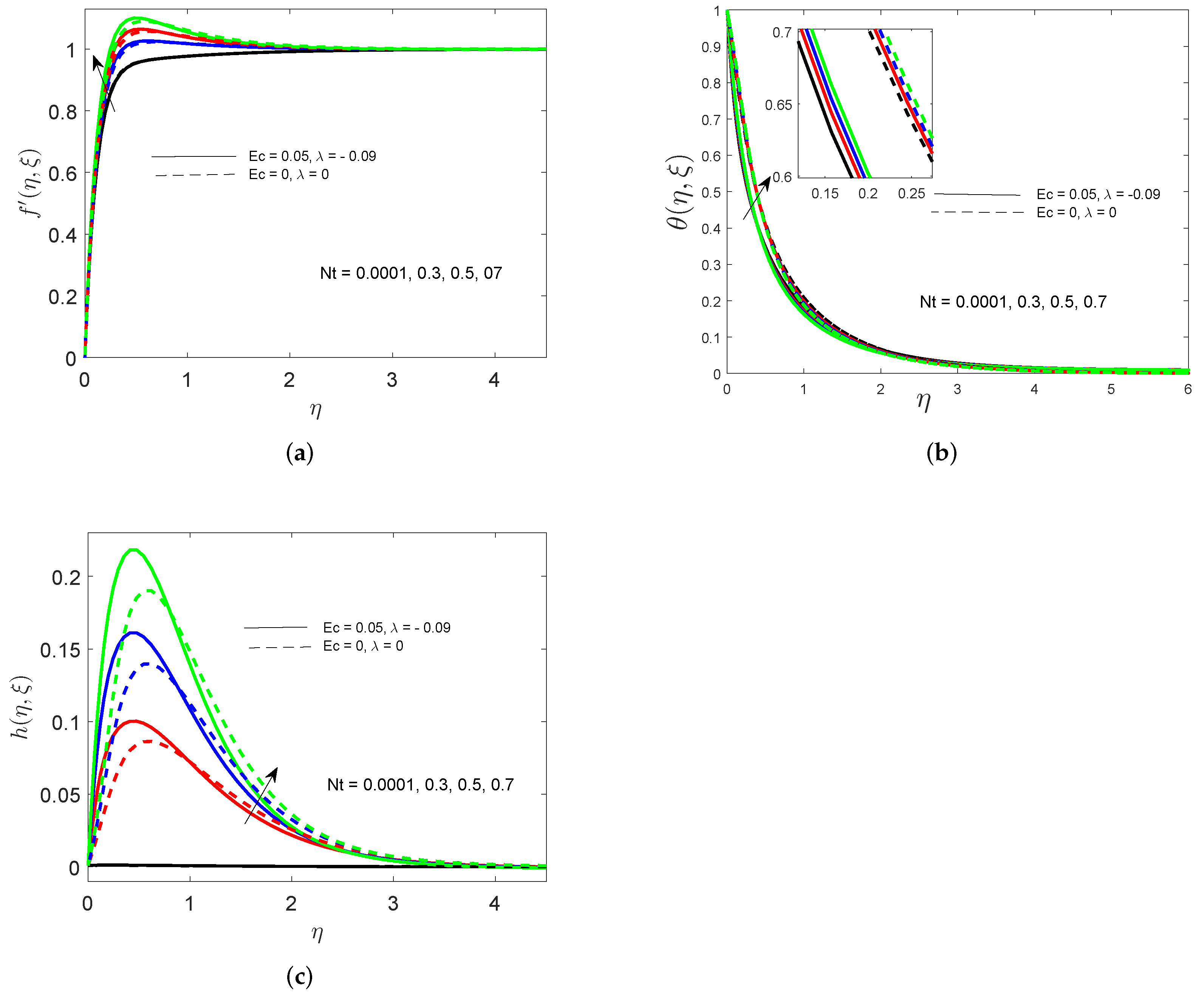
• Increases in thermophoresis and thermal radiation parameters lead to increases in both the skin friction and mass transfer coefficients.
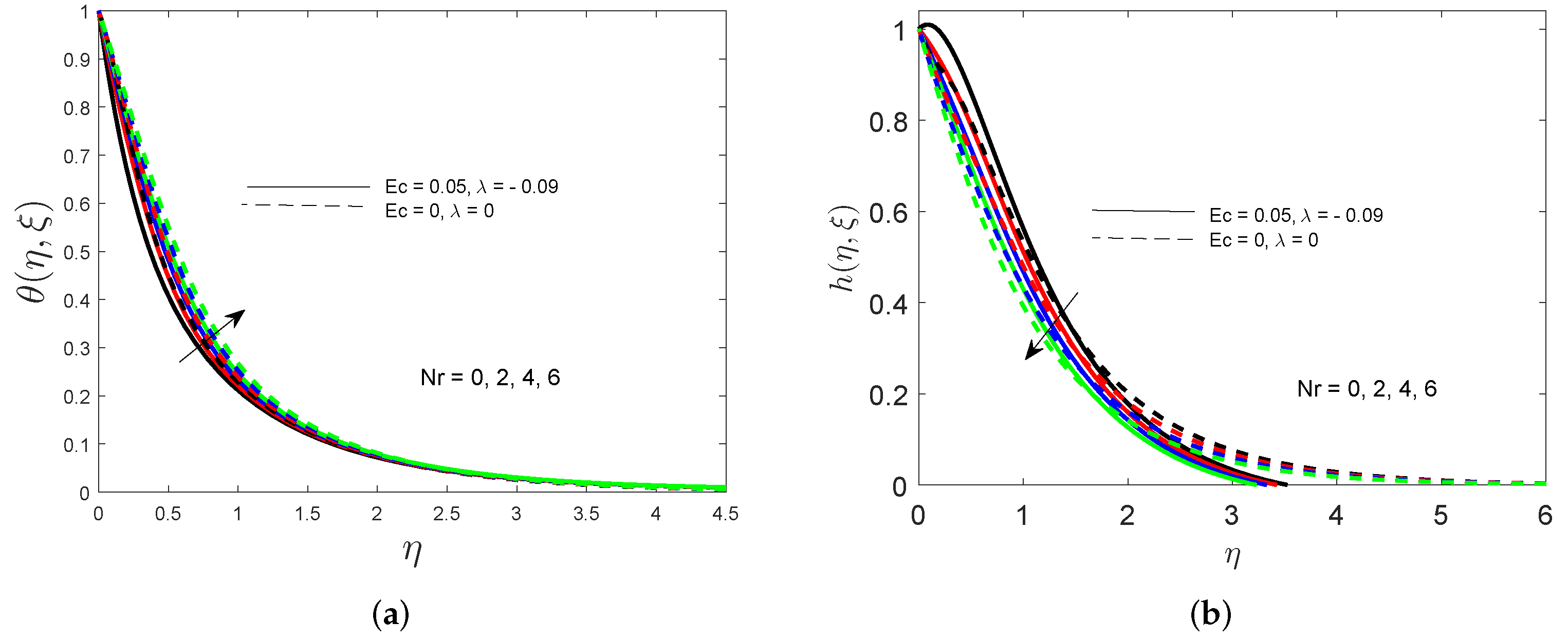
• An increase in thermophoresis, Brownian motion, or thermal radiation parameters leads to a decrease in the rate of heat transfer.
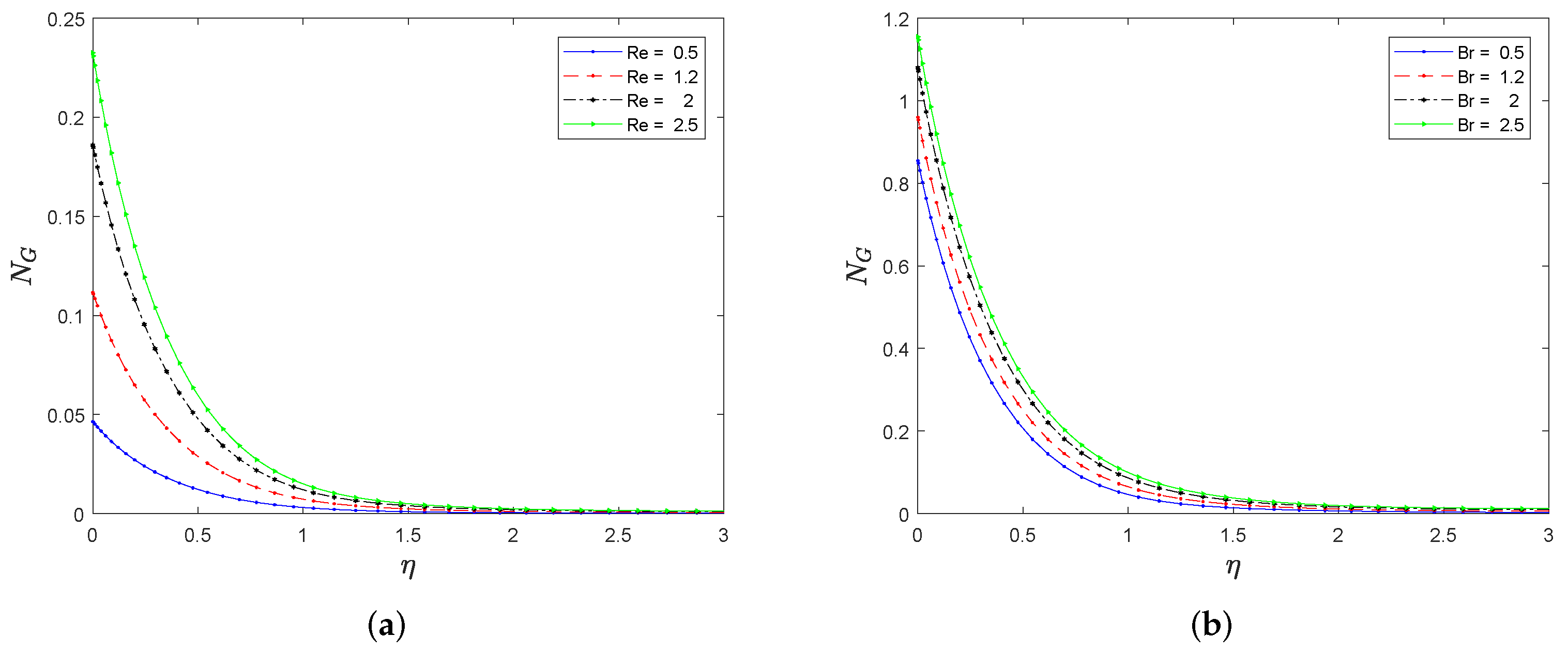
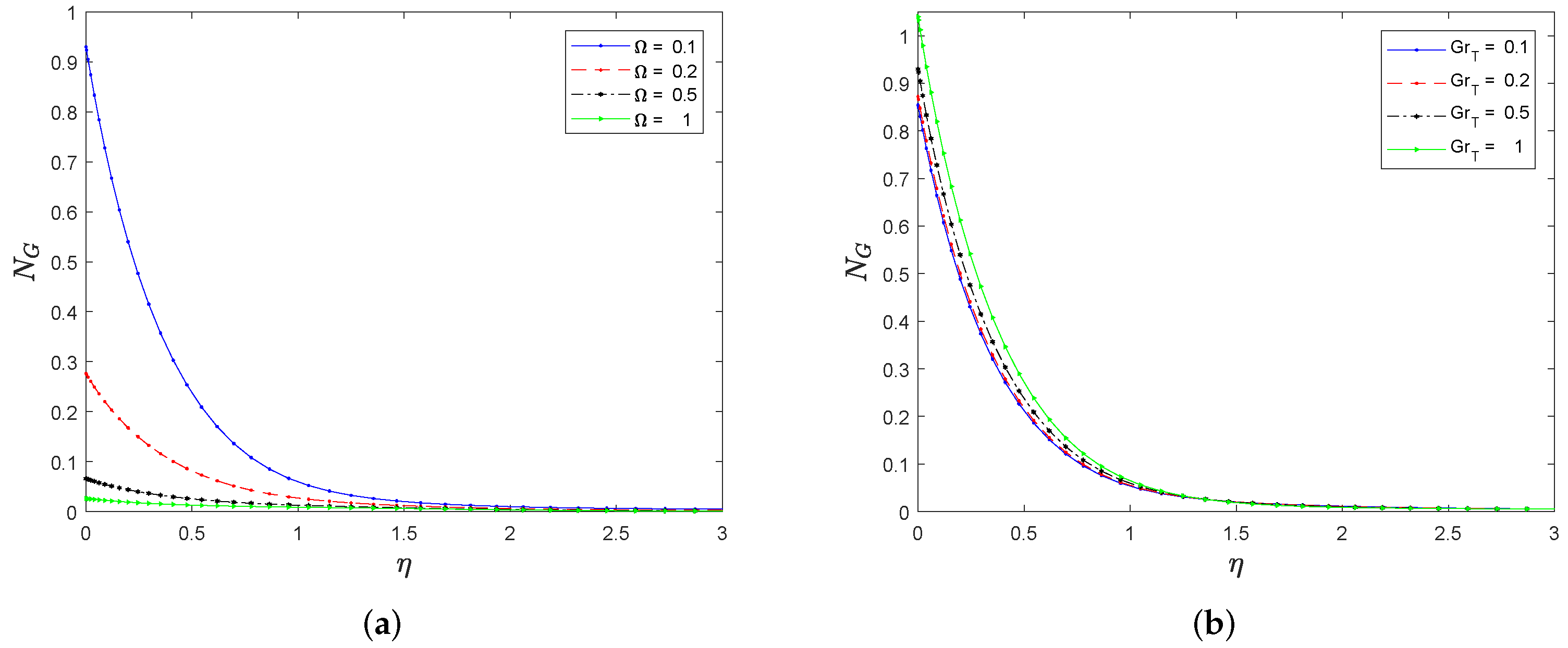
• The entropy generation rate can be minimized through the temperature difference parameter and temperature Grashof number.

References

1. VeeraKrishna, M.; Reddy, M.G. MHD free convective rotating flow of visco-elastic fluid past an infinite vertical oscillating porous plate with chemical reaction. IOP Conf. Ser. Mater. Sci. Eng. 2016, 149, 012217. [Google Scholar]
2. Kataria, H.R.; Patel, H.R. Soret and heat generation effects on MHD Casson fluid flow past an oscillating vertical plate embedded through porous medium. Alex. Eng. J. 2016, 55, 2125–2137. [Google Scholar] [CrossRef] [Green Version]
3. Nadeem, S.; Lee, C. Boundary layer flow of nanofluid over an exponentially stretching surface. Nanoscale Res. Lett. 2012, 7, 1–6. [Google Scholar] [CrossRef] [PubMed] [Green Version]
4. Haq, R.U.; Nadeem, S.; Khan, Z.H.; Okedayo, T.G. Convective heat transfer and MHD effects on Casson nanofluid flow over a shrinking sheet. Cent. Eur. J. Phys. 2014, 12, 862–871. [Google Scholar] [CrossRef]
5. Rehman, F.U.; Nadeem, S.; Rehman, H.U.; Haq, R.U. Thermophysical analysis for three-dimensional MHD stagnation-point flow of nano-material influenced by an exponential stretching surface. Results Phys. 2018, 8, 316–323. [Google Scholar] [CrossRef]
6. Makinde, O.D.; Aziz, A. Boundary layer flow of a nanofluid past a stretching sheet with a convective boundary condition. Int. J. Therm. Sci. 2011, 50, 1326–1332. [Google Scholar] [CrossRef]
7. Barletta, A.; Celli, M.; Rees, D.A. The onset of convection in a porous layer induced by viscous dissipation: A linear stability analysis. Int. J. Heat Mass Transf. 2009, 52, 337–344. [Google Scholar] [CrossRef]
8. Ramesh, G. Influence of shape factor on hybrid nanomaterial in a cross flow direction with viscous dissipation. Phys. Scr. 2019, 94, 105224. [Google Scholar] [CrossRef]
9. Rehman, K.U.; Shatanawi, W.; Ashraf, S.; Kousar, N. Numerical Analysis of Newtonian Heating Convective Flow by Way of Two Different Surfaces. Appl. Sci. 2022, 12, 2383. [Google Scholar] [CrossRef]
10. Rehman, K.U.; Shatanawi, W.; Abodayeh, K.; Shatnawi, T.A. A Group Theoretic Analysis of Mutual Interactions of Heat and Mass Transfer in a Thermally Slip Semi-Infinite Domain. Appl. Sci. 2022, 12, 2000. [Google Scholar] [CrossRef]
11. Rashidi, M.; Ganesh, N.V.; Hakeem, A.A.; Ganga, B.; Lorenzini, G. Influences of an effective Prandtl number model on nano boundary layer flow of γ Al2O3–H2O and γ Al2O3–C2H6O2 over a vertical stretching sheet. Int. J. Heat Mass Transf. 2016, 98, 616–623. [Google Scholar] [CrossRef]
12. Almakki, M.; Mondal, H.; Kameswaran, P.K.; Sibanda, P. Entropy generation in Casson nanofluid flow over a surface with nonlinear thermal radiation and binary chemical reaction. Heat Transf. 2021, 50, 4855–4870. [Google Scholar] [CrossRef]
13. Almakki, M.; Mondal, H.; Sibanda, P. Entropy generation in MHD flow of viscoelastic nanofluids with homogeneous-heterogeneous reaction, partial slip and nonlinear thermal radiation. J. Therm. Eng. 2020, 6, 327–345. [Google Scholar] [CrossRef] [Green Version]
14. Hosseinzadeh, K.; Asadi, A.; Mogharrebi, A.; Khalesi, J.; Mousavisani, S.; Ganji, D. Entropy generation analysis of (CH2OH) 2 containing CNTs nanofluid flow under effect of MHD and thermal radiation. Case Stud. Therm. Eng. 2019, 14, 100482. [Google Scholar] [CrossRef]
15. Aziz, A.; Jamshed, W.; Aziz, T.; Bahaidarah, H.M.; Rehman, K.U. Entropy analysis of Powell–Eyring hybrid nanofluid including effect of linear thermal radiation and viscous dissipation. J. Therm. Anal. Calorim. 2021, 143, 1331–1343. [Google Scholar] [CrossRef]
16. Pal, D.; Mondal, S.; Mondal, H. Entropy generation on MHD Jeffrey nanofluid over a stretching sheet with nonlinear thermal radiation using spectral quasilinearisation method. Int. J. Ambient. Energy 2021, 42, 1712–1726. [Google Scholar] [CrossRef]
17. Maleki, H.; Safaei, M.R.; Togun, H.; Dahari, M. Heat transfer and fluid flow of pseudo-plastic nanofluid over a moving permeable plate with viscous dissipation and heat absorption/generation. J. Therm. Anal. Calorim. 2019, 135, 1643–1654. [Google Scholar] [CrossRef]
18. Sharma, K.; Gupta, S. Viscous dissipation and thermal radiation effects in MHD flow of Jeffrey nanofluid through impermeable surface with heat generation/absorption. Nonlinear Eng. 2017, 6, 153–166. [Google Scholar] [CrossRef]
19. Chamkha, A.J.; Mujtaba, M.; Quadri, A.; Issa, C. Thermal radiation effects on MHD forced convection flow adjacent to a non-isothermal wedge in the presence of a heat source or sink. Heat Mass Transf. 2003, 39, 305–312. [Google Scholar] [CrossRef]
20. Pal, D.; Mondal, H. Influence of temperature-dependent viscosity and thermal radiation on MHD forced convection over a non-isothermal wedge. Appl. Math. Comput. 2009, 212, 194–208. [Google Scholar] [CrossRef]
21. Almakki, M.; Mondal, H.; Sibanda, P. Onset of unsteady MHD micropolar nanofluid flow with entropy generation. Int. J. Ambient. Energy 2021, 1–14. [Google Scholar] [CrossRef]
22. Bejan, A. Entropy generation minimization: The new thermodynamics of finite-size devices and finite-time processes. J. Appl. Phys. 1996, 79, 1191–1218. [Google Scholar] [CrossRef] [Green Version]
23. Rashidi, M.; Mohammadi, F.; Abbasbandy, S.; Alhuthali, M. Entropy Generation Analysis for Stagnation Point Flow in a Porous Medium over a Permeable Stretching Surface. J. Appl. Fluid Mech. 2015, 8. [Google Scholar] [CrossRef]
24. Motsa, S.; Dlamini, P.; Khumalo, M. A new multistage spectral relaxation method for solving chaotic initial value systems. Nonlinear Dyn. 2013, 72, 265–283. [Google Scholar] [CrossRef]
25. Oyelakin, I.; Mondal, S.; Sibanda, P. A multi-domain spectral method for non-Darcian mixed convection flow in a power-law fluid with viscous dissipation. Phys. Chem. Liq. 2018, 56, 771–789. [Google Scholar] [CrossRef]
26. Mondal, S.; Sibanda, P.; Oyelakin, I.S. A multi-domain bivariate approach for mixed convection in a Casson nanofluid with heat generation. Walailak J. Sci. Technol. (WJST) 2018, 16, 681–699. [Google Scholar]
27. Bellman, R.E.; Kalaba, R.E. Quasilinearization and Nonlinear Boundary-Value Problems; Rand Corporation: Santa Monica, CA, USA, 1965. [Google Scholar]
28. Motsa, S.S.; Dlamini, P.G.; Khumalo, M. Spectral relaxation method and spectral quasilinearization method for solving unsteady boundary layer flow problems. Adv. Math. Phys. 2014, 2014, 341964. [Google Scholar] [CrossRef]
29. Motsa, S.S.; Awad, F.G.; Makukula, Z.G.; Sibanda, P. The spectral homotopy analysis method extended to systems of partial differential equations. Abstr. Appl. Anal. 2014, 2014, 241594. [Google Scholar] [CrossRef] [Green Version]
30. Trefethen, L.N. Spectral Methods in MATLAB; SIAM: Philadelphia, PA, USA, 2000. [Google Scholar]
31. Yih, K. MHD forced convection flow adjacent to a non-isothermal wedge. Int. Commun. Heat Mass Transf. 1999, 26, 819–827. [Google Scholar] [CrossRef]
32. Mburu, Z.; Nayak, M.; Mondal, S.; Sibanda, P. Impact of irreversibility ratio and entropy generation on three-dimensional Oldroyd-B fluid flow with relaxation–retardation viscous dissipation. Indian J. Phys. 2022, 96, 151–167. [Google Scholar] [CrossRef]
33. Mburu, Z.M.; Mondal, S.; Sibanda, P.; Sharma, R.P. The Overlapping Grid Spectral Collocation Method for Solving Entropy Generation in Casson Nanofluid Flow Past a Stretching Plate. J. Nanofluids 2021, 10, 45–57. [Google Scholar] [CrossRef]
34. Mburu, Z.M.; Mondal, S.; Sibanda, P. Numerical study on combined thermal radiation and magnetic field effects on entropy generation in unsteady fluid flow past an inclined cylinder. J. Comput. Des. Eng. 2021, 8, 149–169. [Google Scholar] [CrossRef]
Figure 1. The flow schematic diagram.
Applsci 12 10809 g001
Figure 2. Error in (a) f ( η , ξ ) (b) θ ( η , ξ ) , and (c) h ( η , ξ ) for different values of ξ .
Applsci 12 10809 g002
Figure 3. Error in (a) f ( η , ξ ) (b) θ ( η , ξ ) , and (c) h ( η , ξ ) for different values of ξ .
Applsci 12 10809 g003
Figure 4. (a) Velocity; (b) temperature, and (c) concentration profiles for different values of the viscosity parameter.
Applsci 12 10809 g004
Figure 5. The impacts of thermal radiation on (a) temperature and (b) concentration profiles.
Applsci 12 10809 g005
Figure 6. Impacts of the thermophoresis parameter on (a) velocity, (b) temperature, and (c) concentration profiles.
Applsci 12 10809 g006
Figure 7. The influences of (a) the local Reynolds and (b) Brinkman numbers on the entropy generation profiles.
Applsci 12 10809 g007
Figure 8. The influences of (a) the temperature difference parameter, and (b) temperature Grashof number on the entropy generation profiles.
Applsci 12 10809 g008