Modelling and Analysis of Viscoelastic and Nanofluid Effects on the Heat Transfer Characteristics in a Double-Pipe Counter-Flow Heat Exchanger

Abstract

This study computationally investigates the heat transfer characteristics in a double-pipe counter-flow heat-exchanger. A heated viscoelastic fluid occupies the inner core region, and the outer annulus is filled with a colder Newtonian-Fluid-Based Nanofluid (NFBN). A mathematical model is developed to study the conjugate heat transfer characteristics and heat exchange properties from the hot viscoelastic fluid to the colder NFBN. The mathematical modelling and formulation of the given problem comprises of a system of coupled nonlinear partial differential Equations (PDEs) governing the flow, heat transfer, and stress characteristics. The viscoelastic stress behaviour of the core fluid is modelled via the Giesekus constitutive equations. The mathematical complexity arising from the coupled system of transient and nonlinear PDEs makes them analytically intractable, and hence, a recourse to numerical and computational methodologies is unavoidable. A numerical methodology based on the finite volume methods (FVM) is employed. The FVM algorithms are computationally implemented on the OpenFOAM software platform. The dependence of the field variables, namely the velocity, temperature, pressure, and polymeric stresses on the embedded flow parameters, are explored in detail. In particular, the results illustrate that an increase in the nanoparticle volume-fraction, in the NFBN, leads to enhanced heat-exchange characteristics from the hot core fluid to the colder shell NFBN. Specifically, the results illustrate that the use of NFBN as the coolant fluid leads to enhanced cooling of the hot core-fluid as compared to using an ordinary (nanoparticle free) Newtonian coolant.

1. Introduction

The development of efficient heat-transfer-fluids (HTF) continues to attract the attention of scientists and engineers given the widespread applications. The development and enhancement of efficient HTF has been widely investigated experimentally, theoretically, and computationally, see for example [1,2,3,4,5,6,7,8,9,10,11,12,13,14]. Such widespread investigations have been conducted with a view to the important industrial applications of HTF, say, to polymer processing, food and beverage processing, chemical processing, pharmaceutical manufacture, etc.

The concept and development of nanofluids has largely arisen as a route to heat-transfer-rate (HTR) enhancement and efficient performance of HTF. Nanofluids are a dispersion of solid (metallic) nanometer-sized particles (nanoparticles) in a base-fluid. The available literature, see for example [9,15,16,17,18], has shown that nanofluids exhibit higher thermal conductivities as compared to the conventional (and corresponding) base-fluids. The literature specifically demonstrates that such higher thermal conductivities of nanofluids lead to increases in heat-transfer-rates (HTR) as compared to the corresponding base-fluids. Additionally, ongoing research has demonstrated that the attractive heat-transfer characteristics of nanofluids can be further improved via various methods including increasing the Brownian motion of the embedded nanoparticles suspended in the base-fluids [19,20,21], increasing volume-fraction of the embedded nanoparticles [22,23,24], increasing the fluid layers around the embedded nanoparticles [19,20], etc. The present research specifically explores the effects, on HTR enhancement, of nanoparticle volume-fraction (i.e., concentration of nanoparticles) in the nanofluid.

In comparative investigations on the thermal conductivities of nanofluids versus the corresponding base-fluids, [25] reported that up to $30\%$ increase in the thermal conductivity can be observed in nanofluids generated from various nanoparticle/base-fluid combinations, e.g., ${\mathit{Al}}_2{O}_3$-water, ${\mathit{SiO}}_2$-water, and ${\mathit{TiO}}_2$-water. Similar results were also reported in [1] using $\mathit{CuO}$-water, ${\mathit{Al}}_2{O}_3$-water, and $\mathit{Co}$-oil nanofluids. The authors in [26] claimed a $100\%$ increase in thermal conductivity for a range of volume-fractions 0.5–10% of aluminium particles in a water base. The results of [27] showed that a $\mathit{Cu}$-ethylene glycol nanofluid with a volume fraction of $0.3\%$ produced a $40\%$ increase in thermal conductivity. The investigation in [8] reported up to $78\%$ rise in thermal conductivity for $\mathit{Cu}$-water nanofluids at a $75\%$ volume fraction of nanoparticles.

Akin to thermal conductivity enhancements investigations, studies have also been conducted on the effect of nanofluids on convective heat-transfer. The authors in [28], for example, investigated the performance of a nanofluid containing carbon nanotubes and observed that the convective heat-transfer rate can be as much as $3.5$ times higher than that of the corresponding water base. Similarly, the authors in [29], using an ${\mathit{Al}}_2{O}_3$-water nanofluid, reported a convective heat-transfer rate rise of $40\%$. The investigations in [30,31], on the convective heat-transfer coefficient of deionised water with a dispersion of $Cu$ nanoparticles for both laminar and turbulent flows in a tube, demonstrated higher convective heat-transfer coefficients for the nanofluids than for the deionised water base.

Even though nanofluids may physically never be truly homogeneous mixtures, the mathematical modelling of nanofluids is nonetheless generally divided into the two classes, namely single-phase (homogeneous) and two-phase (heterogeneous), see for example [32,33,34]. In the single-phase model, which is adopted in the present work, the nanofluid is treated as a homogeneous fluid mixture and the conventional fluid dynamical governing equations are modified to incorporate the volume-fractions of the embedded nanoparticles, see for example [32,33]. In the two-phase model, the base-fluid phase has its own fluid-dynamical governing equations, and a concentration equation is required to account for the effects of the suspended nanoparticles, see for example [34]. Empirical investigations for the two-phase models have demonstrated that for nanofluids with low nanoparticle volume fractions, the Lagrangian–Eulerian formulation is preferred, see for example [35], in which this approach was employed in analysing the HTR effects of $Cu$ and ${\mathit{Al}}_2{O}_3$ nanoparticles under turbulent flow conditions. For the reverse scenario of nanofluids with high nanoparticle volume fractions, the more suitable approach would be the Eulerian–Eulerian formulation, see for example [36], who conducted numerical simulations for laminar forced convection heat-transfer of $Cu$-water nanofluids in isothermally heated microchannels.

In addition to the above motivations and literature on HTF, with regards to industrial heating and cooling applications, the present study is additionally spurred on by the investigations in [32,33]. The investigations in [32,33] specifically explored the non-isothermal effects of various viscoelastic-fluid-based nanofluids. Additional motivation arises from the works in [37,38], which investigated the heat exchanger dynamics using particle-free viscoelastic and Newtonian fluids. The present investigation is aimed at the need to add to the literature on the development, design, and performance of industrial heat exchangers with a focus on the use and effects of nanofluids. The current work may also be extended to heat-exchange problems involving phase change and boiling, in which case the important surface-tension effects would need to be accounted for, including the effects to the energy conservation, see [39].

The present work employs finite volume computational methodologies implemented on the open-source OpenFOAM software platform [38,40,41,42]. The OpenFOAM software platform offers the flexibility and convenience to incorporate new computational fluid dynamics (CFD) models via modifications of already-existing solvers, see for example [43,44,45,46,47]. The additional purpose of this work is therefore the development of a solver, under the OpenFOAM framework, for heat exchange investigations involving viscoelastic fluids and Newtonian-Fluid-Based Nanofluids (NFBN).

The paper is structured as follows. In Section 2, the mathematical model formulation is presented. The development of numerical algorithms is given in Section 3. In Section 4, graphical computational results and discussion of results are presented. Finally, the concluding remarks are given in Section 5.

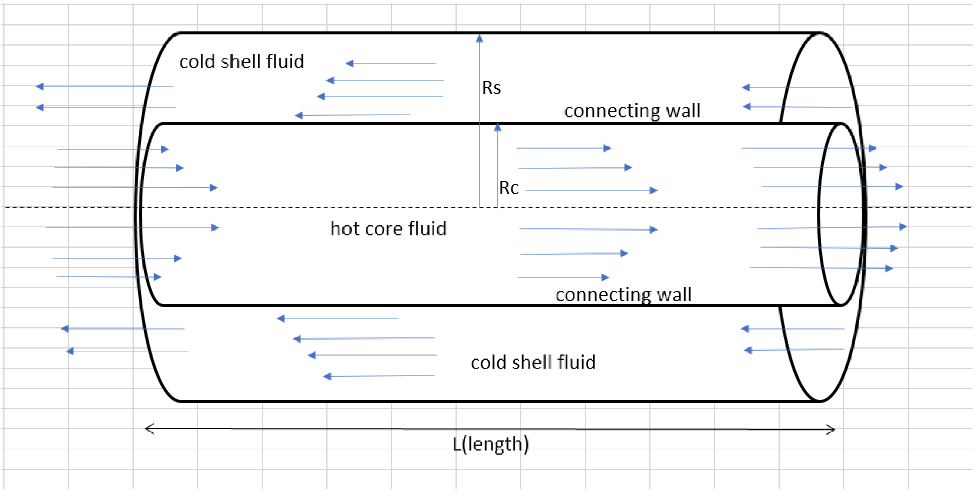
2. Mathematical Model

Two hollow concentric cylindrical pipes are arranged in a double-pipe geometry with an inner cylinder (the core) located inside an outer cylinder (the shell), see Figure 1. Both cylinders are of equal length, L, in the longitudinal direction, i.e., the z-direction.

The inner (core) cylinder has a radius $R_c$ in the radial direction, i.e., the r-direction, and is symmetrically surrounded by an outer cylinder (the shell) of radius $R_s$, with $0<R_c<R_s$. The cylindrical coordinate system $(r,\theta ,z)$ is adopted, with r in the radial direction, $\theta$ in the angular direction, and z in the longitudinal direction.

Axi-symmetric conditions are assumed, and hence, all flow field variables will be considered independent of $\theta$. For example, the velocity field would therefore be of the form $\mathit{V}=\left(u\right(r,z),0,w(r,z\left)\right)$, where u is the velocity component in the radial (r) direction and w is the velocity component in the longitudinal (z) direction.

Laminar, incompressible, time-dependent, and non-isothermal conditions are additionally assumed. A heated/hot viscoelastic fluid occupies the inner core region and flows, say in the positive z-direction. A colder NFBN fills the outer annulus and flows in the opposite direction to the core fluid leading to the counter-flow arrangement.

2.1. Governing Equations for Core-Fluid

In dimensional terms, the governing mathematical equations for the viscoelastic core-fluid are derived from the conservation of mass, momentum, and energy, respectively, detailed in Equations (1)–(3):

$${\nabla }^{*}·{\mathit{U}}_c^{*}=0,$$

(1)

$${\rho }_c^{*}\left(\frac{\partial {\mathit{U}}_c^{*}}{\partial t^{*}}+{\mathit{U}}_c^{*}·{\nabla }^{*}{\mathit{U}}_c^{*}\right)=-{\nabla }^{*}{p}_c^{*}+{\nabla }^{*}·{\mathbf{\sigma }}_c^{*}+{\mathit{F}}_c^{*},$$

(2)

$${\rho }_c^{*}{C}_{p_c}^{*}\left(\frac{\partial T_c^{*}}{\partial t^{*}}+T_c^{*}·{\nabla }^{*}{T}_c^{*}\right)=Q_{D_c}^{*}-{\nabla }^{*}·{\Phi }_{q_c}+h_c^{*}(T_w^{*}-T_c^{*}).$$

(3)

The asterisks ∗ in Equations (1)–(3) represent dimensional variables, the subscript ${\left(\right)}_c$ denotes core-fluid, ${\nabla }^{*}$ is the gradient operator, ${\mathit{U}}_c^{*}$ is the velocity field, ${\rho }_c^{*}$ the density, $t^{*}$ the time, $p_c^{*}$ the pressure field, ${\mathbf{\sigma }}_c^{*}$ the total stress tensor, ${\mathit{F}}_c^{*}$ represents body forces, $C_{p_c}^{*}$ is the specific heat at constant pressure, $T_c^{*}$ is the temperature field of the core fluid, $Q_{D_c}^{*}$ the internal heat production, ${\Phi }_{q_c}^{*}$ the heat flux vector, $T_w^{*}$ is the connecting wall temperature, and $h_c^{*}$ and $h_s^{*}$ are a convective heat-transfer parameters.

The total stress tensor is given by:

$${\mathbf{\sigma }}_c^{*}=-{p_c}^{*}{\mathit{I}}^{*}+{\mathbf{\tau }}_c^{*}+{\eta }_c^{*}{\mathit{S}}_c^{*},$$

where $\mathit{I}$ is the identity tensor, ${\mathbf{\tau }}_c^{*}$ represents the polymer-stress tensor, and

$${\mathit{S}}_c^{*}=\left[{\nabla }^{*}{\mathit{U}}_c^{*}+{\left({\nabla }^{*}{\mathit{U}}_c^{*}\right)}^T\right],$$

is the rate of deformation tensor. The internal heat production is expressed as:

$$Q_{D_c}^{*}=\gamma {\mathbf{\tau }}^{*}:{\mathit{S}}_c^{*}+(1-\gamma ){\eta }_{sol}^{*}{\mathit{S}}_c^{*}:{\mathit{S}}_c^{*},$$

where ${\eta }_{sol}^{*}$ is the solvent viscosity and $\gamma$ is a viscoelastic non-isothermal parameter; for the full details, we refer the reader to [47,48,49]. The heat flux is mathematically expressed by Fourier’s law:

$${\Phi }_{q_c}^{*}=-K_c^{*}{\nabla }^{*}{T}_c^{*},$$

where $K_c^{*}$ is the thermal conductivity. The Giesekus viscoelastic constitutive equations are employed to model the polymeric stresses:

$${\mathbf{\tau }}^{*}+{\epsilon }^{*}{{\mathbf{\tau }}^{*}}^2+{\lambda }^{*}\stackrel{\nabla }{{\mathbf{\tau }}^{*}}={\eta }_p^{*}{\mathit{S}}_c^{*},$$

where ${\epsilon }^{*}$ is the Giesekus nonlinear parameter, ${\lambda }^{*}$ is the relaxation time, ${\eta }_p^{*}$ is the polymer viscosity, and $\stackrel{\nabla }{{\mathbf{\tau }}^{*}}$ is the upper convected time derivative defined as:

$$\stackrel{\nabla }{{\mathbf{\tau }}^{*}}=\frac{\partial {\mathbf{\tau }}^{*}}{\partial t^{*}}+({\mathit{U}}_c^{*}·{\nabla }^{*}){\mathbf{\tau }}^{*}-\left({\nabla }^{*}{\mathit{U}}_c^{*}\right){\mathbf{\tau }}^{*}-{\mathbf{\tau }}^{*}{\left({\nabla }^{*}{\mathit{U}}_c^{*}\right)}^T.$$

The relaxation time and viscosity are assumed constant with the total viscosity given by:

$${\eta }_c^{*}={\eta }_{sol}^{*}+{\eta }_p^{*}.$$

2.2. Governing Equations for Shell-Fluid

A Newtonian-Fluid-Based Nanofluid (NFBN) is assumed for the shell-fluid flowing in the outer annulus. The subscript ${\left(\right)}_{sf}$, in the flow variables, is used to denote shell-fluid and the subscript ${\left(\right)}_{nf}$ represents nanofluid. The governing equations for the shell-fluid flow are otherwise similar to those for the core-fluid system, but without the polymer-stress contributions. The equations, in a dimensional form, read:

$${\nabla }^{*}·{\mathit{U}}_{sf}^{*}=0,$$

(4)

$${\left({\rho }_{sf}\right)}_{nf}^{*}\left(\frac{\partial {\mathit{U}}_{sf}^{*}}{\partial t^{*}}+{\mathit{U}}_{sf}^{*}·{\nabla }^{*}{\mathit{U}}_{sf}^{*}\right)=-{\nabla }^{*}{p}_{sf}^{*}+{\nabla }^{*}·{\mathbf{\sigma }}_{sf}^{*},$$

(5)

$${\left({\rho }_{sf}{C}_{p_{sf}}\right)}_{nf}^{*}\left(\frac{\partial T_s^{*}}{\partial t^{*}}+T_{sf}^{*}·{\nabla }^{*}{T}_{sf}^{*}\right)=Q_{D_{sf}}^{*}-{\nabla }^{*}·{\Phi }_{q_{sf}}.$$

(6)

where ${\left({\rho }_{sf}\right)}_{nf}^{*}$ is the NFBN density, ${\sigma }_{sf}^{*}$ the total stress tensor, ${\left({\rho }_{sf}{C}_{p_{sf}}^{*}\right)}_{nf}^{*}$ the NFBN specific heat capacity, $Q_{D_{sf}}^{*}$ the internal heat production, and ${\Phi }_{q_{sf}}^{*}$ the heat-flux vector. The total stress tensor for the shell-fluid is defined as:

$${\mathbf{\sigma }}_{sf}^{*}=\frac{{\eta }_{sol}^{*}}{\sqrt{{(1-\phi )}^5}}{\mathit{S}}_{sf}^{*},$$

where $\phi$ is the nanoparticle volume-fraction. The internal heat production is defined as:

$$Q_{D_{sf}}^{*}=\frac{{\eta }_{sol}^{*}}{\sqrt{{(1-\phi )}^5}}{\mathit{S}}_{sf}^{*}:{\nabla }^{*}{\mathit{U}}_{sf}^{*}.$$

The heat-flux vector follows Fourier’s law:

$${\Phi }_{q_{sf}}^{*}=-K_{nf}^{*}{\nabla }^{*}{T}_{sf}^{*},$$

where $K_{nf}^{*}$ is the nanofluid thermal conductivity, which is defined as:

$$K_{nf}^{*}=\frac{K_s^{*}+(1-\aleph )K_f^{*}+(1-\aleph )\phi (K_f^{*}-K_s)}{K_s^{*}+(1-\aleph )K_f^{*}+\phi (K_f^{*}-K_s^{*})}(1+\alpha A_2{T}_s^{*}),$$

where $A_2$ is a thermal-conductivity parameter and ℵ is an empirical shape-factor. For spherical-shaped nanoparticles, which are assumed in the present work, $\aleph =3$, [50].

The nanofluid quantities, ${\left(\right)}_{nf}$, are obtained from linear combinations of the volume-fractions, $\phi$, of the base-fluid contribution, ${\left(\right)}_f$, and the nanoparticle contribution, ${\left(\right)}_s$. For example:

$$\begin{array}{cc}\hfill {\rho }_{nf}^{*}& =\phi {\left({\rho }_{sf}\right)}_s^{*}+(1-\phi ){\left({\rho }_{sf}\right)}_f^{*},\hfill \\ \hfill & \\ \hfill {\left({\rho }_{sf}{C}_{p_{sf}}\right)}_{nf}^{*}& =\phi {\left({\rho }_{sf}{C}_{p_{sf}}\right)}_s^{*}+(1-\phi )({\left({\rho }_{sf}{C}_{p_{sf}}\right)}_f^{*}.\hfill \end{array}$$

2.3. Governing Equation for the Connecting Wall

The shell-fluid and core-fluid are separated by a connecting wall through which heat-exchange occurs. The governing equation for the connecting wall temperature, $T_w^{*}$, follows the one-dimensional heat conduction equation:

$$\frac{\partial T_w^{*}}{\partial t^{*}}=\frac{{\partial }^2{T}_w^{*}}{\partial {z^{*}}^2}+h_c^{*}(T_c^{*}-T_w^{*})+h_{sf}^{*}(T_{sf}^{*}-T_w^{*}).$$

(7)

3. Numerical Algorithms and Computational Methodologies

Equations (1)–(7) are solved numerically using Finite Volume Methods (FVM). The FVM numerical algorithms are implemented on the OpenFOAM software platform. The OpenFOAM computational solvers that are developed in the present work are adapted and modified from both the viscoelasticFluidFoam and the rheoMultiRegionFoam solvers, which pre-exist on OpenFOAM, see for example [41,42]. These two pre-existing solvers are well adapted to viscoelastic flow simulations, and hence, they are well suited as starting points for the development of the viscoelastic computations required in the present work.

The computational mesh for the double-pipe geometry, Figure 2, is created using the OpenFOAM mesh generation functionality called blockMesh. In OpenFOAM language, this mesh is implemented over a blockMeshDict file, in which the geometry is conveniently defined and results are viewed using the Paraview software.

Viscoelastic flow computations are prone to numerical difficulties which arise at high Weissenberg, $We$, or alternatively at high Deborah, $De$, numbers, leading to the so-called High-Weissenberg-Number-Problem (HWNP). The higher the Weissenberg (or Deborah) number, the more pronounced would be the elastic effects, in which case the viscoelastic fluid largely exhibits solid-like behaviour leading to the numerical instabilities for the fluid-based computations. Both the Discrete-Elastic-Viscous-Stress-Splitting (DEVSS) [42,51] and the Log-Conformation-Reformulation (LCR) techniques [52,53] are employed to mitigate against numerical instabilities arising from the HWNP.

3.1. DEVSS Technique

In the Discrete-Elastic-Viscous-Stress-Splitting (DEVSS) method, employed in the viscoelasticFluidFoam solver, an additional elliptic operator [54] is added on each side of the momentum equations. The stabilising effects of the elliptic terms may be enhanced by scaling them with the polymeric viscosity, ${\eta }_p$, [51,55]. Under the DEVSS technique, the momentum equations take the form:

$$\rho \left(\frac{\partial \mathit{U}}{\partial t}+\mathit{U}·\nabla \mathit{U}\right)-\nabla ·({\eta }_s+{\eta }_p)\nabla \mathit{U}=-\nabla p-\nabla ·({\eta }_p\nabla \mathit{U})+\nabla ·\mathbf{\tau }+\rho \mathit{F}.$$

(8)

3.2. LCR Technique

The Log-Conformation-Reformulation (LCR) approach is implemented for numerical stabilisation in the RheoMultiRegionFoam solver. In the LCR approach, the polymeric-stress tensor, $\mathbf{\tau }$, is replaced with the logarithm of the conformation tensor, $\mathit{D}$, where:

$$\mathbf{\tau }=\frac{{\eta }_p}{\lambda }(\mathit{D}-\mathit{I}).$$

(9)

The process to recast the viscoelastic-stress constitutive-equations in terms of the logarithm of conformation tensor (log-conformation) requires that the stress tensor, $\mathbf{\tau }$, be initially replaced (in the viscoelastic-stress constitutive-equations) by the conformation tensor, $\mathit{D}$, via Equation (9). This initial process leads to the alternative constitutive equations for the conformation tensor:

$$\frac{\partial \mathit{D}}{\partial t}+(\mathit{U}·\nabla )\mathit{D}-(\mathit{D}·\nabla {\mathit{U}}^T+\nabla \mathit{U}·\mathit{D})=-\frac{1}{\lambda }{f}_R\left(\mathit{D}\right),$$

(10)

where $f_R\left(\mathit{D}\right)$ is a polynomial function in the conformation tensor [21]. Since $\mathit{D}$ is positive definite, it can be diagonalised that:

$$\mathit{D}=\mathit{R}·\Lambda ·{\mathit{R}}^T,$$

(11)

where $\mathit{R}$ is an orthogonal matrix containing, as its columns, the eigenvectors of $\mathit{D}$, and $\Lambda$ is a diagonal matrix with corresponding eigenvalues of $\mathit{D}$. The second step in the LCR technique is based on the realisation that it would be more efficient to solve constitutive equation in terms of the logarithm of $\mathit{D}$ (i.e., introduce and solve for, $\Theta =log\mathit{D}$, in the constitutive equations) rather than solving directly for $\mathit{D}$. In particular:

$$\Theta =log\mathit{D}=\mathit{R}·log\Lambda ·{\mathit{R}}^T.$$

(12)

Following [52,53], the velocity gradient, $\nabla \mathit{U}$ can be decomposed as:

$$\nabla \mathit{U}=\Omega +\mathit{B}+\mathit{N}·{\mathit{D}}^{-1},$$

(13)

where both $\Omega$ and $\mathit{N}$ are anti-symmetric and $\mathit{B}$ is a symmetric traceless tensor which commutes with $\mathit{D}$. Equation (10), therefore, reduces to:

$$\frac{\partial \Theta }{\partial t}+(\mathit{U}·\nabla )\Theta -(\Omega \Theta -\Theta \Omega )-2\mathit{B}=\mathit{R}\left[\frac{1}{\lambda }({\Lambda }^{-1}-1)\right]{\mathit{R}}^T.$$

(14)

In a two-dimensional flow, the eigen-decomposition of $\mathit{D}$ can be expressed as:

$$\mathit{D}=\mathit{R}\left[\begin{array}{cc}{\lambda }_1& 0\\ 0& {\lambda }_2\end{array}\right]{\mathit{R}}^T,$$

(15)

where ${\lambda }_1$ and ${\lambda }_2$ are eigenvalues of $\mathit{D}$, and also:

$${\mathit{R}}^T(\nabla \mathit{U})\mathit{R}=\left[\begin{array}{cc}{m}_{11}& 0\\ 0& m_{22}\end{array}\right],\mathit{B}=\mathit{R}\left[\begin{array}{cc}{m}_{11}& 0\\ 0& m_{22}\end{array}\right]{\mathit{R}}^T,\Omega =\mathit{R}\left[\begin{array}{cc}\delta & 0\\ 0& -\delta \end{array}\right]{\mathit{R}}^T,$$

(16)

with:

$$\delta =\frac{(m_{12}+m_{21})}{({\lambda }_2-{\lambda }_1)}.$$

3.3. Pressure Correction

Unlike for compressible flow, where empirical relations such as the ideal gas law allow for a direct/explicit pressure-linked equation, the solution processes for pressure-linked equations for incompressible fluid flow on the other hand are complicated by the reality that there is no explicit pressure equation to solve. Numerical solutions for pressure-linked equations of incompressible fluid flow have led to the development of various techniques to overcome this difficulty. The current investigation employs the Pressure-Implicit-with-Splitting-of-Operators (PISO) algorithm, see for example [56], to deal with this challenge. The PISO algorithm can be summarised as follows.

• Initialise the field variables: velocity $\mathit{U}$, pressure p, polymeric stresses $\mathbf{\tau }$, and temperature T.
• For the LCR approach, solve for the conformation tensor $\mathit{D}$ and $\Theta =log\mathit{D}$.
• For the DEVSS approach, solve directly for the polymer stresses, $\mathbf{\tau }$.
• Solve the momentum equations for the intermediate velocity field, ${\mathit{U}}^{**}$.
• Using the intermediate velocity, $U^{**}$, estimate a new pressure field $p^{**}$. Subsequently, perform a correction of the intermediate velocity field and obtain the new velocity ${\mathit{U}}^{***}$, which must satisfy mass conservation.
• The updated velocity ${\mathit{U}}^{***}$ is then used to compute the polymer-stresses ${\mathbf{\tau }}^{**}$ and temperature $T^{**}$ via the stress constitutive equations and energy equations, respectively.
• Go to step 1 with the field variables $\mathit{U}$, p, $\mathbf{\tau }$, T, respectively, replaced with $U^{***}$, $p^{**}$, ${\tau }^{**}$, and $T^{**}$ and repeat the steps until the required accuracies are achieved or until the required number of iterations is reached.

3.4. Core-Fluid Simulations

3.4.1. Initial and Boundary Conditions in Core Region

The initial conditions are assumed to be zero for all fluid variables except for core temperature, which is initially set to 300 K. At the inlet regions of the pipe sections, the velocities are kept at 2 m/s while pressure is assigned a zero gradient boundary condition. The polymer-stresses are initially fixed at zero throughout the core region. At the outlet, a zero gradient condition is assigned for all fluid variables except for pressure, which is set to zero. The usual no-slip boundary conditions are imposed for velocity at the pipe walls. A zero gradient condition is imposed for polymer-stresses at the pipe walls.

3.4.2. Discretisation Schemes for Core Region

Since the model problem is transient in nature, time discretisation is crucial and must be implemented in a way that enhances numerical stability and convergence. The time derivatives are, therefore, approximated via an implicit Euler scheme. A linear scheme with Gaussian integration is applied on space derivative terms, i.e., the gradient terms. A Gaussian first order upwind scheme is used for the discretisation of the convective terms. The Laplacian terms are discretised via bounded, second-order Gaussian linear corrected schemes.

The systems of linear equations generated by the above space-time discretisations are solved via efficient and robust linear algebraic techniques. Specifically, a Bi-Conjugate Gradient Stabilised (BiCGStab) solver is used for the discretised velocity, temperature, and polymer-stress constitutive equations. For the discretised velocity and polymer-stress constitutive equations, the BiCGStab solver is applied in conjunction with the Incomplete LU with zero fill-in (ILUO) pre-conditioners. For the discretised temperature equation, the BiCGStab solver is used in conjunction with the Diagonal Incomplete LU (DILU) pre-conditioners. The pressure equation is solved with a Conjugate Gradient (CG) method using a Cholesky pre-conditioner.

3.5. Coupled Simulations for Core-Fluid, Shell-Fluid, and Connecting Wall

3.5.1. Initial and Boundary Conditions for Coupled Simulations—Core-Fluid

As already mentioned for the core fluid system, the initial conditions for temperature and velocity, at the core inlet, are 2 m/s and 300 K, respectively, while the polymer-stresses are initialised as zero. Pressure is assigned a zero-gradient boundary condition. At the core outlet, all fluid variables are assigned a zero-gradient boundary condition with an exception of pressure, which is set to a value of zero. At the pipe walls, no-slip boundary conditions are imposed on the velocity, linear extrapolation boundary conditions are applied to the polymer-stresses, and a zero-gradient boundary condition is employed for the pressure. A coupled temperature-boundary condition is applied at the interface of the core-fluid and the connecting wall. In the OpenFOAM framework, such a boundary condition is built into the rheoMultiRegionFoam solver to ensure continuity of the heat flux across domain interfaces, see [41].

3.5.2. Initial and Boundary Conditions for Coupled Simulations—Shell-Fluid

The initial and inlet boundary conditions for the shell region, velocity, temperature, and pressure, are similar to those for the core fluid. At the outlet, the velocity and temperature are assigned zero-gradient boundary conditions while pressure is set to zero. At the walls, no-slip boundary conditions are used for the velocity, while a zero-gradient boundary condition is applied for the pressure. As with the core-fluid and the connecting wall interface, a coupled temperature-boundary condition is employed at the interface of the shell-fluid and the connecting wall.

3.5.3. Initial and Boundary Conditions for Coupled Simulations—Connecting Wall

The coupled temperature-boundary condition is applied at the interfaces on either side of the connecting wall, i.e., to both the connecting wall/core-fluid interface and the connecting wall/shell-fluid interface.

3.5.4. Discretisation Schemes for Coupled Simulations—Core-Fluid

The time derivatives are discretised using the implicit Euler scheme. A second-order bounded Gauss linear scheme is used in the discretisation of Laplacian terms. The least squares scheme is applied on the space-gradient terms. The convective terms are discretised via a Universally Bounded Interpolation scheme (Cubista). The solutions of the systems of linear equations for temperature, velocity, and polymer-stresses employ a Preconditioned Bi-Conjugate Gradient (PBiCG) solver in conjunction with a simplified Diagonal Incomplete LU (DILU) pre-conditioner. The pressure equation is solved with a Preconditioned Conjugate Gradient (PCG) solver using Diagonal Incomplete-Cholesky (DIC) pre-conditioners.

3.5.5. Discretisation Schemes for Coupled Simulations—Shell-Fluid

The implicit Euler scheme is used to discretise time derivatives and a second-order bounded Gauss linear scheme is utilised for space-gradient terms. The Laplacian terms are treated via Gauss linear orthogonal schemes. For convective terms the Cubista and Gauss linear schemes are employed. The solver for the discretised temperature and velocity equations is the PBiCGStab solver with a DILU pre-conditioner. A Geometric-Algebra Multi-Grid (GAMG) solver is used in conjunction with a DIC pre-conditioner for the solution of the pressure equation.

3.5.6. Discretisation Schemes for Coupled Simulations—Connecting Wall

The space-gradient terms are discretised using the Gauss linear scheme, while Laplacian terms employ the second-order bounded linear scheme. The time derivatives are treated via the implicit Euler scheme. The temperature equation for the connecting wall is solved using a PCG solver in conjunction with a DIC pre-conditioner.

4. Numerical Results and Discussion

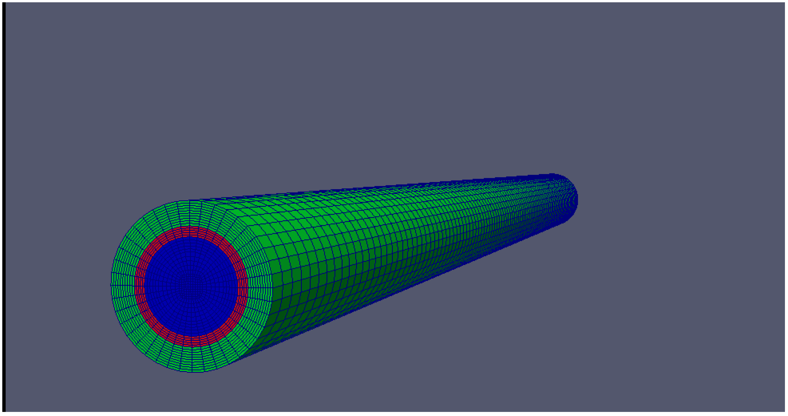
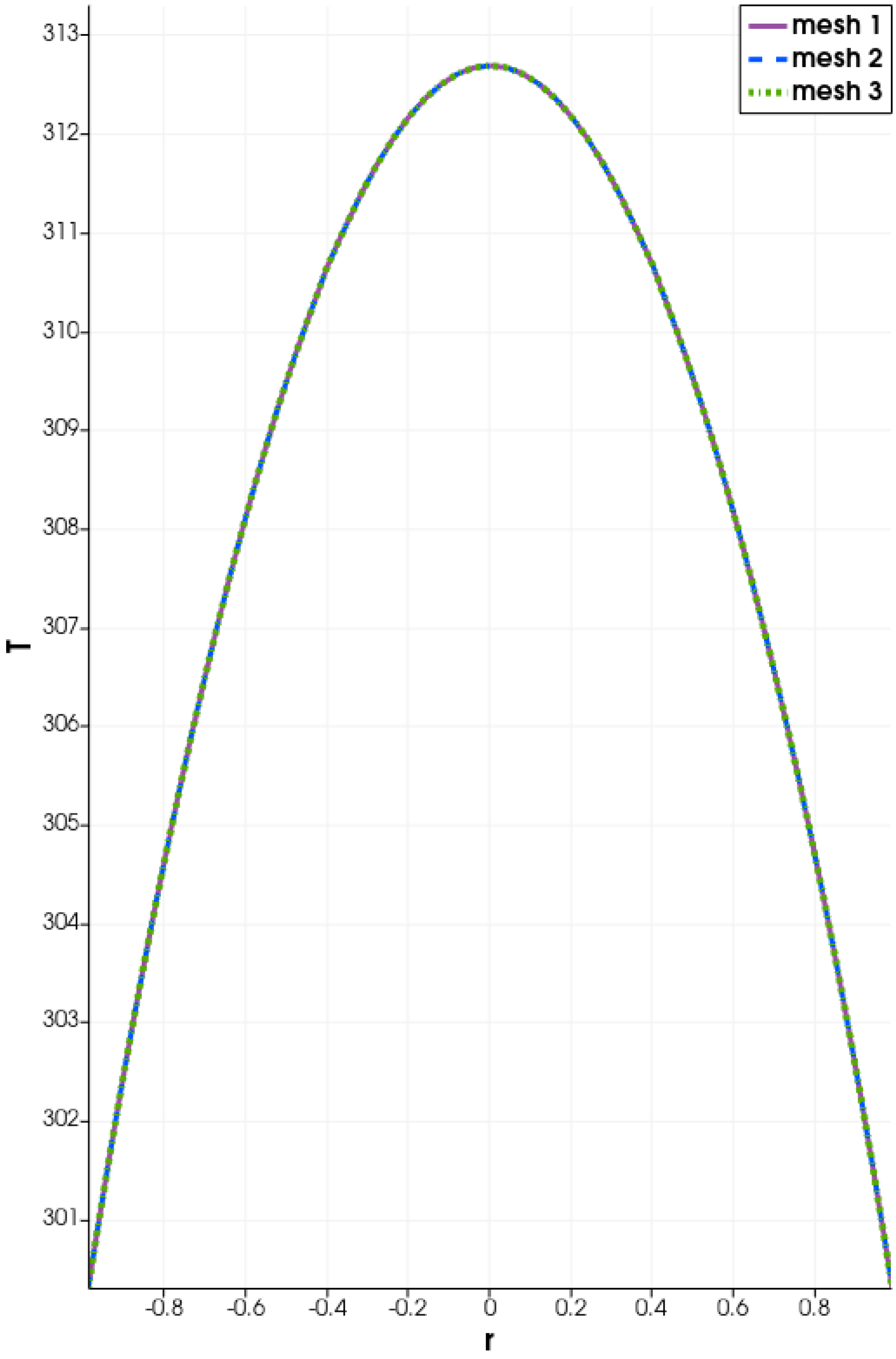
4.1. Mesh Convergence

The mesh independence (or alternatively mesh convergence) in the present simulations is illustrated in Figure 3. The mesh sizes in Figure 3 correspond to the number of computational cells in

Table 1. Mesh sizes corresponding to Figure 3.

mesh 1	120,000 cells
mesh 2	640,000 cells
mesh 3	800,000 cells

.

Given the huge computational costs incurred in running the simulations with such high numbers of computational cells, it is prudent to balance the requirements of mesh convergence, on the one hand, and computational costs, on the other. Figure 3 illustrates mesh independence for the three vastly different mesh sizes. For these reasons, all subsequent simulations in this work are conducted via mesh size 1, i.e., with 120,000 computational cells. It should be remarked that similar mesh independence was observed with much fewer than 120,000 computational cells.

4.2. Dimensionless Parameters

As detailed in [38], it is desirable to report the results with respect to dimensionless parameters. This allows the results to be translated more generally to pipes/geometries of arbitrary size and also to general flow conditions. Results that are based on specific geometric dimensions and specific flow conditions would otherwise be case-specific and not easily generalisable. The relevant dimensionless parameters for the core region are, respectively, the Reynolds number ($R{e}_c$), the Prandtl number ($P{r}_c$), the Deborah number ($De$), the ratio of polymer to total viscosity ($\beta$), and the Giesekus nonlinear parameter ($\epsilon$):

$$\begin{array}{c}\hfill R{e}_c=\frac{{\rho }_c^{*}{U}_{c_0}^{*}{L}^{*}}{{\eta }_c^{*}},P{r}_c=\frac{C_{p_c}^{*}{\eta }_c^{*}}{K_c^{*}},De=\frac{{\lambda }^{*}{U}_{c_0}^{*}}{L^{*}},\beta =\frac{{\eta }_p^{*}}{{\eta }_c^{*}},\epsilon =\frac{L^{*}}{{\eta }_c^{*}{\mu }_c^{*}{U}_{c_0}^{*}}{\alpha }^{*},\end{array}$$

where $U_{c_0}^{*}$ is a reference flow velocity in the core region, say, the constant core-fluid velocity at the inlet. The relevant dimensionless parameters for the shell region are, respectively, the Reynolds and Prandtl numbers, as well as the ratio of nanoparticle to base-fluid thermal conductivities:

$$\begin{array}{c}\hfill R{e}_s=\frac{{\rho }_s^{*}{U}_{s_0}^{*}{L}^{*}}{{\eta }_s^{*}},P{r}_s=\frac{C_{p_s}^{*}{\eta }_s^{*}}{K_f^{*}},\kappa =\frac{K_s^{*}}{K_f^{*}},\end{array}$$

where $U_{s_0}^{*}$ is a reference flow velocity in the shell region, say, the constant shell-fluid velocity at the inlet.

Unless otherwise indicated, the subsequent simulations are carried using the following parameter values:

$$\begin{array}{ccc}\hfill & \mathrm{core}\text{-}\mathrm{fluid}\text{:}\hfill & \hfill R{e}_c=0.6,P{r}_c=0.8,De=0.4,\epsilon =0.2,\beta =0.5,\\ \hfill & \mathrm{shell}\text{-}\mathrm{fluid}\text{:}\hfill & \hfill R{e}_s=90,P{r}_s=3,\\ \hfill & \mathrm{thermal}\text{-}\mathrm{conductivity}\text{:}\hfill & \hfill \kappa =654.16,\aleph =3,\alpha =0.2,A_2=0.5,\phi =0.2.\end{array}$$

The thermal conductivity ratio, $\kappa$, is calculated from the values, $K_s=401$ Wm${}^{-1}$K${}^{-1}$ and $K_f=0.613$ W/(m·K). In the subsequent graphical results, if any of the above parameters are varied, it is understood that the other parameters will be kept at the given values.

4.3. Numerical Validation

The absence of nanoparticles ($\kappa =\aleph =A_2=\phi =0$) reduces the present investigation to that in [38]. Simulations with $\kappa =\aleph =A_2=\phi =0$ give the same results as in [38].

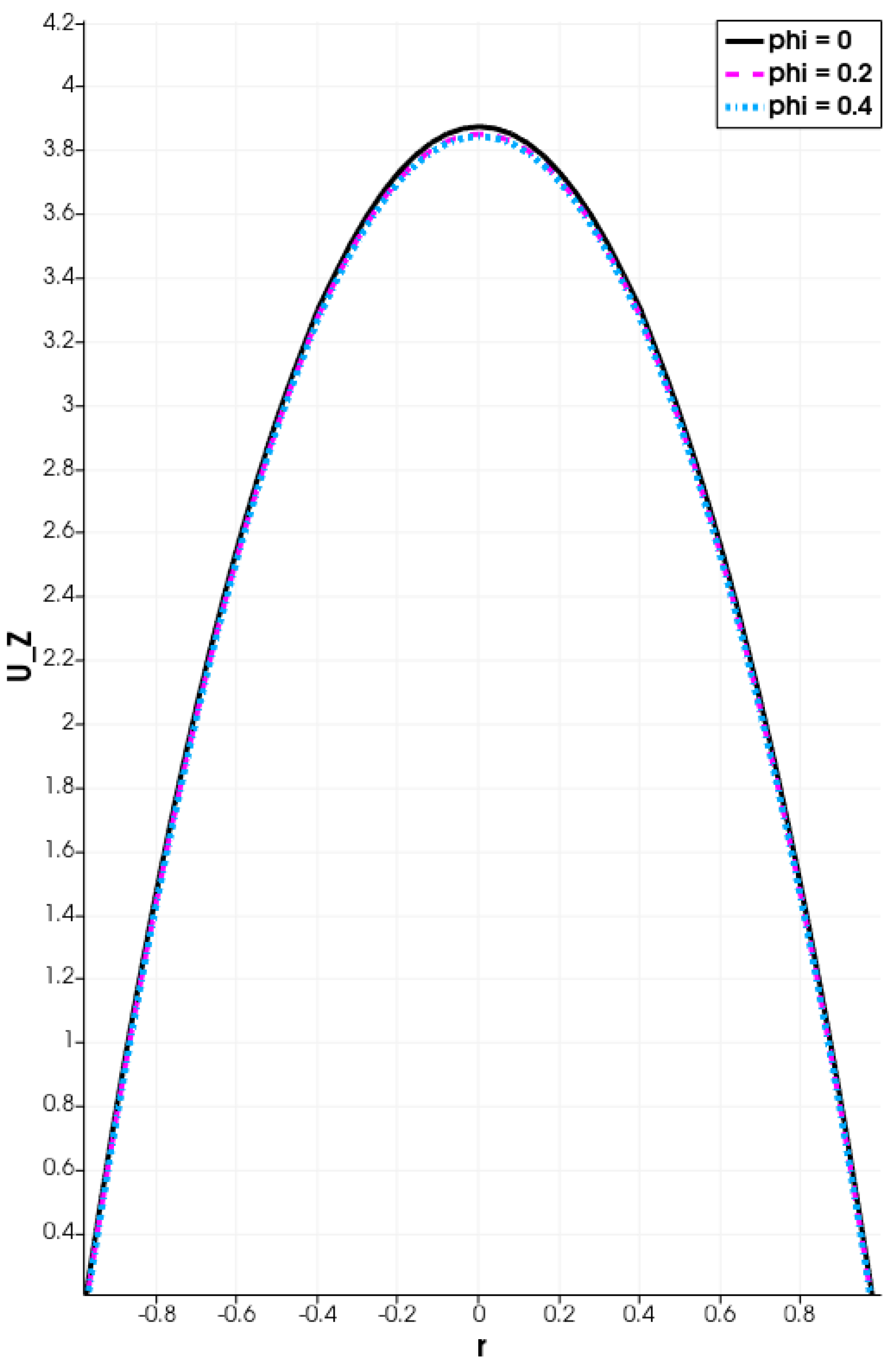
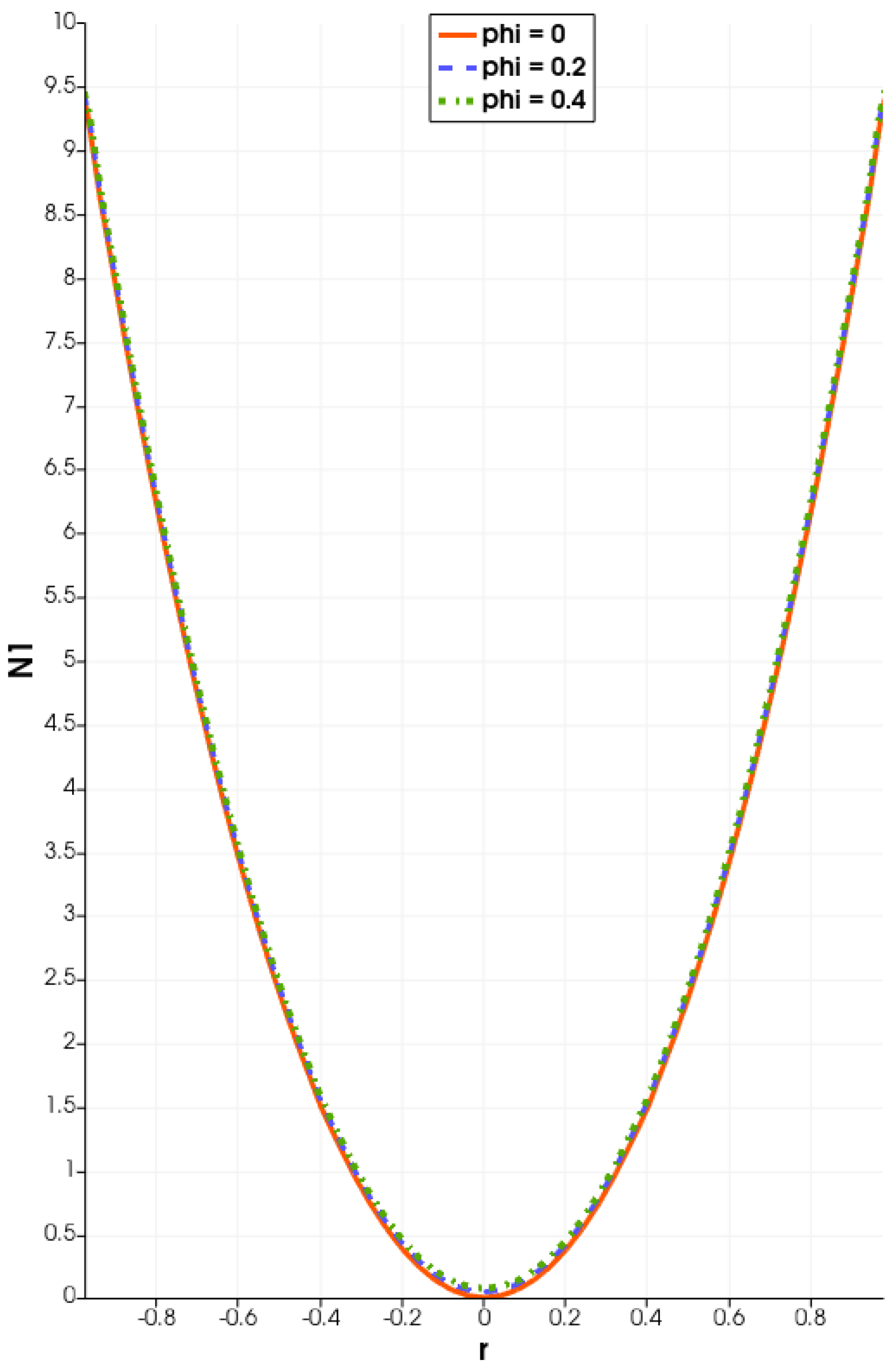
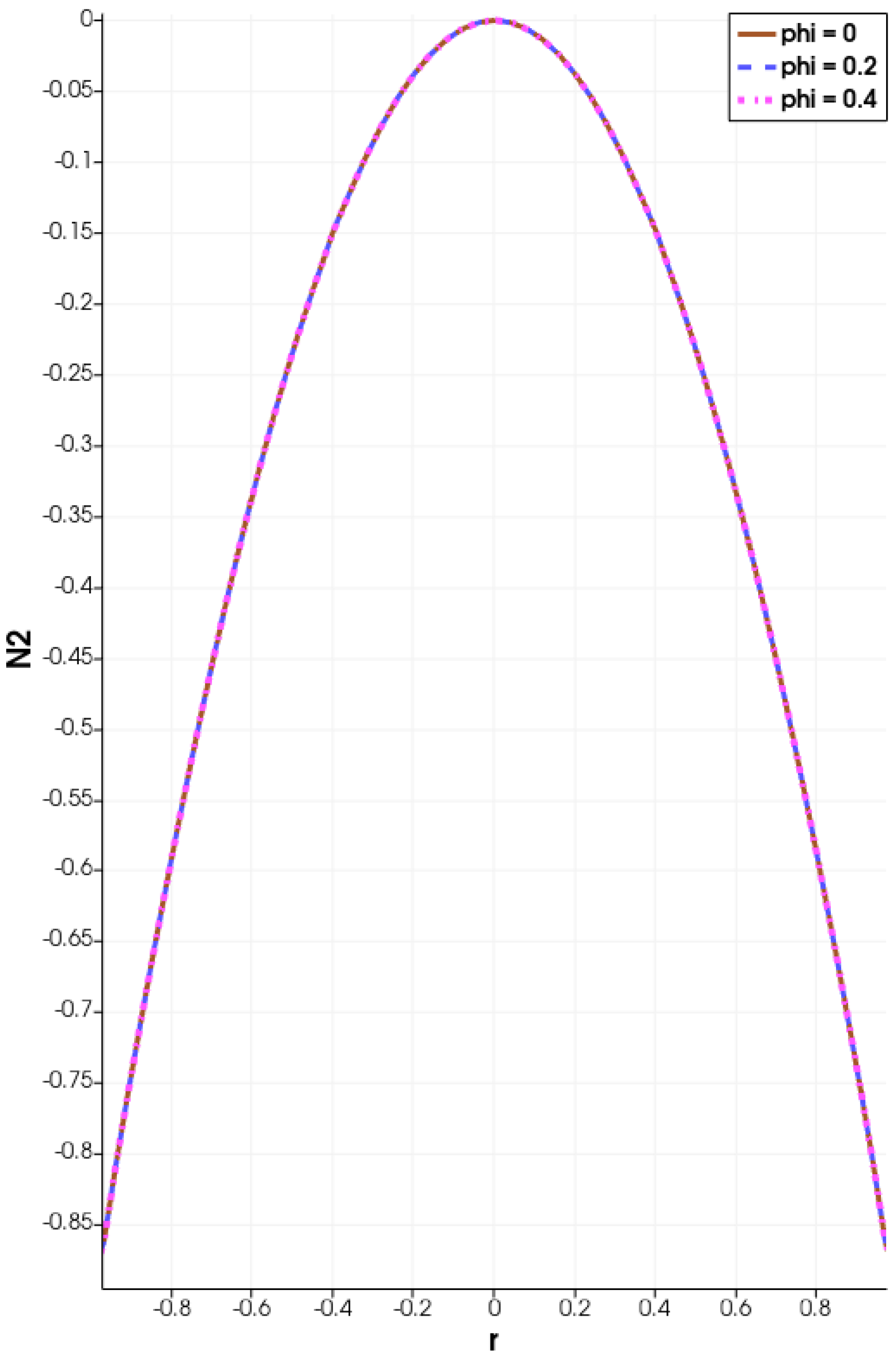
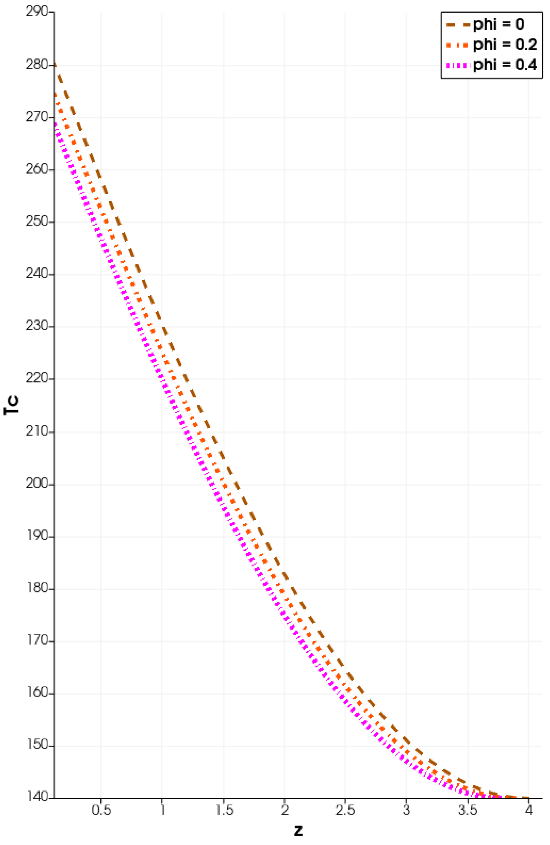
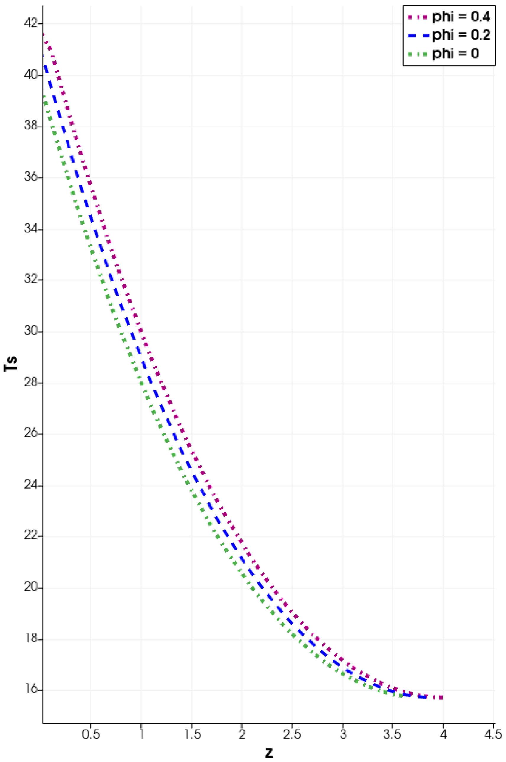
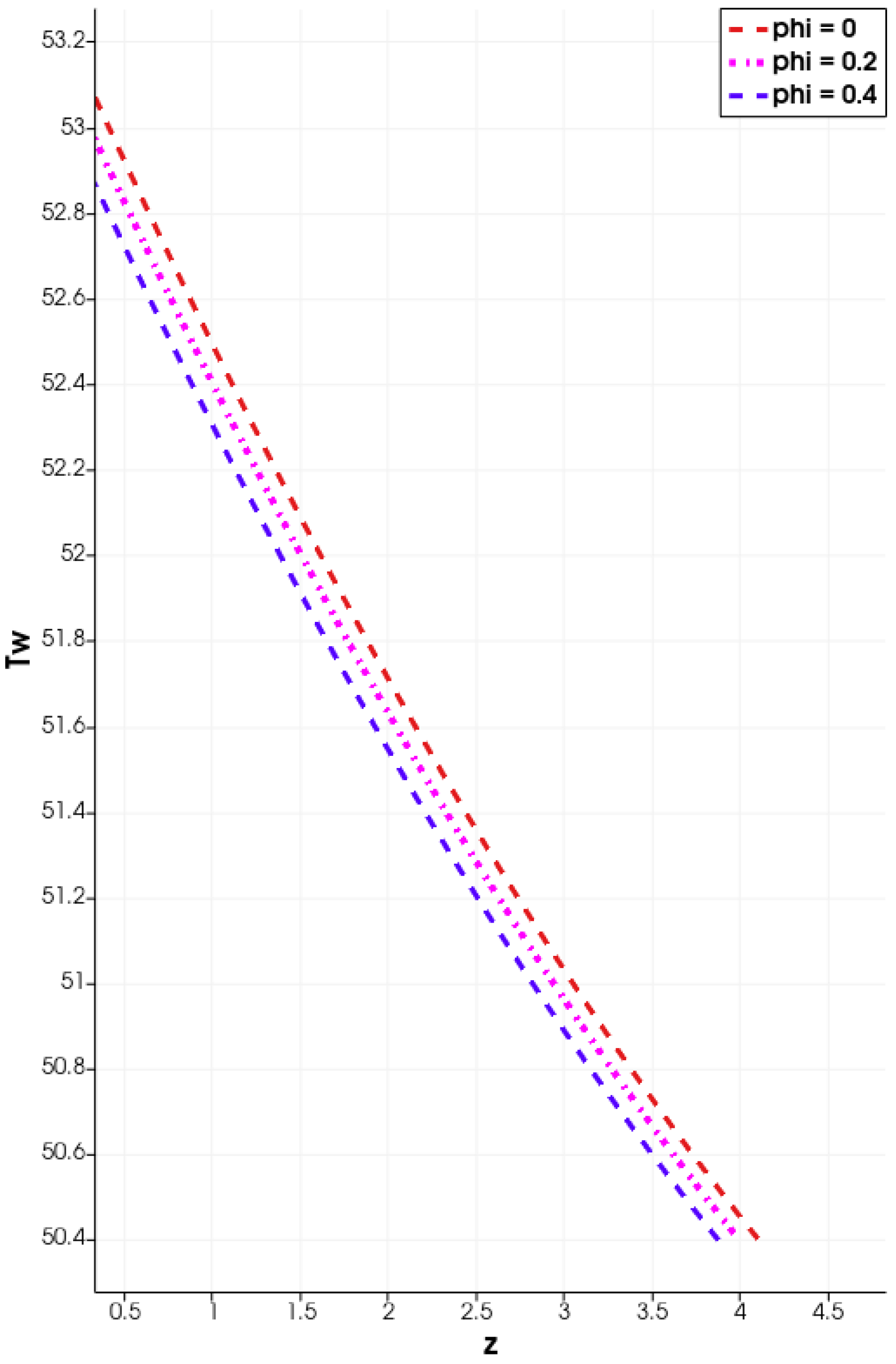
4.4. Response of Flow Variables to Variations in Nanoparticle Volume-Fraction

Figure 4, Figure 5, Figure 6, Figure 7, Figure 8, Figure 9 and Figure 10 demonstrate the effects of varying the nanoparticle volume-fraction, $\phi$, on the flow variables, respectively, the velocity, temperature, pressure, diagonal polymer stress components, and the normal stress differences. The first and second normal-stress differences, $N_1$ and $N_2$, are, respectively, defined as:

$$N_1={\tau }_{zz}-{\tau }_{rr}\mathrm{and}{N}_2={\tau }_{rr}-{\tau }_{\theta \theta }={\tau }_{rr},$$

where the final equality in the second normal stress difference, $N_2$, results from axi-symmetry assumptions, ${\tau }_{\theta \theta }=0$. The first normal-stress difference remains non-negative, $N_1\ge 0$, as required.

The results illustrated in Figure 4, Figure 5, Figure 6, Figure 7, Figure 8, Figure 9 and Figure 10 give the expected parabolic profiles. Of particular note are the important effects of the nanoparticles volume-fraction, $\phi$, on the core-fluid temperature, as shown in Figure 6. The core-fluid temperature decreases as $\phi$ increases. This clearly indicates that increases in the nanoparticles volume-fraction, $\phi$, increase the heat-transfer-rates from the hot core-fluid to the colder shell-nanofluid. Specifically, increases in the nanoparticles volume-fraction, $\phi$, increase the thermal conductivity of the shell-nanofluid, enhancing its coolant characteristics.

Figure 11, Figure 12, Figure 13, Figure 14, Figure 15 and Figure 16 demonstrate the effects of varying the Prandtl number on the core-fluid flow field variables.

The results illustrated in Figure 11, Figure 12, Figure 13, Figure 14, Figure 15 and Figure 16 similarly give the expected parabolic profiles. Of particular note are the expected effects of the Prandtl number on the core-fluid temperature, as shown in Figure 12. The core-fluid temperature decreases as the Prandtl number increases. This is a consequence of the fact that the Prandtl number acts to dampen the strengths of the heat conduction and the heat sources.

Figure 17, Figure 18, Figure 19, Figure 20, Figure 21 and Figure 22 demonstrate the effects of varying the Reynolds number on the core-fluid flow field variables.

The results illustrated in Figure 11, Figure 12, Figure 13, Figure 14, Figure 15 and Figure 16 again give the expected parabolic profiles. Of particular note are the expected effects of the Reynolds number on the core-fluid velocity, as shown in Figure 17. The core-fluid velocity increases as the Reynolds number increases. This follows naturally from the observation that the Reynolds number is directly proportional to the inlet velocity and is also inversely proportional to the fluid viscosity. An increase in the inlet velocity and/or a decrease in the fluid viscosity would act to increase the core-fluid Reynolds number. We also notice from Figure 18 that the core-fluid temperature increases with an increasing Reynolds number.

Figure 23, Figure 24, Figure 25, Figure 26, Figure 27 and Figure 28 demonstrate the effects of varying the Deborah number on the core-fluid flow field variables.

As can be observed from Figure 25, Figure 26, Figure 27 and Figure 28, an increase in the Deborah number increases the elastic effects in the core-fluid. The results illustrated in, say, Figure 25 and Figure 27, demonstrate that the elastic effects are more pronounced closer to the inner pipe walls and away from the pipe centerline.

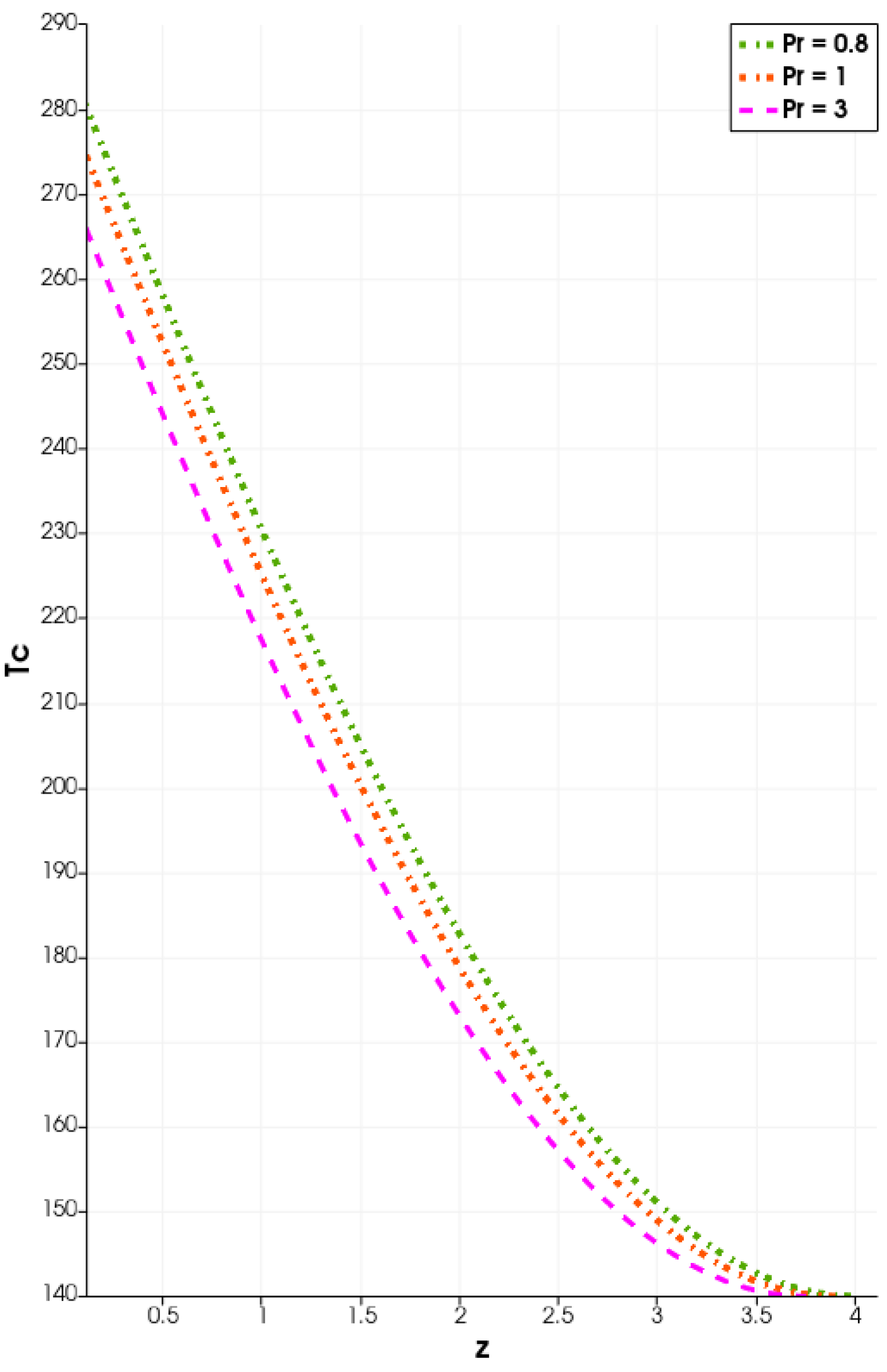
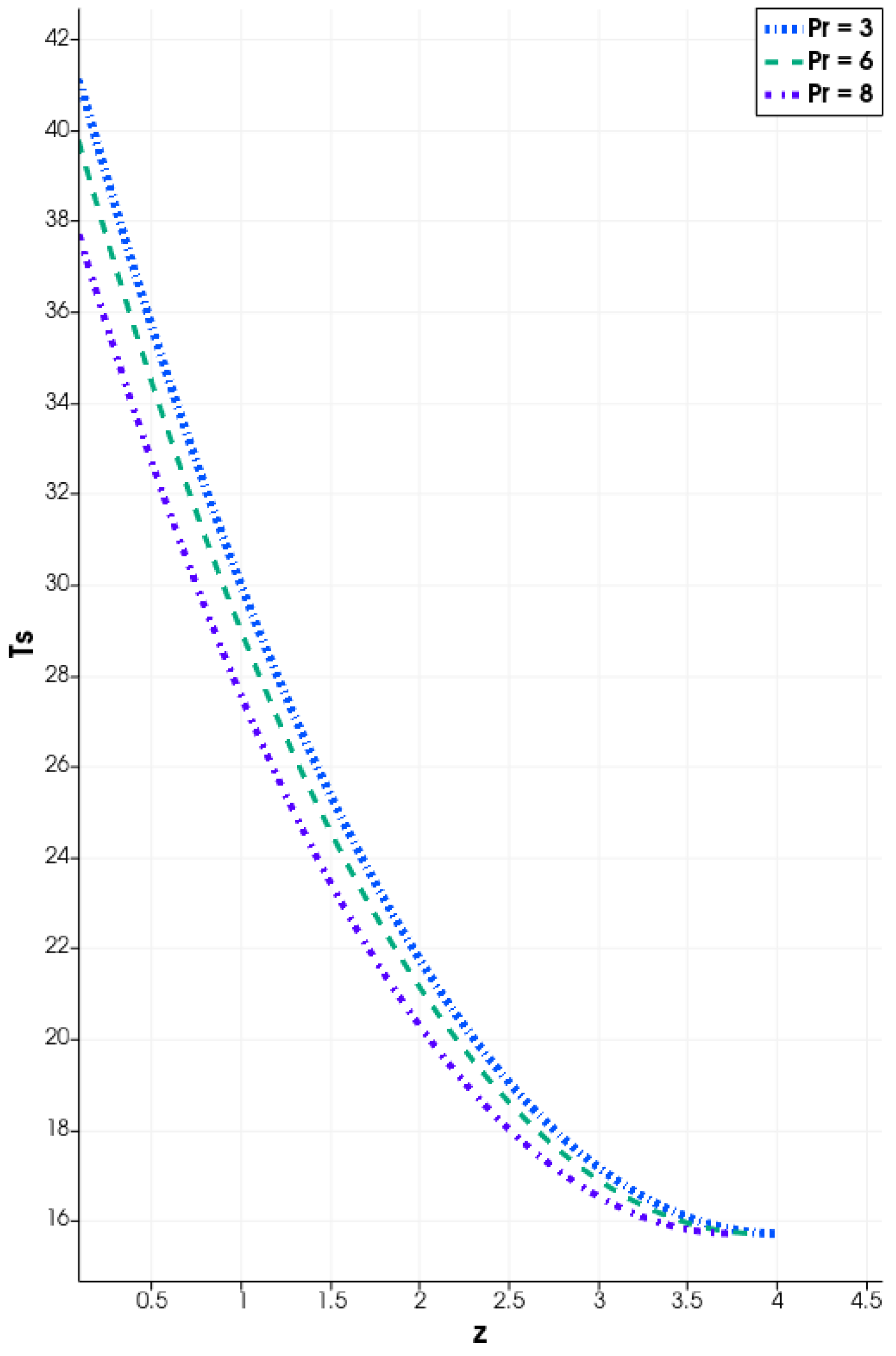
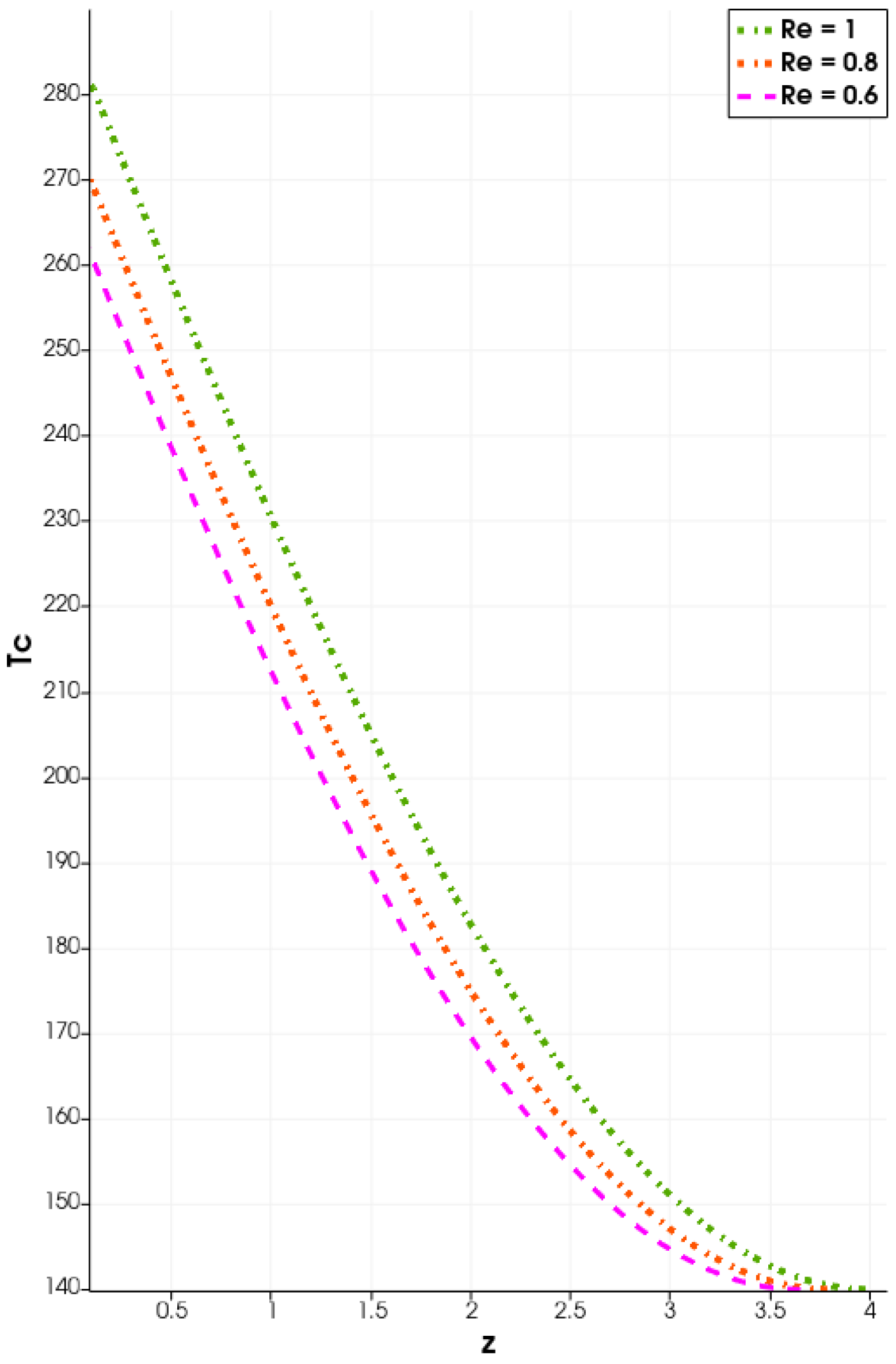
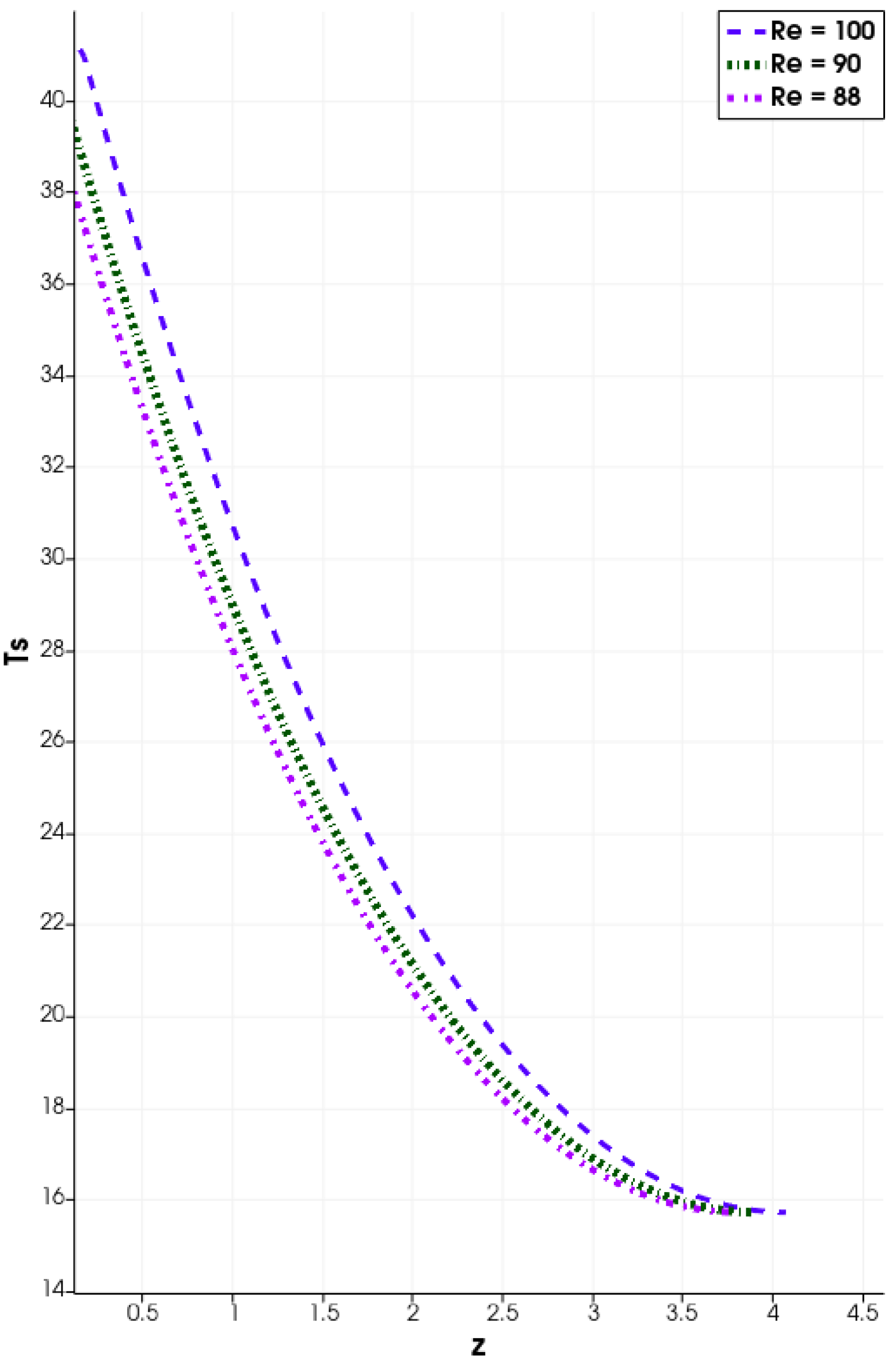
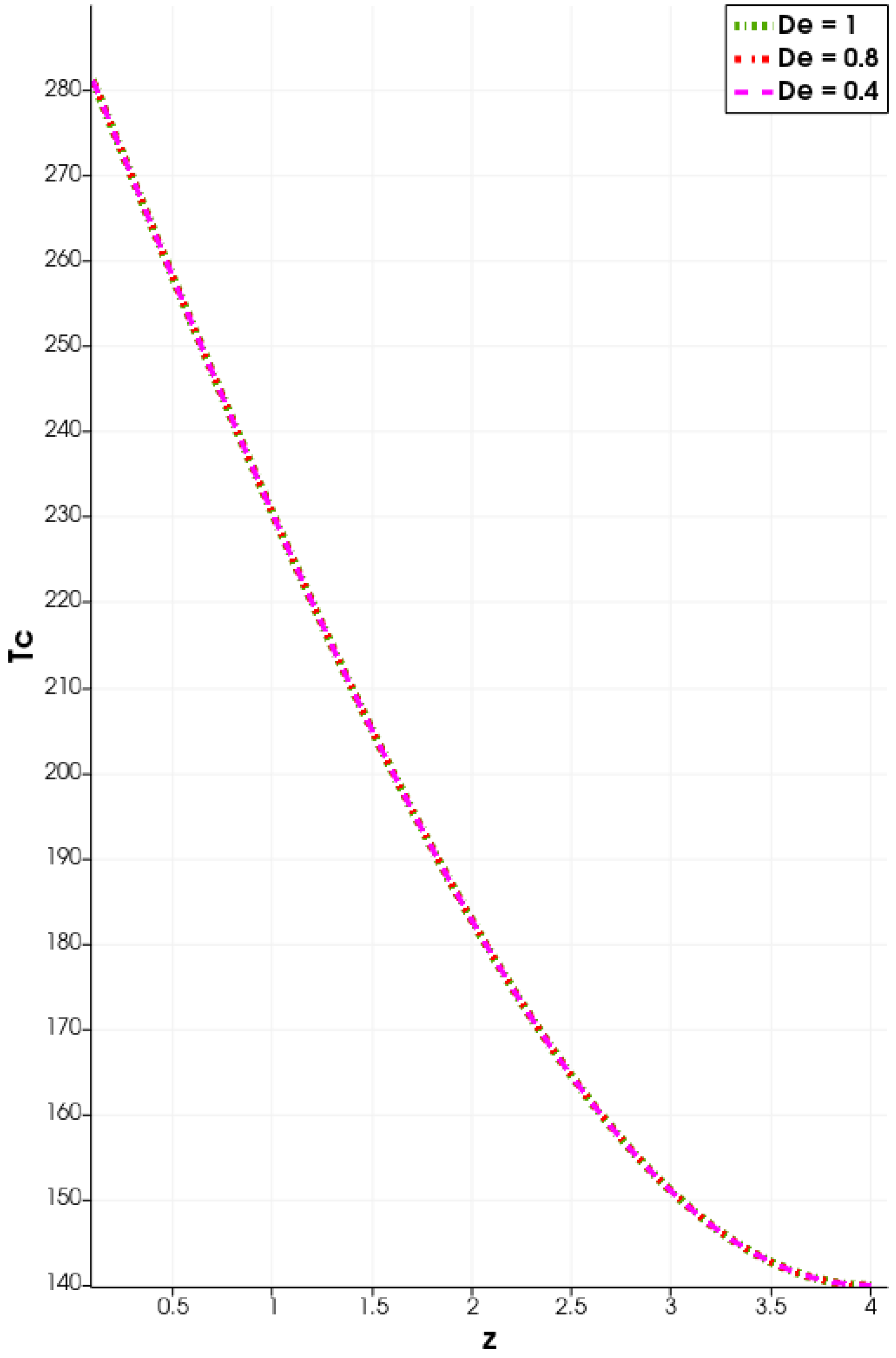
4.5. Response of Flow Variables in the Longitudinal Direction

All the graphical results thus far are presented in the radial direction, across the inner pipe diameter. For this reason, the results have been symmetric about the pipe centerline. It is important to also illustrate the development of the solutions in the longitudinal direction (i.e., the flow direction) in response to variations in flow parameters.

Figure 29 illustrates the behaviour of the core-fluid temperature in the longitudinal direction, in response to variations in the nanoparticle volume-fraction, $\phi$.

The results of Figure 29 show, as expected, that the core-fluid temperature decreases from the initial high values at the inlet to lower values at the outlet. This is the hallmark of a heat exchanger design and function—that a hot fluid is cooled as it flows and interacts with a colder fluid in a connected channel even when the two connected channels containing the hot and cold fluids, respectively, are separated by a solid wall.

Additionally, Figure 29 illustrates, as also shown in the corresponding Figure 6, that the core fluid temperature decreases with increasing nanoparticle volume-fraction, $\phi$. As already explained under Figure 6, this clearly indicates that an increase in the nanoparticles volume-fraction, $\phi$, correspondingly increases the thermal conductivity of the shell-nanofluid, and hence, also increases the heat-exchange characteristics from the hot core-fluid to the colder shell-nanofluid.

Figure 30 illustrates the behaviour of the shell-fluid temperature in the longitudinal direction, in response to variations in the nanoparticle volume-fraction, $\phi$.

The results of Figure 30 show, as expected, that the shell-fluid temperature will increase from the initial low values at the inlet to higher values at the outlet. This is again the hallmark of a heat exchanger design and function—that a coolant fluid is heated as it flows and interacts with a hotter fluid in a connected channel even when the two connected channels, respectively, containing the coolant and hot fluids, are separated by a solid wall.

Figure 31 illustrates the behaviour of the connecting wall temperature in the longitudinal direction, in response to variations in the nanoparticle volume-fraction, $\phi$. The connecting wall temperature would roughly average the core-fluid and shell-fluid temperatures, and hence, the behaviour of the connecting wall temperature largely mirrors the average behavior of the core-fluid and shell-fluid temperatures. Of specific note is that the connecting wall temperature decreases with increasing nanoparticle volume-fraction, $\phi$.

Figure 32 and Figure 33, respectively, illustrate the behaviour of the core-fluid temperature and the shell-fluid temperature, in the longitudinal direction, in response to variations in the Prandtl number, $Pr$. The results are similarly explained as those in Figure 12.

Figure 34 and Figure 35, respectively, illustrate the behaviour of the core-fluid temperature and the shell-fluid temperature, in the longitudinal direction, in response to variations in the Reynolds number, $Re$. The results are similarly explained as those in Figure 18.

Figure 36 illustrates the behaviour of the core-fluid temperature, in the longitudinal direction, in response to variations in the Reynolds number, $Re$. The results are similarly to those in Figure 24 for the radial direction.

5. Concluding Remarks

This study computationally investigates the heat transfer characteristics in a double-pipe counter-flow heat exchanger, with a heated/hot viscoelastic fluid occupying the inner core region and a colder Newtonian-Fluid-Based Nanofluid (NFBN) flowing in the outer shell region. The NFBN is modelled as a single-phase homogenous nanofluid in which the fluid-dynamical and thermodynamical contributions of the embedded nanoparticles are tracked via an appropriate nanoparticle volume-fraction function. A robust numerical methodology based on the finite volume methods (FVM) is employed to solve the complex coupled system of nonlinear PDEs. The FVM algorithms are computationally implemented on the OpenFOAM software platform. The dependence of the field variables on the embedded flow parameters, namely the velocity, temperature, pressure, and polymeric stresses, is explored qualitatively and quantitatively. Specifically, the results illustrate that an increase in the nanoparticle volume-fraction, in the NFBN, leads to enhanced heat exchange characteristics from the hot core fluid to the colder shell NFBN. Significantly, the results illustrate that the use of NFBN as the coolant fluid leads to better heat-transfer characteristics as compared to using an ordinary/conventional (particle-free) Newtonian coolant. The results also demonstrate that the efficacy of the NFBN as a coolant is enhanced with increasing nanoparticle volume-fraction. The effects of the volume fraction parameter and Prandtl number were observed to be insignificant on the velocity field, pressure field, and polymer-stress components. Similarly, the effects of the Deborah number were observed to be insignificant on the velocity and temperature fields.

References

1. Eastman, J.A.; Choi, U.S.; Thompson, L.J.; Lee, S. Enhanced thermal conductivity through the development of nanofluids. Mater Res. Soc. Symp. Proc. 1996, 457, 3–11. [Google Scholar] [CrossRef] [Green Version]
2. Liu, M.S.; Lin, M.C.C.; Huang, I.T.; Wang, C.C. Enhancement of thermal conductivity with CuO for nanofluids. Chem. Eng. Technol. 2006, 29, 72–77. [Google Scholar] [CrossRef]
3. Hwang, Y.; Par, H.S.K.; Lee, J.K.; Jung, W.H. Thermal conductivity and lubrication characteristics of nanofluids. Curr. Appl. Phys. 2006, 6 (Suppl. 1), 67–71. [Google Scholar] [CrossRef]
4. Yu, W.; Xie, H.; Chen, L.; Li, Y. Investigation of thermal conductivity and viscosity of ethylene glycol based ZnO nanofluid. Thermochim. Acta 2009, 491, 92–96. [Google Scholar] [CrossRef]
5. Mintsa, H.A.; Roy, G.; Nguyen, C.T.; Doucet, D. New temperature dependent thermal conductivity data for water-based nanofluids. Int. J. Therm. Sci. 2009, 48, 363–371. [Google Scholar] [CrossRef]
6. Murshed, S.M.S.; Leong, K.C.; Yang, C. Enhanced thermal conductivity of TiO2–water based nanofluids. Int. J. Therm. Sci. 2005, 44, 367–373. [Google Scholar] [CrossRef]
7. Patel, H.E.; Das, S.K.; Sundararajan, T.; Nair, A.S.; George, B.; Pradeep, T. Thermal conductivities of naked and monolayer protected metal nanoparticle based nanofluids: Manifestation of anomalous enhancement and chemical effects. Appl. Phys. Lett. 2003, 83, 2931–2933. [Google Scholar] [CrossRef] [Green Version]
8. Xuan, Y.; Li, Q. Heat transfer enhancement of nanofluids. Int. J. Heat Fluid Flow 2000, 21, 58–64. [Google Scholar] [CrossRef]
9. Assael, M.J.; Metaxa, I.N.; Kakosimos, K.; Constantinou, D. Thermal Conductivity of Nanofluids—Experimental and Theoretical. Int. J. Thermophys. 2006, 27, 999–1017. [Google Scholar] [CrossRef]
10. Philip, J.; Laskar, J.M.; Raj, B. Magnetic field induced extinction of light in a suspension of Fe3O4 nanoparticles. Appl. Phys. Lett. 2008, 92, 221911. [Google Scholar] [CrossRef]
11. Abu-Nada, E.; Oztop, H.F. Numerical analysis of Al2O3/Water nanofluids natural convection in a wavy walled cavity. Numer. Heat Transf. A Appl. 2011, 59, 403–419. [Google Scholar] [CrossRef]
12. Yurddaş, A.; Çerçi, Y. Numerical analysis of heat transfer in a flat-plate solar collector with nanofluids. Heat Transf. Res. 2017, 48, 681–714. [Google Scholar] [CrossRef]
13. Kamyar, A.; Saidur, R.; Hasanuzzaman, M. Application of Computational Fluid Dynamics (CFD) for nanofluids. Int. J. Heat Mass Transf. 2012, 55, 4104–4115. [Google Scholar] [CrossRef]
14. Moraveji, M.K.; Darabi, M.; Haddad, S.M.H.; Davarnejad, R. Modeling of convective heat transfer of a nanofluid in the developing region of tube flow with computational fluid dynamics. Int. Commun. Heat Mass Transf. 2011, 38, 1291–1295. [Google Scholar] [CrossRef]
15. Hwang, Y.; Lee, J.K.; Lee, C.H.; Jung, Y.M.; Cheong, S.I.; Lee, C.G.; Ku, B.C.; Jang, S.P. Stability and thermal conductivity characteristics of nanofluids. Thermochim. Acta 2007, 455, 70–74. [Google Scholar] [CrossRef]
16. Sharma, P.; Baek, I.; Cho, T.; Park, S.; Bong, K. Enhancement of thermal conductivity of ethylene glycol based silver nanofluids. Powder Technol. 2011, 208, 7–19. [Google Scholar] [CrossRef]
17. Das, S.K.; Putra, N.; Thiesen, P.; Roetzel, W. Temperature dependence of thermal conductivity enhancement for nanofluids. J. Heat Transf. ASME 2015, 125, 567–574. [Google Scholar] [CrossRef]
18. Özerinç, S.; Kalaç, S.; Yazicioǧlu, A.G. Enhanced thermal conductivity of nanofluids: A state-of-the-art review. Microfluid. Nanofluid. 2010, 8, 145–170. [Google Scholar] [CrossRef]
19. Terekhov, V.I.; Kalinina, S.V.; Lemanov, V.V. The mechanism of heat transfer in nanofluids: State of the art (review). Part 1. Synthesis and properties of nanofluids. Thermophys. Aeromech. 2010, 17, 1–14. [Google Scholar] [CrossRef]
20. Keblinski, P.; Phillpot, S.R.; Choi, S.U.; Eastman, J.A. Mechanisms of heat flow in suspensions of nano-sized particles (nanofluids). Int. J. Heat Mass Transf. 2002, 45, 855–863. [Google Scholar] [CrossRef]
21. Mahyari, A.A.; Karimipour, A.; Afrand, M. Effects of dispersed added graphene oxide-silicon carbide nanoparticles to present a statistical formulation for the mixture thermal properties. Phys. A Stat. Mech. Appl. 2019, 521, 98–112. [Google Scholar] [CrossRef]
22. Pang, C.; Jung, J.Y.; Kang, Y.T. Aggregation based model for heat conduction mechanism in nanofluids. Int. J. Heat Mass Transf. 2014, 72, 392–399. [Google Scholar] [CrossRef]
23. Lee, S.; Choi, S.U.S.; Li, S.; Eastman, J.A. Measuring thermal conductivity of fluids containing oxide nanoparticles. J. Heat Transf. 1999, 121, 280–289. [Google Scholar] [CrossRef]
24. Wang, X.; Xu, X.; Choi, S.U.S. Thermal conductivity of nanoparticle-fluid mixture. J. Thermophys. Heat Transf. 1999, 13, 474–480. [Google Scholar] [CrossRef]
25. Masuda, H.; Ebata, A.; Teramea, K.; Hishinuma, N. Alteration of thermal conductivity and viscosity of liquid by dispersing ultra-fine particles. Netsu Bussei 1993, 4, 227–233. [Google Scholar] [CrossRef]
26. Grimm, A. Powdered Aluminum-Containing Heat Transfer Fluids. German Patent DE 4131516A1, 8 April 1993. [Google Scholar]
27. Eastman, J.A.; Choi, S.U.S.; Li, S.; Yu, W.; Thompson, L.J. Anomalously Increased Effective Thermal Conductivities Containing Copper Nanoparticles. Appl. Phys. Lett. 2001, 78, 718–720. [Google Scholar] [CrossRef]
28. Ding, Y.; Alias, H.; Wen, D.; Williams, R.A. Heat transfer of aqueous suspensions of carbon nanotubes (CNT nanofluids). Int. J. Heat Mass Transf. 2006, 49, 240. [Google Scholar] [CrossRef]
29. Heris, S.Z.; Esfahany, M.N.; Etemad, S.G. Experimental investigation of convective heat transfer of Al2O3/water nanofluid in circular tube. Int. J. Heat Fluid Flow 2007, 28, 203–210. [Google Scholar] [CrossRef]
30. Xuan, Y.; Li, Q. Investigation on Convective Heat Transfer and Flow Features of Nanofluids. J. Heat Transf. 2003, 1, 151–155. [Google Scholar] [CrossRef] [Green Version]
31. Li, Q.; Xuan, Y. Convective Heat Transfer and Flow Characteristics of Cu-Water Nanofluid. Sci. China (Ser. E) 2002, 45, 408–416. [Google Scholar]
32. Khan, I.; Chinyoka, T.; Gill, A. Computational analysis of the dynamics of generalized-viscoelastic-fluid-based nano-fluids subject to exothermic-reaction in shear-flow. J. Nanofluids 2022, 11, 1–13. [Google Scholar]
33. Khan, I.; Chinyoka, T.; Gill, A. Dynamics of Non-Isothermal Pressure-Driven Flow of Generalized Viscoelastic-Fluid-Based Nanofluids in a Channel. Math. Probl. Eng. 2022, 22, 1–17. [Google Scholar] [CrossRef]
34. Kristiawan, B.; Rifái, A.I.; Enoki, K.; Wijayanta, A.T.; Miyazaki, T. Enhancing the thermal performance of TiO2/water nanofluids flowing in a helical microfin tube. Powder Technol. 2020, 376, 254–262. [Google Scholar] [CrossRef]
35. Kondaraju, S.; Jin, E.K.; Lee, J.S. Investigation of heat transfer in turbulent nanofluids using direct numerical simulation. Phys. Rev. E 2010, 81, 016304. [Google Scholar] [CrossRef]
36. Kalteh, M.; Abbassi, A.; Saffar-Avval, M.; Harting, J. Eulerian–Eulerian two-phase numerical simulation of nanofluid laminar forced convection in a microchannel. Int. J. Heat Fluid Flow 2010, 32, 107–116. [Google Scholar] [CrossRef]
37. Chinyoka, T. Viscoelastic effects in double-pipe single-pass counterflow heat ex-changers. Int. J. Numer. Methods Fluids 2008, 59, 667–690. [Google Scholar]
38. Mavi, A.; Chinyoka, T.; Gill, A. Finite volume computational analysis of the heat transfer characteristic in a double-cylinder counter-flow heat exchanger with viscoelastic fluids. 2022; under review. [Google Scholar]
39. Pranowo; Makarim, D.A.; Suami, A.; Wijayanta, A.T.; Kobayashi, N.; Itaya, Y. Marangoni convection within thermosolute and absorptive aqueous LiBr solution. Int. J. Heat Mass Transf. 2022, 188, 122621. [Google Scholar] [CrossRef]
40. Weller, H.G.; Tabor, G.; Jasak, H.; Fureby, C. A Tensorial Approach to Computational Continuum Mechanics Using Object Orientated Techniques. Comput. Phys. 1998, 12, 620–631. [Google Scholar] [CrossRef]
41. Pimenta, F.; Alves, M.A. rheoTool. 2016. Available online: https://github.com/fppimenta/rheoTool (accessed on 8 February 2022).
42. Favero, J.L.; Secchi, A.R.; Cardozo, N.S.M.; Jasak, H. Viscoelastic flow analysis using the software OpenFOAM and differential constitutive equations. J. Non–Newton. Fluid Mech. 2010, 165, 1625–1636. [Google Scholar] [CrossRef]
43. Abuga, J.G.; Chinyoka, T. Benchmark solutions of the stabilized computations of flows of fluids governed by the Rolie-Poly constitutive model. J. Phys. Commun. 2020, 4, 015024. [Google Scholar] [CrossRef]
44. Abuga, J.G.; Chinyoka, T. Numerical Study of Shear Banding in Flows of Fluids Governed by the Rolie-Poly Two-Fluid Model via Stabilized Finite Volume Methods. Processes 2020, 8, 810. [Google Scholar] [CrossRef]
45. Nyandeni, Z.; Chinyoka, T. Computational aeroacoustic modeling using hybrid Reynolds averaged Navier–Stokes/large-eddy simulations methods with modified acoustic analogies. Int. J. Numer. Methods Fluids 2021, 93, 2611–2636. [Google Scholar] [CrossRef]
46. Meburger, S.; Niethammer, M.; Bothe, D.; Schäfer, M. Numerical simulation of non-isothermal viscoelastic flows at high Weissenberg numbers using a finite volume method on general unstructured meshes. J. Non–Newton. Fluid Mech. 2021, 287, 104–451. [Google Scholar] [CrossRef]
47. Habla, F.; Woitalka, A.; Neuner, S.; Hinrichsen, O. Development of a methodology for numerical simulation of non-isothermal viscoelastic fluid flows with application to axisymmetric 4: 1 contraction flows. Chem. Eng. J. 2012, 207, 772–784. [Google Scholar] [CrossRef]
48. Peters, G.W.M.; Baaijens, F.P.T. Modelling of non-isothermal viscoelastic flows. J. Non–Newton. Fluid Mech. 1997, 74, 205–224. [Google Scholar] [CrossRef] [Green Version]
49. Wapperom, M.A.H.P.; van der Zanden, P.P.M. A numerical method for steady and nonisothermal viscoelastic fluid flow for high deborah and pclet numbers. Rheol. Acta 1998, 37, 73–88. [Google Scholar] [CrossRef]
50. Hamilton, R.L.; Crosser, O.K. Thermal conductivity of heterogeneous two-component systems. Ind. Eng. Chem. 1962, 1, 187–191. [Google Scholar] [CrossRef]
51. Favero, J.L. Viscoelastic Flow Simulation in Openfoam: Presentation of the Viscoelasticfluidfoam Solver Technical Report, Universidade Federal do Rio Grande do Sul-Department of Chemical Engineering. 2009. Available online: http://powerlab.fsb.hr/ped/kturbo/OpenFOAM/slides/viscoelasticFluidFoam.pdf (accessed on 8 February 2022).
52. Fattal, R.; Kupferman, R. Constitutive laws for the matrix-logarithm of the con-formation tensor. J. Non–Newton. Fluid Mech. 2004, 123, 281–285. [Google Scholar] [CrossRef]
53. Fattal, R.; Kupferman, R. Finite element methods for calculation of steafy viscoealstic flow using constitutive equation with a Newtonian viscosity. J. Non–Newton. Fluid Mech. 1990, 36, 159–192. [Google Scholar]
54. Guénette, R.; Fortin, M. A new mixed finite element method for computing viscoelastic flows. J. Non–Newton. Fluid Mech. 1995, 60, 27–52. [Google Scholar] [CrossRef]
55. Amoreira, L.J.; Oliveira, P.J. Comparison of Different Formulations for the Numerical Calculation of Unsteady Incompressible Viscoelastic Fluid Flow. Adv. Appl. Math. Mech. 2010, 27, 483–502. [Google Scholar]
56. Issa, R.I. Solution of the implicitly discretised fluid flow equations by operator-splitting. J. Comp. Phys. 1986, 62, 40–65. [Google Scholar] [CrossRef]
Figure 1. Schematics of the model problem.
Applsci 12 05475 g001
Figure 2. Computational mesh for the double-pipe geometry.
Applsci 12 05475 g002
Figure 3. Illustration of mesh independence.
Applsci 12 05475 g003
Figure 4. Effects of nanoparticle volume-fraction, φ , on the core-fluid velocity.
Applsci 12 05475 g004
Figure 5. Effects of nanoparticle volume-fraction, φ , on the core-fluid pressure.
Applsci 12 05475 g005
Figure 6. Effects of nanoparticle volume-fraction, φ , on the core-fluid temperature.
Applsci 12 05475 g006
Figure 7. Effects of nanoparticle volume-fraction, φ , on the diagonal stress component, τ r r .
Applsci 12 05475 g007
Figure 8. Effects of nanoparticle volume-fraction, φ , on the diagonal stress component, τ z z .
Applsci 12 05475 g008
Figure 9. Effects of nanoparticle volume-fraction, φ , on the first normal stress difference, N 1 .
Applsci 12 05475 g009
Figure 10. Effects of nanoparticle volume-fraction, φ , on the second normal stress difference, N 2 .
Applsci 12 05475 g010
Figure 11. Effects of Prandtl number, P r , on the core-fluid velocity.
Applsci 12 05475 g011
Figure 12. Effects of Prandtl number, P r , on the core-fluid temperature.
Applsci 12 05475 g012
Figure 13. Effects of Prandtl number, P r , on the diagonal stress component, τ r r .
Applsci 12 05475 g013
Figure 14. Effects of Prandtl number, P r , on the diagonal stress component, τ z z .
Applsci 12 05475 g014
Figure 15. Effects of Prandtl number, P r , on the first normal stress difference, N 1 .
Applsci 12 05475 g015
Figure 16. Effects of Prandtl number, P r , on the second normal stress difference, N 2 .
Applsci 12 05475 g016
Figure 17. Effects of Reynolds number, R e , on the core-fluid velocity.
Applsci 12 05475 g017
Figure 18. Effects of Reynolds number, R e , on the core-fluid temperature.
Applsci 12 05475 g018
Figure 19. Effects of Reynolds number, R e , on the diagonal stress component, τ r r .
Applsci 12 05475 g019
Figure 20. Effects of Reynolds number, R e , on the diagonal stress component, τ z z .
Applsci 12 05475 g020
Figure 21. Effects of Reynolds number, R e , on the first normal stress difference, N 1 .
Applsci 12 05475 g021
Figure 22. Effects of Reynolds number, R e , on the second normal stress difference, N 2 .
Applsci 12 05475 g022
Figure 23. Effects of Deborah number, D e , on the core-fluid velocity.
Applsci 12 05475 g023
Figure 24. Effects of Deborah number, D e , on the core-fluid temperature.
Applsci 12 05475 g024
Figure 25. Effects of Deborah number, D e , on the diagonal stress component, τ r r .
Applsci 12 05475 g025
Figure 26. Effects of Deborah number, D e , on the diagonal stress component, τ z z .
Applsci 12 05475 g026
Figure 27. Effects of Deborah number, D e , on the first normal stress difference, N 1 .
Applsci 12 05475 g027
Figure 28. Effects of Deborah number, D e , on the second normal stress difference, N 2 .
Applsci 12 05475 g028
Figure 29. Effects of nanoparticles volume-fraction φ on the core-fluid temperature. Fluid moving from inlet at z = 0 to outlet at z = 4 , i.e., flow direction is from left to right (⟶).
Applsci 12 05475 g029
Figure 30. Effects of nanoparticles volume-fraction φ on shell-fluid temperature. Fluid moving from inlet at z = 4 to outlet at z = 0 , i.e., flow direction is from right to left (⟵).
Applsci 12 05475 g030
Figure 31. Effects of nanoparticles volume-fraction, φ , on the connecting wall temperature.
Applsci 12 05475 g031
Figure 32. Effects of Prandtl number, P r , on core-fluid temperature. Fluid moving from inlet at z = 0 to outlet at z = 4 , i.e., flow direction is from left to right (⟶).
Applsci 12 05475 g032
Figure 33. Effects of Prandtl number, P r , on shell-fluid temperature. Fluid moving from inlet at z = 4 to outlet at z = 0 , i.e., flow direction is from right to left (⟵).
Applsci 12 05475 g033
Figure 34. Effects of Reynolds number, R e , on core-fluid temperature. Fluid moving from inlet at z = 0 to outlet at z = 4 , i.e., flow direction is from left to right (⟶).
Applsci 12 05475 g034
Figure 35. Effects of Reynolds number, R e , on the shell-fluid temperature. Fluid moving from inlet at z = 4 to outlet at z = 0 , i.e., flow direction is from right to left (⟵).
Applsci 12 05475 g035
Figure 36. Effects of Deborah number, D e , on the core-fluid temperature. Fluid moving from inlet at z = 0 to outlet at z = 4 , i.e., flow direction is from left to right (⟶).
Applsci 12 05475 g036