Physical Survey of Thermally Heated Non-Newtonian Jeffrey Fluid in a Ciliated Conduit Having Heated Compressing and Expanding Walls

Abstract

An analytical study is reported that highlights the physical aspects for a heated non-Newtonian Jeffrey liquid in a duct possessing sinusoidally moving ciliated walls. A comprehensive and specific convection analysis is conveyed for this ciliated elliptic duct problem by considering the viscous dissipation effects. The dimensional mathematical problem under consideration is transformed into its dimensionless form by means of appropriate and useful transformations. Then, velocity and temperature equations are exactly evaluated with given boundary conditions. The velocity profile is integrated over the elliptic cross-section and exact mathematical solution is obtained for the pressure gradient. Moreover, the distinct physical flow properties combined with the convection heat transfer phenomenon are discussed in detail through graphical outcomes. The illustrative streamline description shows an enhancing closed contour size with increasing $Q$ (dimensionless flow rate).

1. Introduction

The computational interpretation of convection in elliptic conduits is an important and worthy topic of recent interest for many researchers. A huge mathematical literature exists on the distinct flow characteristics and heat convection problems for elliptic ducts. Abdel-Wahed [1] disclosed the experimental model of convection in elliptic conduits. Maia et al. [2] reported the heat flux for a heated liquid in an elliptic domain geometry. Ragueb et al. [3] presented the mathematical interpretation of non-Newtonian forced convection flow in an elliptic duct. Our main intention, in this work, is to analyse the convection phenomenon in an elliptic domain having heated deformable walls.

Peristalsis mainly deals with the flow problems that involve the movement of channel walls to propagate the flow. Its comprehensive and broad range of practical applications in engineering problems make it a worthy topic of interest. Barton and Raynor [4] disclosed the mathematical study of peristaltic flow and it is basically propagated in the tube due to deformation of the tube’s walls. Bohme and Friedrich [5] reported the mathematical analysis that deals with the non-Newtonian peristaltic flow problem. The peristaltic flow phenomenon, due to its practical field applications, is not just confined to cylindrical geometries. Many researchers reported recent research on peristaltic flow in view of multiple liquids and geometry domain models, such as non-uniform tubes [6,7], diverging tube [8,9], curved tube [10,11], rectangular ducts [12,13,14] and elliptic duct [15].

The metachronal wave effect on peristaltic flow is also mathematically investigated by many researchers. This metachronal wave is mainly generated due to rhythmic and sequential beating of cilia (hair-like tiny structures). The development of metachronal wave due to cilia also plays a key role in the flow propagation. Akbar and Butt [16] disclosed the mathematical interpretation of the cilia-driven peristaltic flow of non-Newtonian fluids. Akbar et al. [17] scrutinized the transportation in a sinusoidal passage with cilia beating. Saleem et al. [18] disclosed the flow in a bent tube with effects of cilia beating and distinct physical properties of peristalsis. Butt et al. [19] mathematically modelled the propulsion of Phan Thien Tanner non-Newtonian fluid in a sinusoidal pipe with the combined effects of cilia beating. Some recent studies on polymeric flow problems with weak form solution approaches are provided [20,21,22].

The current assessment is done to mathematically interpret the peristaltic flow with convection for a non-Newtonian Jeffrey fluid in a ciliated elliptical conduit. The viscous dissipation effect is also integrated in the heat equation to provide a comprehensive interpretation of heat transfer for this convection heat transfer problem. A set of useful transformations and dimensionless parameters are employed to avail the dimensionless form of the mathematical problem. We developed exact results for pressure gradient, temperature and velocity. The distinct physical properties and heat convection aspects of this developed problem are analysed in detail through graphical outcomes. The increasing value of $Q$ results in an enhanced contour size but a decline is observed in number of contours, as shown in streamline graphs.

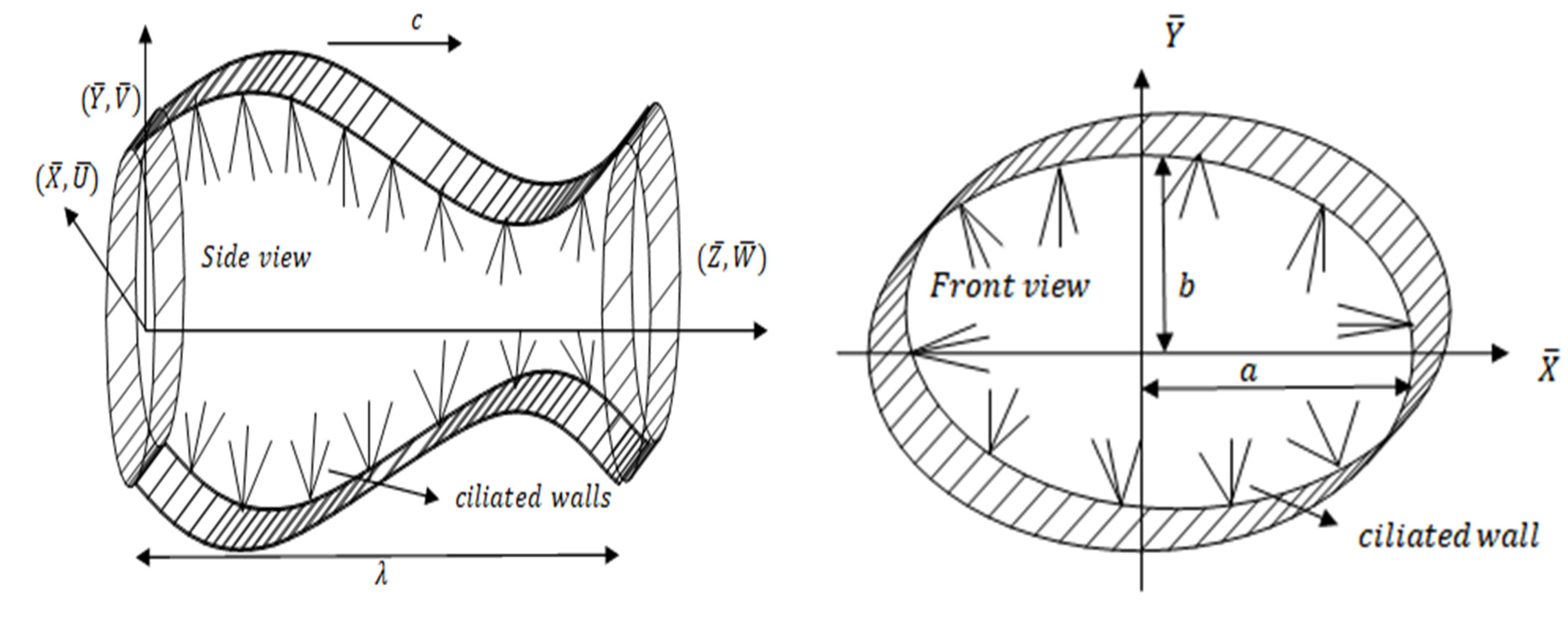
2. Mathematical Model

An innovative model is presented to interpret the convection analysis for a ciliated duct flow and the geometry is presented here, through Figure 1.

The envelope representation of cilia tips is incorporated mathematically by the following equations [23].

$$\begin{gathered} \overline{\mathrm{Y}}={\mathrm{b}}_0+{\mathrm{b}}_0\mathsf{\varphi }\mathrm{Cos}\left(\frac{2\mathsf{\pi }}{\mathsf{\lambda }}\left(\overline{\mathrm{Z}}-\mathrm{c}\overline{\mathrm{t}}\right)\right)=\overline{\mathrm{f}}\left(\overline{\mathrm{Z}},\overline{\mathrm{t}}\right), \\ \overline{\mathrm{Z}}={\overline{\mathrm{Z}}}_0+{\mathrm{b}}_0\mathsf{\varphi }\mathsf{\alpha }\mathrm{Sin}\left(\frac{2\mathsf{\pi }}{\mathsf{\lambda }}\left(\overline{\mathrm{Z}}-\mathrm{c}\overline{\mathrm{t}}\right)\right)=\overline{\mathrm{g}}\left(\overline{\mathrm{Z}},{\overline{\mathrm{Z}}}_0,\overline{\mathrm{t}}\right), \end{gathered}$$

(1)

The velocity (i.e., axial and radial velocity) of cilia tips is provided by these equations

$$\begin{gathered} \overline{\mathrm{W}}={\frac{\partial \overline{\mathrm{Z}}}{\partial \overline{\mathrm{t}}}|}_{{\overline{\mathrm{Z}}}_0}=\frac{\partial \overline{\mathrm{g}}}{\partial \overline{\mathrm{t}}}+\frac{\partial \overline{\mathrm{g}}}{\partial \overline{\mathrm{Z}}}\frac{\partial \overline{\mathrm{Z}}}{\partial \overline{\mathrm{t}}}=\frac{\partial \overline{\mathrm{g}}}{\partial \overline{\mathrm{t}}}+\frac{\partial \overline{\mathrm{g}}}{\partial \overline{\mathrm{Z}}}\overline{\mathrm{W}}, \\ \overline{\mathrm{V}}={\frac{\partial \overline{\mathrm{Y}}}{\partial \overline{\mathrm{t}}}|}_{{\overline{\mathrm{Z}}}_0}=\frac{\partial \overline{\mathrm{f}}}{\partial \overline{\mathrm{t}}}+\frac{\partial \overline{\mathrm{f}}}{\partial \overline{\mathrm{Z}}}\frac{\partial \overline{\mathrm{Z}}}{\partial \overline{\mathrm{t}}}=\frac{\partial \overline{\mathrm{f}}}{\partial \overline{\mathrm{t}}}+\frac{\partial \overline{\mathrm{f}}}{\partial \overline{\mathrm{Z}}}\overline{\mathrm{W}}, \end{gathered}$$

(2)

The combination of Equations (1) and (2) gives

$$\begin{gathered} \overline{\mathrm{W}}=\frac{-\left(\frac{2\mathsf{\pi }}{\mathsf{\lambda }}\right)\left[\mathsf{\varphi }{\mathsf{\alpha }\mathrm{b}}_0\mathrm{c}\mathrm{Cos}\left(\frac{2\mathsf{\pi }}{\mathsf{\lambda }}\left(\overline{\mathrm{Z}}-\mathrm{c}\overline{\mathrm{t}}\right)\right)\right]}{\left[1-\left(\frac{2\mathsf{\pi }}{\mathsf{\lambda }}\right)\left\{\mathsf{\varphi }{\mathsf{\alpha }\mathrm{b}}_0\mathrm{Cos}\left(\frac{2\mathsf{\pi }}{\mathsf{\lambda }}\left(\overline{\mathrm{Z}}-\mathrm{c}\overline{\mathrm{t}}\right)\right)\right\}\right]}, \\ \overline{\mathrm{V}}=\frac{\left(\frac{2\mathsf{\pi }}{\mathsf{\lambda }}\right)\left[\mathsf{\varphi }{\mathrm{b}}_0\mathrm{c}\mathrm{Sin}\left(\frac{2\mathsf{\pi }}{\mathsf{\lambda }}\left(\overline{\mathrm{Z}}-\mathrm{c}\overline{\mathrm{t}}\right)\right)\right]}{\left[1-\left(\frac{2\mathsf{\pi }}{\mathsf{\lambda }}\right)\left\{\mathsf{\varphi }{\mathsf{\alpha }\mathrm{b}}_0\mathrm{Cos}\left(\frac{2\mathsf{\pi }}{\mathsf{\lambda }}\left(\overline{\mathrm{Z}}-\mathrm{c}\overline{\mathrm{t}}\right)\right)\right\}\right]}, \end{gathered}$$

(3)

The two velocities provided here basically differentiate between cilia’s productive and recouping hit. That is $\overline{W}$ and $\overline{V}$, respectively.

The dimensional mathematical equations that model this problem for an incompressible Jeffrey fluid are provided as [24]

$${\overline{U}}_x+{\overline{V}}_y+{\overline{W}}_z=0,$$

(4)

$$\mathsf{\rho }\left({\overline{U}}_t+\overline{\mathrm{U}}{\overline{U}}_x+\overline{\mathrm{V}}{\overline{U}}_y+\overline{\mathrm{W}}{\overline{U}}_z\right)=-{\overline{P}}_x+{(\overline{\mathrm{S}}}_{\overline{\mathrm{X}}\overline{\mathrm{X}}}{)}_x+{\left({\overline{\mathrm{S}}}_{\overline{\mathrm{Y}}\overline{\mathrm{X}}}\right)}_y+{({\overline{\mathrm{S}}}_{\overline{\mathrm{Z}}\overline{\mathrm{X}}})}_z,$$

(5)

$$\mathsf{\rho }\left({\overline{V}}_t+\overline{\mathrm{U}}{\overline{V}}_x+\overline{\mathrm{V}}{\overline{V}}_y+\overline{\mathrm{W}}{\overline{V}}_z\right)=-{\overline{P}}_y+{(\overline{\mathrm{S}}}_{\overline{\mathrm{X}}\overline{Y}}{)}_x+{\left({\overline{\mathrm{S}}}_{\overline{\mathrm{Y}}\overline{Y}}\right)}_y+{({\overline{\mathrm{S}}}_{\overline{\mathrm{Z}}\overline{Y}})}_z,$$

(6)

$$\mathsf{\rho }\left({\overline{W}}_t+\overline{\mathrm{U}}{\overline{W}}_x+\overline{\mathrm{V}}{\overline{W}}_y+\overline{\mathrm{W}}{\overline{W}}_z\right)=-{\overline{P}}_z+{(\overline{\mathrm{S}}}_{\overline{\mathrm{X}}\overline{Z}}{)}_x+{\left({\overline{\mathrm{S}}}_{\overline{\mathrm{Y}}\overline{Z}}\right)}_y+{({\overline{\mathrm{S}}}_{\overline{\mathrm{Z}}\overline{Z}})}_z,$$

(7)

$$\begin{gathered} {\mathsf{\rho }\mathrm{C}}_{\mathrm{p}}\left({\overline{T}}_t+\overline{\mathrm{U}}{\overline{T}}_x+\overline{\mathrm{V}}{\overline{T}}_y+\overline{\mathrm{W}}{\overline{T}}_z\right) \\ =\mathrm{k}\left({\overline{T}}_{xx}+{\overline{T}}_{yy}+{\overline{T}}_{zz}\right)+{\overline{\mathrm{S}}}_{\overline{\mathrm{X}}\overline{\mathrm{X}}}{\overline{U}}_x+{\overline{\mathrm{S}}}_{\overline{\mathrm{X}}\overline{\mathrm{Y}}}{\overline{U}}_y+{\overline{\mathrm{S}}}_{\overline{\mathrm{X}}\overline{\mathrm{Z}}}{\overline{U}}_z+{\overline{\mathrm{S}}}_{\overline{\mathrm{Y}}\overline{\mathrm{X}}}{\overline{V}}_x+{\overline{\mathrm{S}}}_{\overline{\mathrm{Y}}\overline{\mathrm{Y}}}{\overline{V}}_y+{\overline{\mathrm{S}}}_{\overline{\mathrm{Y}}\overline{\mathrm{Z}}}{\overline{V}}_z \\ +{\overline{\mathrm{S}}}_{\overline{\mathrm{Z}}\overline{\mathrm{X}}}{\overline{W}}_x+{\overline{\mathrm{S}}}_{\overline{\mathrm{Z}}\overline{\mathrm{Y}}}{\overline{W}}_y+{\overline{\mathrm{S}}}_{\overline{\mathrm{Z}}\overline{\mathrm{Z}}}{\overline{W}}_z, \end{gathered}$$

(8)

The mathematical description of boundary conditions is conveyed in dimensional form, as follows

$$\begin{gathered} \overline{\mathrm{W}}=\frac{-\left(\frac{2\mathsf{\pi }}{\mathsf{\lambda }}\right)\left[\mathsf{\varphi }{\mathsf{\alpha }\mathrm{b}}_0\mathrm{c}\mathrm{Cos}\left(\frac{2\mathsf{\pi }}{\mathsf{\lambda }}\left(\overline{\mathrm{Z}}-\mathrm{c}\overline{\mathrm{t}}\right)\right)\right]}{\left[1-\left(\frac{2\mathsf{\pi }}{\mathsf{\lambda }}\right)\left\{\mathsf{\varphi }{\mathsf{\alpha }\mathrm{b}}_0\mathrm{Cos}\left(\frac{2\mathsf{\pi }}{\mathsf{\lambda }}\left(\overline{\mathrm{Z}}-\mathrm{c}\overline{\mathrm{t}}\right)\right)\right\}\right]}\mathrm{for}\frac{{\overline{\mathrm{x}}}^2}{{\overline{\mathrm{a}}}^2}+\frac{{\overline{\mathrm{y}}}^2}{{\overline{\mathrm{b}}}^2}=1. \\ \overline{\mathrm{T}}={\overline{\mathrm{T}}}_{\mathrm{w}}\mathrm{for}\frac{{\overline{\mathrm{x}}}^2}{{\overline{\mathrm{a}}}^2}+\frac{{\overline{\mathrm{y}}}^2}{{\overline{\mathrm{b}}}^2}=1. \end{gathered}$$

(9)

The non-Newtonian Jeffrey fluid is incorporated in the present analysis by using the following relation of extra stress tensor [25,26,27].

$$\overline{\mathrm{S}}=\frac{\mathsf{\mu }}{1+{\mathsf{\lambda }}_1}\left(\dot{\mathsf{\gamma }}+{\mathsf{\lambda }}_2\ddot{\mathsf{\gamma }}\right),$$

(10)

The mathematical relation between the two frames is provided by

$$\overline{\mathrm{x}}=\overline{\mathrm{X}},\overline{\mathrm{y}}=\overline{\mathrm{Y}},\overline{\mathrm{z}}=\overline{\mathrm{Z}}-\mathrm{c}\overline{\mathrm{t}},\overline{\mathrm{p}}=\overline{\mathrm{P}},\overline{\mathrm{u}}=\overline{\mathrm{U}},\overline{\mathrm{v}}=\overline{\mathrm{V}},\overline{\mathrm{w}}=\overline{\mathrm{W}}-\mathrm{c},$$

(11)

The functional dimensionless quantities used here are

$$\begin{gathered} \mathrm{x}=\frac{\overline{\mathrm{x}}}{{\mathrm{D}}_{\mathrm{h}}},\mathrm{t}=\frac{\mathrm{c}\overline{\mathrm{t}}}{\mathsf{\lambda }},\mathrm{w}=\frac{\overline{\mathrm{w}}}{\mathrm{c}},\mathrm{z}=\frac{\overline{\mathrm{z}}}{\mathsf{\lambda }},\mathrm{p}=\frac{{\mathrm{D}}_{\mathrm{h}}^2\overline{\mathrm{p}}}{\mathsf{\mu }\mathsf{\lambda }\mathrm{c}},\mathrm{y}=\frac{\overline{\mathrm{y}}}{{\mathrm{D}}_{\mathrm{h}}},\mathsf{\theta }=\frac{\overline{\mathrm{T}}-{\overline{\mathrm{T}}}_{\mathrm{w}}}{{\overline{\mathrm{T}}}_{\mathrm{b}}-{\overline{\mathrm{T}}}_{\mathrm{w}}},\mathsf{\delta }=\frac{{\mathrm{b}}_0}{{\mathrm{a}}_0}, \\ \mathsf{\varphi }=\frac{\mathrm{d}}{{\mathrm{b}}_0},{\mathrm{B}}_{\mathrm{r}}=\frac{{\mathsf{\mu }\mathrm{c}}^2}{\mathrm{k}\left({\overline{\mathrm{T}}}_{\mathrm{b}}-{\overline{\mathrm{T}}}_{\mathrm{w}}\right)},\mathrm{u}=\frac{\mathsf{\lambda }\overline{\mathrm{u}}}{{\mathrm{D}}_{\mathrm{h}}\mathrm{c}},\mathrm{v}=\frac{\mathsf{\lambda }\overline{\mathrm{v}}}{{\mathrm{D}}_{\mathrm{h}}\mathrm{c}},\mathrm{S}=\frac{{\mathrm{D}}_{\mathrm{h}}\overline{\mathrm{S}}}{\mathrm{c}\mathsf{\mu }},\mathrm{a}=\frac{\overline{\mathrm{a}}}{{\mathrm{D}}_{\mathrm{h}}},\mathrm{b}=\frac{\overline{\mathrm{b}}}{{\mathrm{D}}_{\mathrm{h}}},\mathsf{\beta }=\frac{{\mathrm{b}}_0}{\mathsf{\lambda }}, \end{gathered}$$

(12)

The ellipse has the following hydraulic diameter

$${\mathrm{D}}_{\mathrm{h}}=\frac{{\mathsf{\pi }\mathrm{b}}_0}{\mathrm{E}\left(\mathrm{e}\right)},$$

(13)

Now, $e=\sqrt{1-{\delta }^2}$, presents $E\left(e\right)$ i.e., eccentricity, provided as [28].

$$\mathrm{E}\left(\mathrm{e}\right)=\underset{0}{\overset{\raisebox{1ex}{$\mathsf{\pi }$}\!\left/ \!\raisebox{-1ex}{$2$}\right.}{{\displaystyle \int }}}\sqrt{1-{\mathrm{e}}^2{\mathrm{Sin}}^2{\mathsf{\alpha }}_1}{\mathrm{d}\mathsf{\alpha }}_1,$$

(14)

The above formulated computational problem is transformed into its non-dimensional mathematical form and the final simplified form is achieved by using the approximation ($\lambda \to \infty$).

$$\frac{\partial \mathrm{p}}{\partial \mathrm{x}}=0,$$

(15)

$$\frac{\partial \mathrm{p}}{\partial \mathrm{y}}=0,$$

(16)

$$\frac{\mathrm{dp}}{\mathrm{dz}}=\left(\frac{1}{1+{\mathsf{\lambda }}_1}\right)\left(\frac{{\partial }^2\mathrm{w}}{\partial {\mathrm{x}}^2}+\frac{{\partial }^2\mathrm{w}}{\partial {\mathrm{y}}^2}\right),$$

(17)

$$\frac{{\partial }^2\mathsf{\theta }}{\partial {\mathrm{x}}^2}+\frac{{\partial }^2\mathsf{\theta }}{\partial {\mathrm{y}}^2}+{\mathrm{B}}_{\mathrm{r}}\left(\frac{1}{1+{\mathsf{\lambda }}_1}\right)\left[{\left(\frac{\partial \mathrm{w}}{\partial \mathrm{x}}\right)}^2+{\left(\frac{\partial \mathrm{w}}{\partial \mathrm{y}}\right)}^2\right]=0,$$

(18)

The associated conditions on boundaries are

$$\mathrm{w}=-1-\frac{2\mathsf{\pi }\mathsf{\varphi }\mathsf{\alpha }\mathsf{\beta }\mathrm{Cos}\left(2\mathsf{\pi }\mathrm{z}\right)}{1-2\mathsf{\pi }\mathsf{\varphi }\mathsf{\alpha }\mathsf{\beta }\mathrm{Cos}\left(2\mathsf{\pi }\mathrm{z}\right)},\mathrm{for}\frac{{\mathrm{x}}^2}{{\mathrm{a}}^2}+\frac{{\mathrm{y}}^2}{{\mathrm{b}}^2}=1.$$

(19)

$$\mathsf{\theta }=0,\mathrm{for}\frac{{\mathrm{x}}^2}{{\mathrm{a}}^2}+\frac{{\mathrm{y}}^2}{{\mathrm{b}}^2}=1,$$

(20)

Moreover, $\mathrm{a}=\frac{\mathrm{E}\left(\mathrm{e}\right)}{\mathsf{\pi }}\left[\frac{1}{\mathsf{\delta }}+\mathsf{\varphi }\mathrm{Sin}\left(2\mathsf{\pi }\mathrm{z}\right)\right],$ and $\mathrm{b}=\frac{\mathrm{E}\left(\mathrm{e}\right)}{\mathsf{\pi }}\left[1+\mathsf{\varphi }\mathrm{Sin}\left(2\mathsf{\pi }\mathrm{z}\right)\right].$

3. Exact Solution

Consider a solution of velocity in the form of the following polynomial expression [29]

$$w\left(x,y\right)=K_1{x}^4+K_2{y}^4+K_3{x}^2{y}^2+K_4{x}^2+K_5{y}^2+K_6,$$

(21)

The solution of velocity can be written in this polynomial form, since the following polynomial, when used in momentum equation and corresponding boundary conditions, gives an exact solution of flow profile that exactly satisfies the equation and boundary conditions.

Substituting Equation (21) in Equation (17) and making comparison of $x^2, y^2, x^0, y^0$ coefficients on both sides of the Equation, we utilize the three Equations

$$12K_1+2K_3=0,$$

(i)

$$2K_3+12K_2=0,$$

(ii)

$$2K_4+2K_5=\frac{\mathrm{dp}}{\mathrm{dz}}\left(1+{\mathsf{\lambda }}_1\right),$$

(iii)

Also, we avail three more Equations by using Equation (21) in (19) and coefficients balancing of $x^4, x^2, x^0$ gives

$$K_1{\mathrm{a}}^4+K_2{\mathrm{b}}^4-K_3{\mathrm{a}}^2{\mathrm{b}}^2=0,$$

(iv)

$$-2K_2{\mathrm{b}}^4+K_3{\mathrm{a}}^2{\mathrm{b}}^2+K_4{\mathrm{a}}^2-K_5{\mathrm{b}}^2=0,$$

(v)

$$K_2{\mathrm{b}}^4+K_5{\mathrm{b}}^2+K_6=-1-\frac{2\mathsf{\pi }\mathsf{\varphi }\mathsf{\alpha }\mathsf{\beta }\mathrm{Cos}\left(2\mathsf{\pi }\mathrm{z}\right)}{1-2\mathsf{\pi }\mathsf{\varphi }\mathsf{\alpha }\mathsf{\beta }\mathrm{Cos}\left(2\mathsf{\pi }\mathrm{z}\right)},$$

(vi)

We can solve these six Equations (i)–(vi) and have

$$\begin{gathered} K_1=0,K_2=0,K_3=0,K_4=\frac{{\mathrm{b}}^2\frac{\mathrm{dp}}{\mathrm{dz}}\left(1+{\mathsf{\lambda }}_1\right)}{2\left({\mathrm{a}}^2+{\mathrm{b}}^2\right)}, \\ {K}_5=\frac{{\mathrm{a}}^2\frac{\mathrm{dp}}{\mathrm{dz}}\left(1+{\mathsf{\lambda }}_1\right)}{2\left({\mathrm{a}}^2+{\mathrm{b}}^2\right)},K_6=-\frac{{\mathrm{a}}^2{\mathrm{b}}^2\frac{\mathrm{dp}}{\mathrm{dz}}\left(1+{\mathsf{\lambda }}_1\right)}{2\left({\mathrm{a}}^2+{\mathrm{b}}^2\right)}+\frac{1}{2\mathsf{\pi }\mathsf{\varphi }\mathsf{\alpha }\mathsf{\beta }\mathrm{Cos}\left(2\mathsf{\pi }\mathrm{z}\right)-1}, \end{gathered}$$

The values of these constants are utilized in Equation (21) and this provides an exact velocity solution given as

$$\mathrm{w}\left(\mathrm{x},\mathrm{y}\right)=-1-\frac{2\mathsf{\pi }\mathsf{\varphi }\mathsf{\alpha }\mathsf{\beta }\mathrm{Cos}\left(2\mathsf{\pi }\mathrm{z}\right)}{1-2\mathsf{\pi }\mathsf{\varphi }\mathsf{\alpha }\mathsf{\beta }\mathrm{Cos}\left(2\mathsf{\pi }\mathrm{z}\right)}+\frac{1}{2}\frac{{\mathrm{a}}^2{\mathrm{b}}^2\left(1+{\mathsf{\lambda }}_1\right)}{({\mathrm{a}}^2+{\mathrm{b}}^2)}\frac{\mathrm{dp}}{\mathrm{dz}}\left(\frac{{\mathrm{x}}^2}{{\mathrm{a}}^2}+\frac{{\mathrm{y}}^2}{{\mathrm{b}}^2}-1\right),$$

(22)

The exact value of $q\left(z\right)$ is computed by integration of (22)

$$\mathrm{q}\left(\mathrm{z}\right)=-\frac{{\mathrm{a}}^3{\mathrm{b}}^3\frac{\mathrm{dp}}{\mathrm{dz}}\mathsf{\pi }\left(1+{\mathsf{\lambda }}_1\right)}{4\left({\mathrm{a}}^2+{\mathrm{b}}^2\right)}+\frac{\mathrm{ab}\mathsf{\pi }}{-1+2\mathsf{\pi }\mathsf{\varphi }\mathsf{\alpha }\mathsf{\beta }\mathrm{Cos}\left(2\mathsf{\pi }\mathrm{z}\right)},$$

(23)

From Equation (23), $\frac{dp}{dz}$ is computed as

$$\frac{\mathrm{dp}}{\mathrm{dz}}=\frac{4\left({\mathrm{a}}^2+{\mathrm{b}}^2\right)\left[-{{\displaystyle \int }}_0^1\mathrm{abdz}+\mathrm{ab}\mathsf{\pi }+\mathrm{Q}+2\mathsf{\pi }\left({{\displaystyle \int }}_0^1\mathrm{abdz}-\mathrm{Q}\right)\mathsf{\alpha }\mathsf{\beta }\mathsf{\varphi }\mathrm{Cos}\left(2\mathsf{\pi }\mathrm{z}\right)\right]}{{\mathrm{a}}^3{\mathrm{b}}^3\mathsf{\pi }\left(1+{\mathsf{\lambda }}_1\right)\left(-1+2\mathsf{\pi }\mathsf{\varphi }\mathsf{\alpha }\mathsf{\beta }\mathrm{Cos}\left(2\mathsf{\pi }\mathrm{z}\right)\right)},$$

(24)

The mathematical relation that is used to evaluate the pressure rise for a single wavelength is given as

$$\mathsf{\Delta }\mathrm{P}=\underset{0}{\overset{1}{{\displaystyle \int }}}\frac{\partial \mathrm{p}}{\partial \mathrm{z}}\mathrm{dz},$$

(25)

The exact mathematical result of temperature is computed as

$$\theta \left(x,y\right)=\frac{-B_r{\left(\frac{dp}{dz}\right)}^2{a}^2{b}^2\left(\frac{x^2}{a^2}+\frac{y^2}{b^2}-1\right)\left[b^6{x}^2+a^2{b}^4\left(b^2+6x^2-y^2\right)+a^6\left(b^2+y^2\right)+a^4{b}^2\left(4b^2-x^2+6y^2\right)\right]\left(1+{\lambda }_1\right)}{12{\left(a^2+b^2\right)}^2\left(a^4+6a^2{b}^2+b^4\right)},$$

(26)

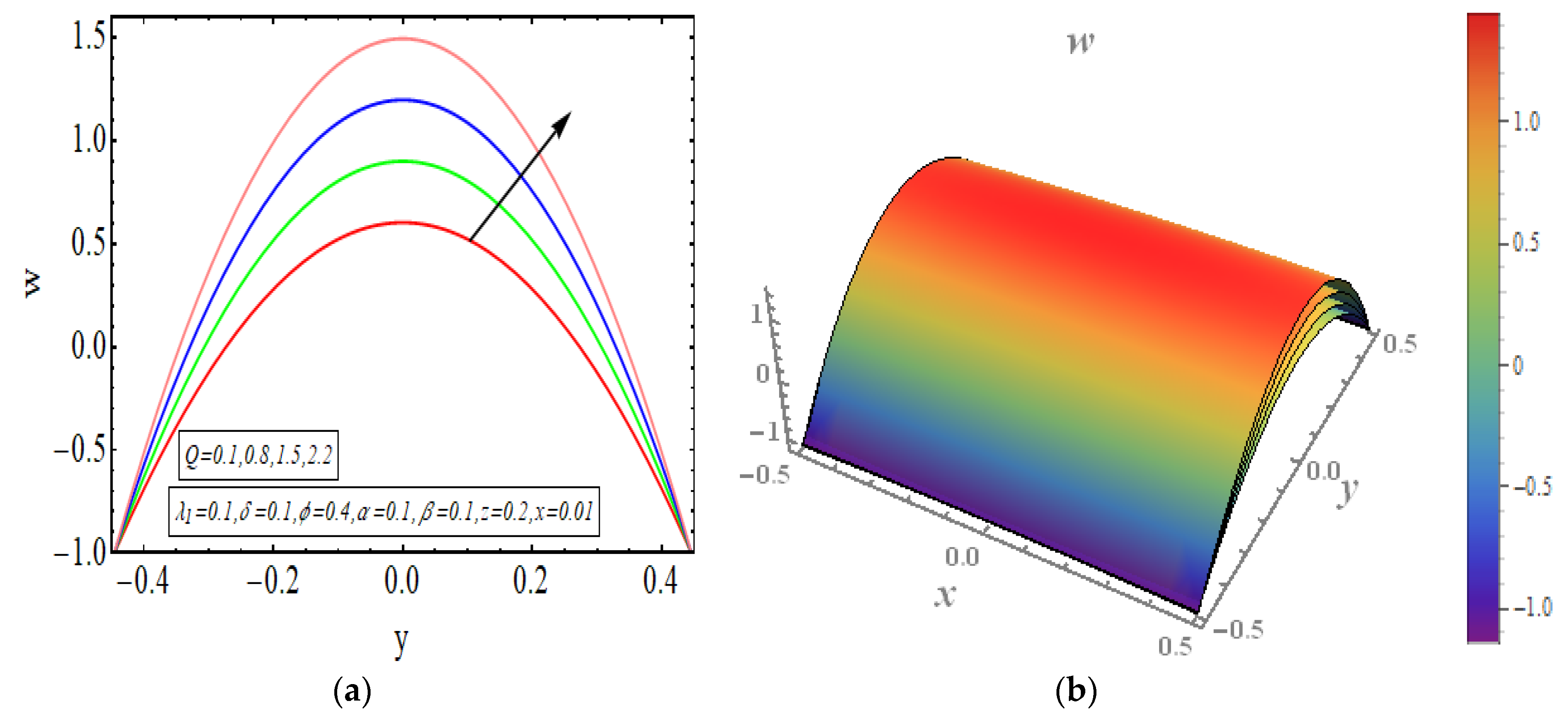
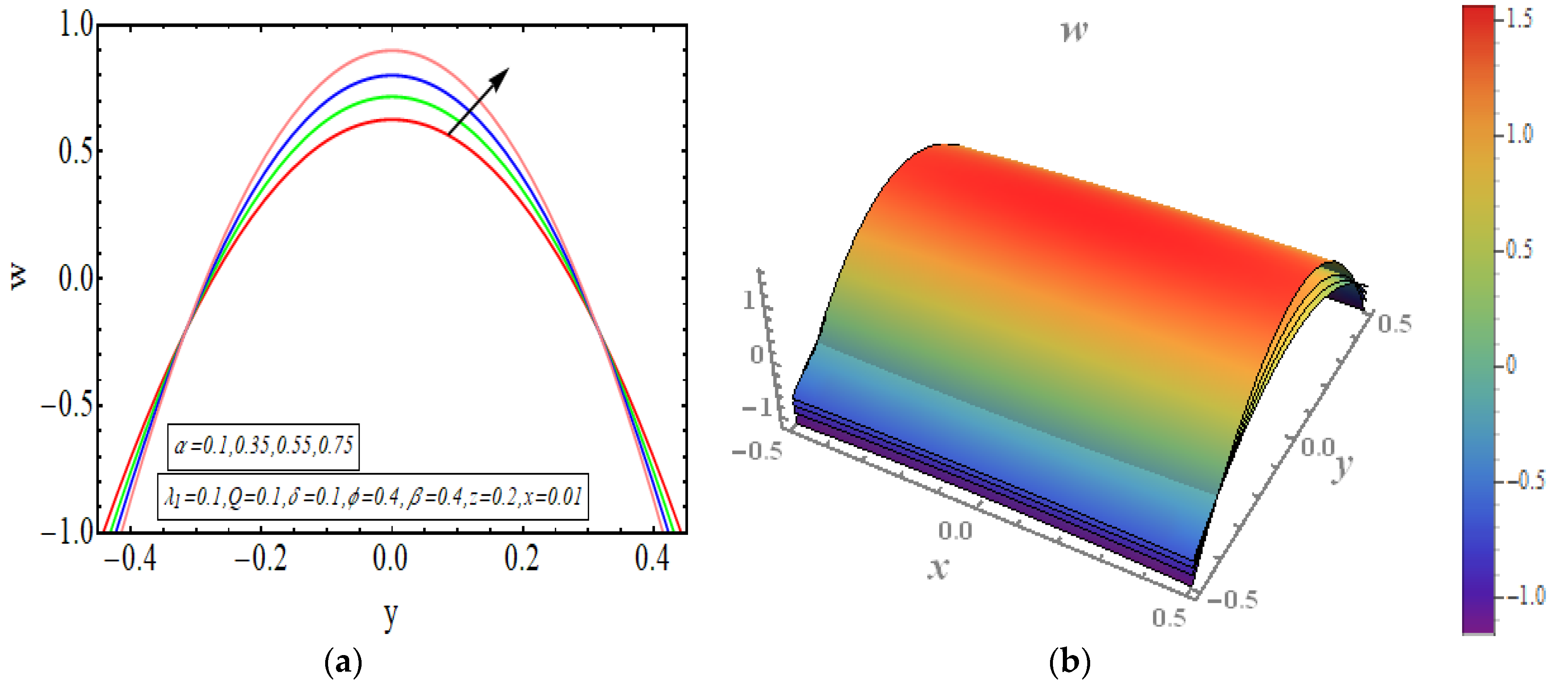
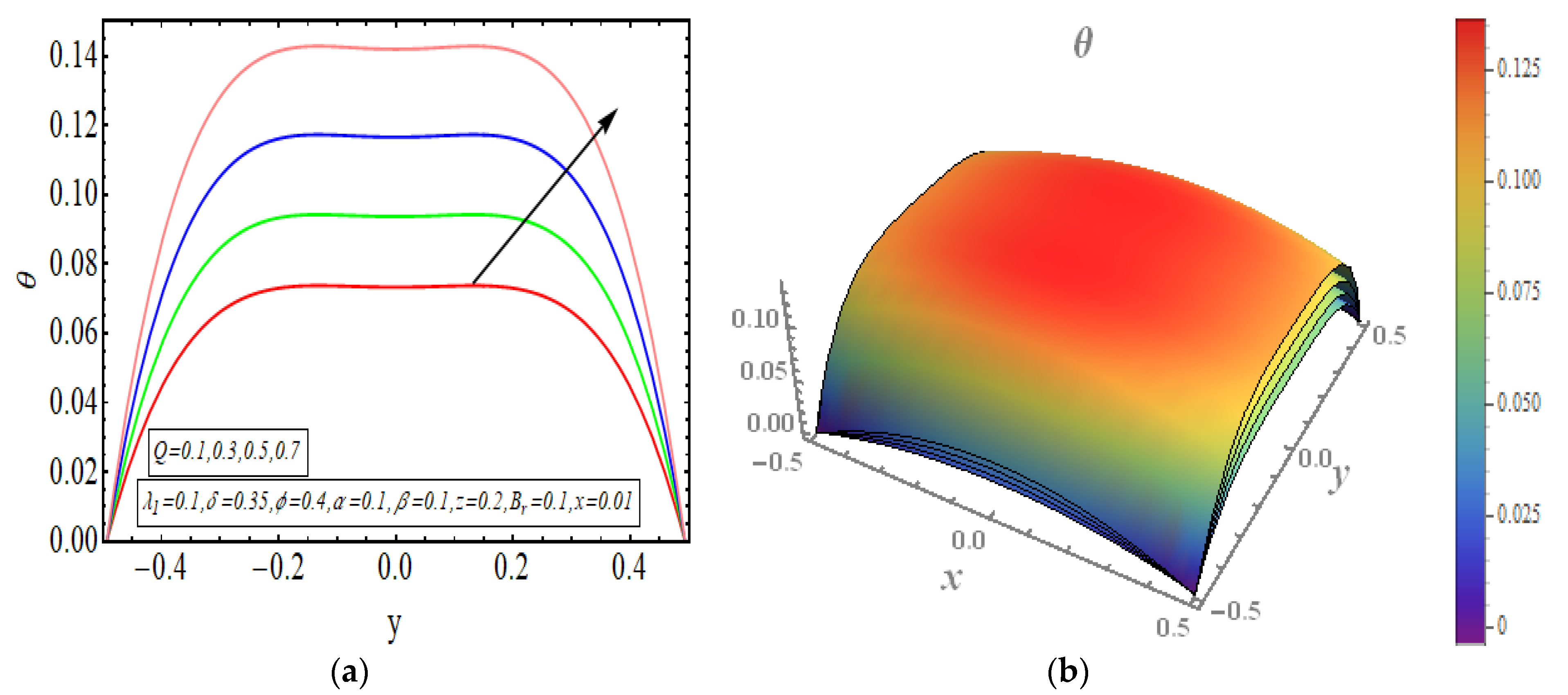
4. Results and Discussion

The graphical outcomes presented in this section provide comprehensive detail about the distinct characteristics of peristaltic flow in this ciliated duct with elliptic cross section. Figure 2, Figure 3 and Figure 4 provide the graphical outcomes of velocity, subject to the impact of distinct physical parameters. These graphs include the 2D and 3D plots of velocity profile. An increase is observed in velocity as $Q$ increases, revealed by Figure 2a. Figure 2b provides the 3D graphical plot of velocity, which reveals flow dependency on x in addition to y. The velocity has inflative value in the middle of the conduit and a parabolic velocity profile is noted. Figure 3a,b reveal an increment in the flow profile for increasing $\beta$. The enhancing $\beta$ results in an increased flow profile in the middle of the duct but it declines with increasing $\beta$ near the ciliated boundaries. An axial symmetry and parabolic velocity profile is observed. Figure 4a,b provide the 2D and 3D velocity plots for enhancing $\alpha$. An increase in the velocity is seen for incrementing $\alpha$. The flow profile attains high magnitude in the central region of the conduit but it shows an opposite behaviour near the ciliated boundaries with an increasing value of $\alpha$. The increasing behaviour of velocity at the centre changes to a declining one near the ciliated walls. All the velocity graphs reveal that the flow behaviour is axially symmetric and a parabolic velocity profile is observed. Figure 5, Figure 6, Figure 7, Figure 8 and Figure 9 provide the graphical solutions of temperature profile and its dependence on various parameters. Figure 5a,b provide the temperature plots for various numerical values of $Q$. Temperature attains high values for increasing $Q$. An axially symmetrical temperature behaviour is also observed in these temperature graphs. The convection rate is highest at the middle and minimum, near the ciliated boundaries. Figure 6a,b reveal the numerical solution of temperature for the uprising value of ${\lambda }_1$. A decline in the temperature profile is observed for increasing values of ${\lambda }_1$. If we set ${\lambda }_1=0$ then the problem is simply a Newtonian flow problem. The increase in the value of ${\lambda }_1$ changes the problem to a non-Newtonian flow problem. It reveals that the temperature reduces if the problem is transformed from analysis of a Newtonian to non-Newtonian flow problem. Figure 7a,b give the temperature solution for rising $\beta$. A rise in the temperature profile is observed for upsurging $\beta$. The convection is highest at the middle section of the conduit and then starts reducing on the way to the ciliated boundaries of the duct. Figure 8a,b provide the 2D and 3D plot of temperature for upsurging $B_r$. The temperature rapidly increases for an increasing value of $B_r$. An axially balanced temperature profile is revealed for the incrementing value of $B_r$. The highest temperature in the middle of the conduit starts declining towards the ciliated boundaries and eventually becomes zero. Figure 9a,b depict the 2D and 3D plot of heat flux for distinct numerical entities of $\alpha$. An increase in the convection rate is noted for upsurging $\alpha$. The maximum temperature is noted at the centre and zero at the ciliated walls. In Figure 10a–d, $\frac{dp}{dz}$ is plotted against the axial coordinate and its dependence on various parameters is noted. Figure 10a depicts that $\frac{dp}{dz}$ gains higher values with increasing the value of $\delta$. Figure 10b reveals an increment in $\frac{dp}{dz}$ for uprising ${\mathsf{\lambda }}_1$. Figure 10c shows that $\frac{dp}{dz}$ increases in the crest region of the peristaltic wave but it diminishes in the trough region of the peristaltic wave for the incrementing value of $\varphi$. Figure 10d depicts a decline in $\frac{dp}{dz}$ for increasing $Q$. In Figure 11a–c $\Delta P$ against $Q$ is drawn for distinct uprising values of the physical parameters. Figure 11a depicts the outcome of $\Delta P$ against $Q$ for increasing $\delta$. A rise in $\mathsf{\Delta }P$ is revealed in the section $\mathsf{\Delta }P>0$ but a decline is noted in the section $\mathsf{\Delta }P<0$. Figure 11b conveys the numerical result of $\mathsf{\Delta }P$ against $Q$ for enhancing ${\lambda }_1$. A declining numerical value of $\mathsf{\Delta }P$ is noted in the segment $\mathsf{\Delta }P>0$ but an increment is observed in segment $\mathsf{\Delta }P<0$. Figure 11c reveals that $\mathsf{\Delta }P$ against $Q$ gains higher value in the region $\mathsf{\Delta }P>0$ but its value declines in the region $\mathsf{\Delta }P<0$ for increasing $\varphi .$ The streamline plots are also added for incrementing $Q$, displayed in Figure 12a–d. The trapped closed contours show an increase in size with incrementing $Q$. The graphical picture of flow is conveyed through these streamline outcomes.

5. Conclusions

The current research was carried out to analyse the convection analysis of heated Jeffrey fluid in a conduit having elliptic domain and ciliated boundaries. The key outcomes are given below. The velocity gains its highest magnitude in the middle region of the conduit and a parabolic velocity profile is seen. The velocity gains magnitude with the increasing value of $\beta$ in the middle of the duct but it declines with increasing $\beta$ near the ciliated boundaries. An axial symmetry and parabolic velocity profile is observed. An axially symmetrical temperature behaviour is also observed in these temperature graphs. The temperature has high magnitude in the middle and low sections near the ciliated boundaries. A decline in the temperature profile is observed for increasing values of ${\mathsf{\lambda }}_1$. If we set ${\lambda }_1=0$ then the problem is simply a Newtonian flow problem. The increase in the value of ${\lambda }_1$ changes the problem to a non-Newtonian flow problem. It is observed that the temperature reduces if the problem is transformed from Newtonian analysis to a non-Newtonian one. The temperature rapidly increases for the increasing value of $B_r$. The trapped close contours show an increase in size for rising $Q$.

References

1. Abdel-Wahed, R.M.; Attia, A.E.; Hifni, M.A. Experiments on laminar flow and heat transfer in an elliptical duct. Int. J. Heat Mass Transf. 1984, 27, 2397–2413. [Google Scholar] [CrossRef]
2. Maia, C.R.M.; Aparecido, J.B.; Milanez, L.F. Heat transfer in laminar flow of non-Newtonian fluids in ducts of elliptical section. Int. J. Therm. Sci. 2006, 45, 1066–1072. [Google Scholar] [CrossRef]
3. Ragueb, H.; Mansouri, K. An analytical study of the periodic laminar forced convection of non-Newtonian nanofluid flow inside an elliptical duct. Int. J. Heat Mass Transf. 2018, 127, 469–483. [Google Scholar] [CrossRef]
4. Barton, C.; Raynor, S. Peristaltic flow in tubes. Bull. Math. Biophys. 1968, 30, 663–680. [Google Scholar] [CrossRef] [PubMed]
5. Böhme, G.; Friedrich, R. Peristaltic flow of viscoelastic liquids. J. Fluid Mech. 1983, 128, 109–122. [Google Scholar] [CrossRef]
6. Nadeem, S.; Akbar, N.S. Influence of heat transfer on a peristaltic flow of Johnson Segalman fluid in a non uniform tube. Int. Commun. Heat Mass Transf. 2009, 36, 1050–1059. [Google Scholar] [CrossRef]
7. Akbar, N.S.; Nadeem, S.; Hayat, T.; Hendi, A.A. Peristaltic flow of a nanofluid in a non-uniform tube. Heat Mass Transf. 2012, 48, 451–459. [Google Scholar] [CrossRef]
8. Akbar, N.S.; Nadeem, S. Peristaltic flow of a Phan-Thien-Tanner nanofluid in a diverging tube. Heat Transf.—Asian Res. 2012, 41, 10–22. [Google Scholar] [CrossRef]
9. Akbar, N.S.; Nadeem, S. Combined effects of heat and chemical reactions on the peristaltic flow of Carreau fluid model in a diverging tube. Int. J. Numer. Methods Fluids 2011, 67, 1818–1832. [Google Scholar] [CrossRef]
10. Nadeem, S.; Maraj, E.N. The mathematical analysis for peristaltic flow of hyperbolic tangent fluid in a curved channel. Commun. Theor. Phys. 2013, 59, 729. [Google Scholar] [CrossRef]
11. Nadeem, S.; Shahzadi, I. Mathematical analysis for peristaltic flow of two phase nanofluid in a curved channel. Commun. Theor. Phys. 2015, 64, 547. [Google Scholar] [CrossRef]
12. Nadeem, S.; Akram, S. Peristaltic flow of a Jeffrey fluid in a rectangular duct. Nonlinear Anal. Real World Appl. 2010, 11, 4238–4247. [Google Scholar] [CrossRef]
13. Ellahi, R.; Riaz, A.; Nadeem, S. Three dimensional peristaltic flow of Williamson fluid in a rectangular duct. Indian J. Phys. 2013, 87, 1275–1281. [Google Scholar] [CrossRef]
14. Akram, S.; Saleem, N. Analysis of Heating Effects and Different Wave Forms on Peristaltic Flow of Carreau Fluid in Rectangular Duct. Adv. Math. Phys. 2020, 2020, 8294318. [Google Scholar] [CrossRef]
15. Saleem, A.; Akhtar, S.; Nadeem, S.; Alharbi, F.M.; Ghalambaz, M.; Issakhov, A. Mathematical computations for Peristaltic flow of heated non-Newtonian fluid inside a sinusoidal elliptic duct. Phys. Scr. 2020, 95, 105009. [Google Scholar] [CrossRef]
16. Akbar, N.S.; Butt, A.W. Heat transfer analysis of viscoelastic fluid flow due to metachronal wave of cilia. Int. J. Biomath. 2014, 7, 1450066. [Google Scholar] [CrossRef]
17. Akbar, N.S.; Khan, Z.H. Influence of magnetic field for metachoronical beating of cilia for nanofluid with Newtonian heating. J. Magn. Magn. Mater. 2015, 381, 235–242. [Google Scholar] [CrossRef]
18. Saleem, A.; Akhtar, S.; Alharbi, F.M.; Nadeem, S.; Ghalambaz, M.; Issakhov, A. Physical aspects of peristaltic flow of hybrid nano fluid inside a curved tube having ciliated wall. Results Phys. 2020, 19, 103431. [Google Scholar] [CrossRef]
19. Butt, A.W.; Akbar, N.S.; Mir, N.A. Heat transfer analysis of peristaltic flow of a Phan-Thien–Tanner fluid model due to metachronal wave of cilia. Biomech. Model. Mechanobiol. 2020, 19, 1925–1933. [Google Scholar] [CrossRef]
20. Pavlovsky, V.A. On theoretical description of weak aqueous solutions of polymers. In Doklady Akademii Nauk; Russian Academy of Sciences: Moscow, Russia, 1971; Volume 200, pp. 809–812. [Google Scholar]
21. Baranovskii, E.S. Flows of a polymer fluid in domain with impermeable boundaries. Comput. Math. Math. Phys. 2014, 54, 1589–1596. [Google Scholar] [CrossRef]
22. Baranovskii, E.S. Global solutions for a model of polymeric flows with wall slip. Math. Methods Appl. Sci. 2017, 40, 5035–5043. [Google Scholar] [CrossRef]
23. Sadaf, H.; Nadeem, S. Fluid flow analysis of cilia beating in a curved channel in the presence of magnetic field and heat transfer. Can. J. Phys. 2020, 98, 191–197. [Google Scholar] [CrossRef]
24. McCash, L.B.; Nadeem, S.; Akhtar, S.; Saleem, A.; Saleem, S.; Issakhov, A. Novel idea about the peristaltic flow of heated Newtonian fluid in elliptic duct having ciliated walls. Alex. Eng. J. 2022, 61, 2697–2707. [Google Scholar] [CrossRef]
25. Nadeem, S.; Akbar, N.S. Peristaltic flow of a Jeffrey fluid with variable viscosity in an asymmetric channel. Z. Für Nat. A 2009, 64, 713–722. [Google Scholar] [CrossRef]
26. Bhatti, M.M.; Jun, S.; Khalique, C.M.; Shahid, A.; Fasheng, L.; Mohamed, M.S. Lie group analysis and robust computational approach to examine mass transport process using Jeffrey fluid model. Appl. Math. Comput. 2022, 421, 126936. [Google Scholar] [CrossRef]
27. Mehboob, H.; Maqbool, K.; Ullah, H.; Siddiqui, A.M. Computational analysis of an axisymmetric flow of Jeffrey fluid in a permeable micro channel. Appl. Math. Comput. 2022, 418, 126826. [Google Scholar] [CrossRef]
28. Yang, Z.H.; Chu, Y.M.; Zhang, W. Monotonicity of the ratio for the complete elliptic integral and Stolarsky mean. J. Inequalities Appl. 2016, 2016, 176. [Google Scholar] [CrossRef] [Green Version]
29. Hayman, W.K.; Shanidze, Z.G. Polynomial solutions of partial differential equations. Methods Appl. Anal. 1999, 6, 97–108. [Google Scholar] [CrossRef] [Green Version]
Figure 1. Side and front view geometrical model.
Applsci 12 05065 g001
Figure 2. (a) Velocity for Q (2D). (b) Velocity for Q (3D).
Applsci 12 05065 g002
Figure 3. (a) Velocity for β (2D). (b) Velocity for (3D).
Applsci 12 05065 g003
Figure 4. (a) Velocity for α (2D). (b) Velocity for α (3D).
Applsci 12 05065 g004
Figure 5. (a) Temperature for Q (2D). (b) Temperature for Q (3D).
Applsci 12 05065 g005
Figure 6. (a) Temperature for λ 1 (2D). (b) Temperature for λ 1 (3D).
Applsci 12 05065 g006
Figure 7. (a) Temperature for β (2D). (b) Temperature for β (3D).
Applsci 12 05065 g007
Figure 8. (a) Temperature for B r (2D). (b) Temperature for B r (3D).
Applsci 12 05065 g008
Figure 9. (a) Temperature for α (2D). (b) Temperature for α (3D).
Applsci 12 05065 g009
Figure 10. (a) d p d z against z-axis for δ . (b) d p d z against z-axis for λ 1 . (c) d p d z against z-axis for ϕ . (d) d p d z against z-axis for Q .
Applsci 12 05065 g010aApplsci 12 05065 g010b
Figure 11. (a) Δ P graphical plot for δ . (b) Δ P graphical plot for λ 1 . (c) Δ P graphical plot for ϕ .
Applsci 12 05065 g011
Figure 12. (a) Streamline at Q = 0.01 . (b) Streamline at Q = 0.03 . (c) Streamline at Q = 0.05 . (d) Streamline at Q = 0.07 .
Applsci 12 05065 g012
Publisher’s Note: MDPI stays neutral with regard to jurisdictional claims in published maps and institutional affiliations.