Numerical Investigation of Natural Convention to a Pseudoplastic Fluid in a Long Channel using a Semi-Implicit Scheme

Abstract

We develop and computationally analyze a mathematical model for natural convection to a non-Newtonian fluid in a long and thin channel. The channel is bounded by antisymmetric heated and cooled walls and encloses a non-Newtonian pseudoplastic fluid. The flow and heat transfer characteristics are investigated subject to the prevailing buoyancy forces resulting from the combined natural convection and gravitational effects. An efficient and accurate semi-implicit finite difference algorithm is implemented in time and space to analyse the model equations. In the case when the fluid flow and heat transfer are sustained for a long enough time to allow for steady states to develop, the model equations would reduce to a boundary value problem. Even in such cases, we demonstrate that, by recasting the problem as an initial boundary value problem, our numerical algorithms would still converge in time to the relevant, steady-state solutions of the original boundary value problem. We also demonstrate the dependence of solutions on the embedded parameters at a steady state.

1. Introduction

Natural convection flow plays a crucial and central role in a variety of thermal engineering applications involving, among others, heating, cooling, and energy generations [1,2,3,4,5,6]. The contemporary challenges of climate change have incentivised large-scale technological investment in environmentally friendly technologies such as solar and geothermal energy. Unlike traditional energy generation processes that require costly external pressure driving forces, solar energy technologies, for example, do not require any such equipment, relying solely on otherwise cost-effective natural convection heat transfer processes, [3].

Unlike forced convection heat transfer processes with their associated high external pressure driving forces and, therefore, equivalently high associated velocities and heat transfer characteristics, the fluid velocities and heat transfer characteristics associated with natural convection heat transfer processes are relatively low by comparison. As a result, the surface areas required for, say, energy generation via natural convection heat transfer processes are considerably larger [3]. An example that readily comes to mind would be a coal (or nuclear) fired power station versus a solar array that would be required to produce an equivalent amount of energy.

The work in [7] explores natural convection flow for non-Newtonian fluids described by shear-thickening power law models. The two-phase natural convection flow of a nanofluid fluid with a dusty solid phase is investigated in [8]. Hydrothermal and entropy investigations of the natural convection flow of hybrid nanofluids are investigated in [9]. Rotation, heat transfer, and magnetic effects on natural convection flow of nanofluids are variously investigated in [10,11,12]. The work in [10] employed lattice Boltzmann Methods, and this approach was also used in the natural convection flow studies in [13,14]. The natural convection flow of Newtonian fluids over vertical plates was studied in [15,16]. Natural convection flow of Newtonian fluids with density stratification was investigated in [17]. Thermodynamic analyses are not considered in this article. For detailed thermodynamic analyses, including phase-equilibria investigations, as well as energy efficiency, we refer the reader to the works in [18,19,20].

This work proceeds along similar lines for heating and cooling applications. We assume a very long and thin channel over which convective heat exchange occurs. The works of [21,22,23,24,25,26,27,28] investigated the effects of non-Newtonian characteristics, in particular fluid viscoelasticity, in the heat transfer processes including in heat exchangers. This work takes a similar approach but limits attention to the non-Newtonian effects of shear-thinning as modelled by pseudoplastic fluids. In particular, we explore the fluid flow and heat transfer characteristics of an incompressible pseudoplastic fluid in a long thin channel, subject to natural convection heat transfer resulting from antisymmetric heated and cooled walls.

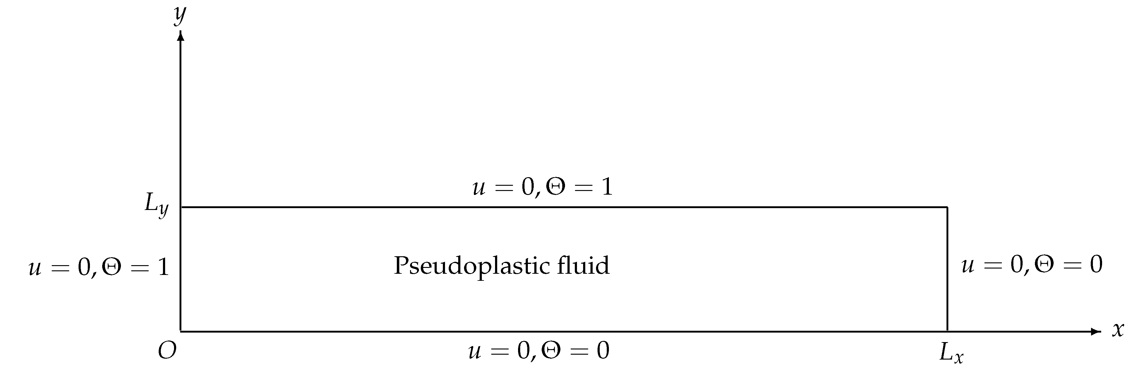
2. Mathematical Modelling

Figure 1 illustrates the schematic diagram of the model problem.

We work in rectangular coordinates, and all quantities are assumed to be dimensionless. In particular, the field variables $x,y,u,\mathsf{\Theta }$ respectively represent the dimensionless horizontal coordinate, vertical coordinate, horizontal velocity component, and temperature. A pseudoplastic (shear-thinning) non-Newtonian fluid is confined to the rectangular domain;

$$\mathsf{\Omega }=\{(x,y):0\le x\le L_x,0\le y\le L_y\},$$

where $L_x$ and $L_y$ are dimensionless lengths with $L_y\ll L_x$. Under these conditions, the transverse velocity component, v, is assumed small compared to u, i.e., $v\ll u$. We consider a situation in which the boundaries $x=0$ and $y=L_y$ are heated, and the remaining boundaries $y=0$ and $x=L_x$ are cooled. Being a non-Newtonian fluid, the assumption of fluid incompressibility is automatically invoked. If this setup can sustain for a relatively long time, then the velocity field $(u,v)$ and the temperature $\mathsf{\Theta }$ would satisfy a coupled set of boundary value problems derived from the mass, momentum, and energy conservation equations of fluid dynamics. Under the current assumptions, the relevant and steady mass, momentum, and energy conservation equations are respectively given by Equations (1)–(3),

$$\begin{array}{cc}\hfill \frac{\partial u}{\partial x}+\frac{\partial v}{\partial y}& =0,\hfill \\ \hfill & \hfill \end{array}$$

(1)

$$\begin{array}{cc}\hfill u\frac{\partial u}{\partial x}+v\frac{\partial u}{\partial y}& =\frac{1}{\mathrm{Re}}\frac{\partial }{\partial y}\left(\eta (\dot{\gamma },\mathsf{\Theta })\frac{\partial u}{\partial y}\right)+\frac{\mathrm{Gr}}{{\mathrm{Re}}^2}\mathsf{\Theta },\hfill \\ \hfill & \hfill \end{array}$$

(2)

$$\begin{array}{cc}\hfill u\frac{\partial \mathsf{\Theta }}{\partial x}+v\frac{\partial \mathsf{\Theta }}{\partial y}& =\frac{1}{\mathrm{Re}\mathrm{Pr}}\left(\frac{{\partial }^2\mathsf{\Theta }}{\partial x^2}+\frac{{\partial }^2\mathsf{\Theta }}{\partial y^2}\right)+\frac{\eta (\dot{\gamma },\mathsf{\Theta })}{\mathrm{Re}\mathrm{Pr}}{\left(\frac{\partial u}{\partial y}\right)}^2,\hfill \end{array}$$

(3)

subject to the boundary conditions,

$$\begin{array}{cc}\hfill & u(0,y)=0,u(L_x,y)=0,u(x,0)=0,u(x,L_y)=0,v(0,y)=0,\hfill \\ \hfill & \hfill \\ \hfill & \mathsf{\Theta }(x,0)=0,\mathsf{\Theta }(x,L_y)=1,\mathsf{\Theta }(0,y)=1,\mathsf{\Theta }(L_x,y)=0.\hfill \end{array}$$

(4)

Here, the dimensionless parameters, $\mathrm{Re},\mathrm{Gr}$, and $\mathrm{Pr}$ are the Reynolds, Grashof, and Prandtl numbers, respectively, with,

$$\begin{array}{c}\hfill \mathrm{Re}=\frac{{\rho }_0{U}_{max}{L}_y}{{\eta }_0},\mathrm{Pr}=\frac{c_p{\eta }_0}{\kappa },\mathrm{Gr}=\frac{{\rho }_0^{2}g{c}_{\beta }{L}_y^3\mathsf{\Delta }\mathsf{\Theta }}{{\eta }_0^2},\end{array}$$

where ${\rho }_0$ is a constant density, $U_{max}$ is a characteristic maximum velocity, ${\eta }_0$ is a constant viscosity, $c_p$ is the specific heat capacity at constant pressure, $\kappa$ is the thermal conductivity of the fluid, g is the gravitational acceleration, $c_{\beta }$ is the coefficient of thermal expansion, and $\mathsf{\Delta }\mathsf{\Theta }$ is the temperature difference between the hottest and coldest walls, see for example [21].

Given that the transverse velocity, v, may be obtained by integrating the first order Equation (1), we only impose the no-slip boundary condition at the left vertical wall. Also $\eta$ represents the fluid viscosity which, for the non-Newtonian fluids under consideration, depends on the temperature ($\mathsf{\Theta }$) and shear-rates ($\dot{\gamma }$), where, under the current assumptions,

$$\dot{\gamma }\approx \left|\frac{\partial u}{\partial y}\right|.$$

The non-Newtonian viscosity, $\eta$, will be modelled via an appropriate constitutive equation that captures both the shear-thinning properties of the pseudoplastic fluid as well as the temperature dependence. The shear-rate dependence of the viscosity is herein described by a Cross model [29], and the temperature dependence follows a Nahme-type law,

$$\eta (\dot{\gamma },\mathsf{\Theta })=\left(\frac{1}{1+\beta {\dot{\gamma }}^n}\right)e^{-\alpha \mathsf{\Theta }},$$

(5)

where $\alpha ,\beta$, and n are material parameters. As demonstrated in [29,30], the values of n are limited to the range of the values $0\le n<1$. Shear-thinning (pseudoplastic) behaviour is ensured for the values $0<n<1$ with strongly shear-thinning behaviour obtaining as $n\to 1$. Taking $n=0$ and/or $\beta =0$ leads to Newtonian viscosity. The viscosity of all fluids is expected to decrease with increasing temperature, hence $\alpha \ge 0$. The value $\alpha =0$ is synonymous with assumptions of isothermal (temperature-independent) viscosity.

3. Numerical Solution

The nonlinear and coupled boundary value problem (BVP) given by Equations (1)–(4) is not amenable to analytic solution techniques. Direct numerical treatment of the equations as given is also very challenging. We deploy an innovative, robust, and efficient numerical approach that recasts the boundary value problem as a time-dependent initial-boundary value problem (IBVP). We then extract the steady solutions of the IBVP. Indeed, the steady-state solutions of the IBVP are the same as the solutions of the original BVP. The main advantage here is that the IBVP solutions are obtained efficiently, accurately, and with relative ease. In this work, we employ numerical solutions based on the Finite Difference Methods (FDM). Similar time-dependent numerical solutions for non-isothermal non-Newtonian (viscoelastic) fluid flow have been recently developed via Finite Volume Methods, see for example [24,25].

Equations (1)–(3) are, therefore, recast as the equivalent time-dependent IBVP,

$$\begin{array}{cc}\hfill \frac{\partial u}{\partial x}+\frac{\partial v}{\partial y}& =0,\hfill \\ \hfill & \hfill \end{array}$$

(6)

$$\begin{array}{cc}\hfill \frac{\partial u}{\partial t}+u\frac{\partial u}{\partial x}+v\frac{\partial u}{\partial y}& =\frac{1}{\mathrm{Re}}\frac{\partial }{\partial y}\left(\eta (\dot{\gamma },\mathsf{\Theta })\frac{\partial u}{\partial y}\right)+\frac{\mathrm{Gr}}{{\mathrm{Re}}^2}\mathsf{\Theta },\hfill \\ \hfill & \hfill \end{array}$$

(7)

$$\begin{array}{cc}\hfill \frac{\partial \mathsf{\Theta }}{\partial t}+u\frac{\partial \mathsf{\Theta }}{\partial x}+v\frac{\partial \mathsf{\Theta }}{\partial y}& =\frac{1}{\mathrm{Re}\mathrm{Pr}}\left(\frac{{\partial }^2\mathsf{\Theta }}{\partial x^2}+\frac{{\partial }^2\mathsf{\Theta }}{\partial y^2}\right)+\frac{\eta (\dot{\gamma },\mathsf{\Theta })}{\mathrm{Re}\mathrm{Pr}}{\left(\frac{\partial u}{\partial y}\right)}^2.\hfill \end{array}$$

(8)

In addition to the boundary conditions in Equation (4), the IBVP as represented by Equations (6)–(8) would need to be supplemented by appropriate initial conditions. We employ zero initial conditions,

$$u(t,x,y)=0,v(t,x,y)=0,\mathsf{\Theta }(t,x,y)=0,\mathrm{for}t=0\mathrm{and}\forall (x,y)\in \mathsf{\Omega }\setminus \delta \mathsf{\Omega },$$

(9)

where,

$$\delta \mathsf{\Omega }=\{x=0\}\cup \{x=L_x\}\cup \{y=0\}\cup \{y=L_y\},$$

is the boundary to the domain $\mathsf{\Omega }$. The boundary conditions are also recast to include the time as,

$$\begin{array}{cc}\hfill & u(t,0,y)=0,u(t,L_x,y)=0,u(t,x,0)=0,u(t,x,L_y)=0,v(t,0,y)=0,\hfill \\ \hfill & \hfill \\ \hfill & \mathsf{\Theta }(t,x,0)=0,\mathsf{\Theta }(t,x,L_y)=1,\mathsf{\Theta }(t,0,y)=1,\mathsf{\Theta }(t,L_x,y)=0,\mathrm{for}t\ge 0\mathrm{and}(x,y)\in \delta \mathsf{\Omega }.\hfill \end{array}$$

(10)

Numerical Algorithm

To solve Equations (6)–(8) subject to the boundary conditions given in Equation (10) and the initial conditions given in Equation (9), we employ finite difference numerical techniques. In particular, the computational algorithms are based on the semi-implicit finite difference methods. Details of our numerical algorithms are illustrated, say, in [21,22]. Taking N as the current time level, $N+1$ as the subsequent time level, and $N+\xi$ with $0\le \xi \le 1$ as an intermediate time level, the semi-implicit scheme for the u-velocity component reads,

$$\begin{array}{cc}\hfill \frac{u^{(N+1)}-u^{\left(N\right)}}{\mathsf{\Delta }t}+{\left[u\frac{\partial u}{\partial x}+v\frac{\partial u}{\partial y}\right]}^{\left(N\right)}& =\frac{1}{\mathrm{Re}}{\left[\eta (\dot{\gamma },\mathsf{\Theta })\right]}^{\left(N\right)}{\left[\frac{{\partial }^{2}u}{\partial y^2}\right]}^{(N+\xi )}\hfill \\ \hfill & \\ \hfill & +\frac{1}{\mathrm{Re}}{\left[\frac{\partial }{\partial y}\eta (\dot{\gamma },\mathsf{\Theta })\frac{\partial u}{\partial y}\right]}^{\left(N\right)}+\frac{\mathrm{Gr}}{{\mathrm{Re}}^2}{\mathsf{\Theta }}^{\left(N\right)}.\hfill \end{array}$$

(11)

The equation for $u^{(N+1)}$ then becomes:

$$-r_1{u}_{i,j-1}^{(N+1)}+(1+2r_1)u_{i,j}^{(N+1)}-r_1{u}_{i,j+1}^{(N+1)}=\mathrm{explicit}\mathrm{terms},$$

(12)

where

$$r_1=\frac{\xi }{\mathrm{Re}}{\left[\eta (\dot{\gamma },\mathsf{\Theta })\right]}_{i,j}^{\left(N\right)}\frac{\mathsf{\Delta }t}{\mathsf{\Delta }{y}^2}.$$

The solution procedure for $u^{(N+1)}$ reduces to efficient linear algebraic processes of inversion of nonsingular, diagonally dominant, and tri-diagonal matrices. The semi-implicit scheme for the temperature equation is similarly approached; unmixed second partial derivatives of the temperature are treated implicitly,

$$\begin{array}{cc}\hfill \frac{{\mathsf{\Theta }}^{(N+1)}-{\mathsf{\Theta }}^{\left(N\right)}}{\mathsf{\Delta }t}+{\left[u\frac{\partial \mathsf{\Theta }}{\partial x}+v\frac{\partial \mathsf{\Theta }}{\partial y}\right]}^{\left(N\right)}& =\frac{1}{\mathrm{Re}\mathrm{Pr}}{\left[\frac{{\partial }^2\mathsf{\Theta }}{\partial x^2}+\frac{{\partial }^2\mathsf{\Theta }}{\partial y^2}\right]}^{(N+\xi )}\hfill \\ \hfill & \hfill \\ \hfill & +\frac{1}{\mathrm{Re}\mathrm{Pr}}{\left[\eta (\dot{\gamma },\mathsf{\Theta }){\left(\frac{\partial u}{\partial y}\right)}^2\right]}^{\left(N\right)}.\hfill \end{array}$$

(13)

The algorithm (13) allows for the decoupling of variables, which represents a significant advantage over a fully implicit scheme. The implicit terms are,

$$1-\frac{1}{\mathrm{Re}\mathrm{Pr}}\xi \mathsf{\Delta }t\left(\frac{{\partial }^2}{\partial x^2}+\frac{{\partial }^2}{\partial y^2}\right){\mathsf{\Theta }}^{(N+1)}.$$

The operator on ${\mathsf{\Theta }}^{(N+1)}$ factorizes with an associated error term of order,

$$\mathrm{factorization}\mathrm{error}=O\left({\left(\frac{\xi \mathsf{\Delta }t}{\mathrm{Re}\mathrm{Pr}}\right)}^2\right).$$

(14)

Small $\mathsf{\Delta }t$ and relatively large $\mathrm{Re}\mathrm{Pr}$ lead to very small factorization errors. The semi-implicit algorithm for the temperature equation, therefore, reduces to,

$$\left(1-\frac{1}{\mathrm{Re}\mathrm{Pr}}\xi \mathsf{\Delta }t\frac{{\partial }^2}{\partial x^2}\right)\left(1-\frac{1}{\mathrm{Re}\mathrm{Pr}}\xi \mathsf{\Delta }t\frac{{\partial }^2}{\partial y^2}\right){\mathsf{\Theta }}^{(N+1)}=\mathrm{explicit}\mathrm{terms}.$$

(15)

The solution procedure again reduces to the efficient linear algebraic processes of inversion of nonsingular, diagonally dominant, and tri-diagonal matrices.

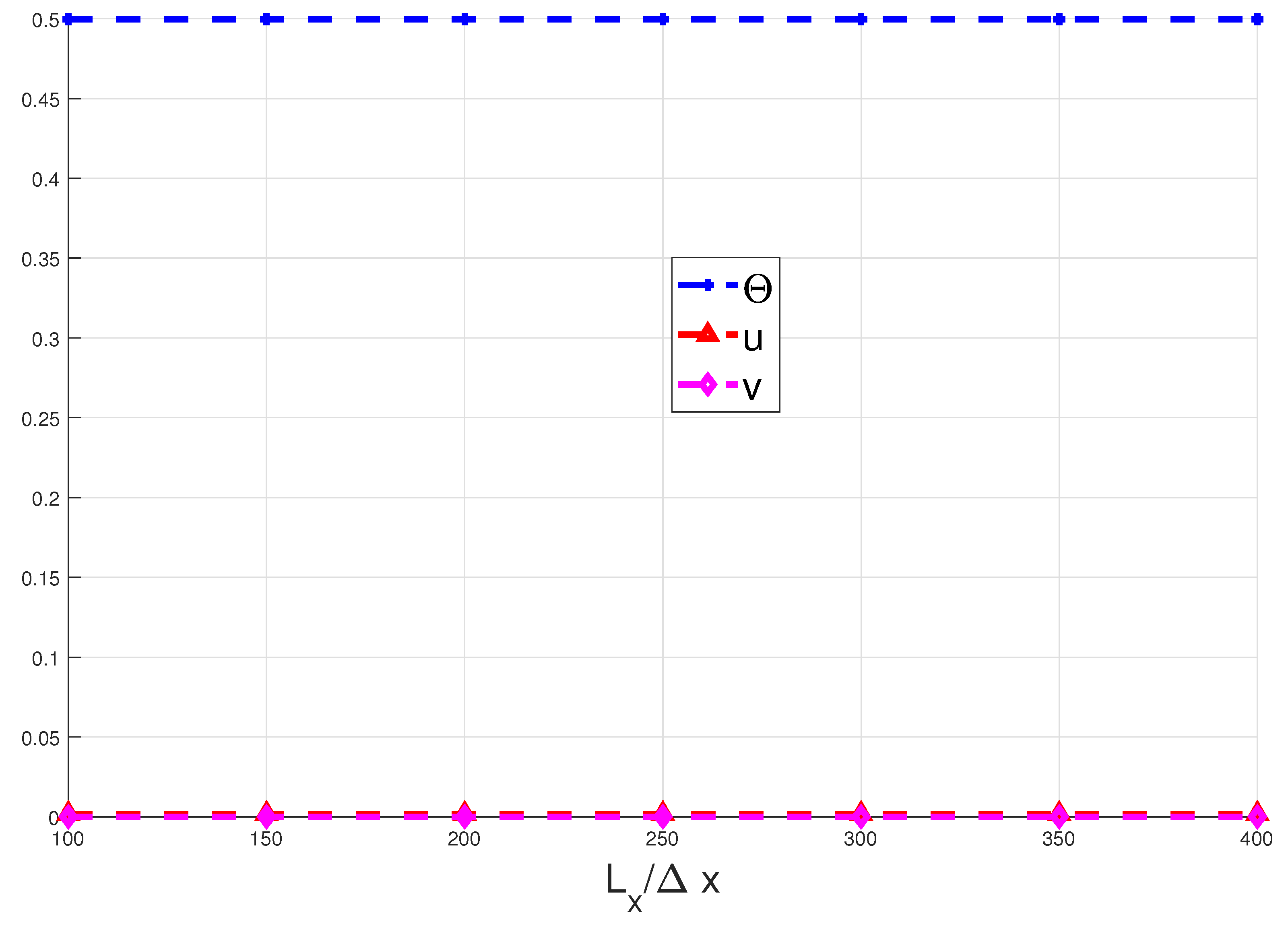
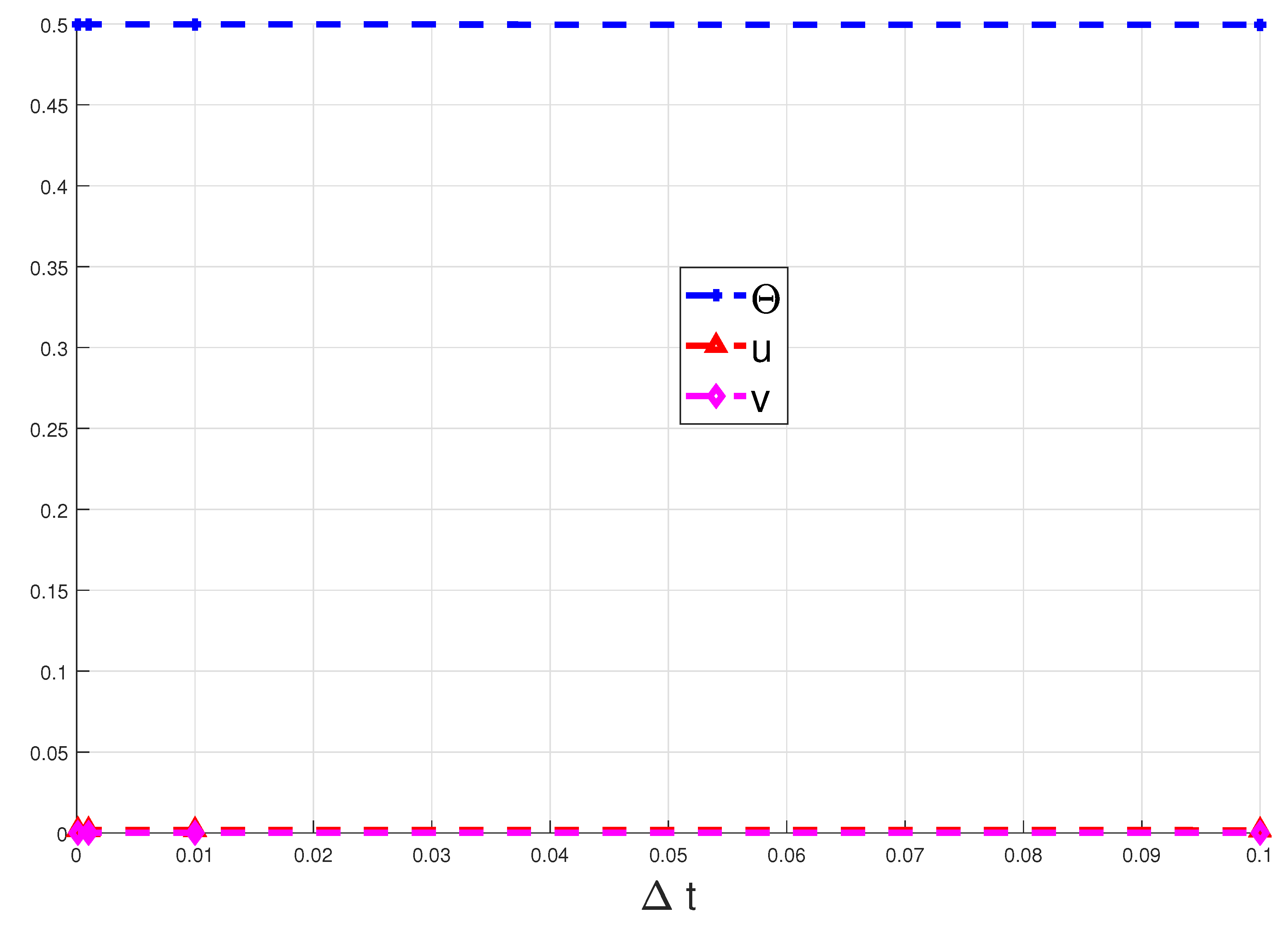
4. Numerical Stability

Before we proceed to the computational results obtained from our numerical algorithms, it is fundamentally important to demonstrate the numerical stability of the underlying algorithms. Specifically, we need to demonstrate that the computational results are independent of both mesh size and time-step size. Figure 2 and Figure 3, respectively, illustrate that our numerical algorithms are indeed independent of mesh size and time-step size.

The results of Figure 2 and Figure 3 indeed illustrate, as expected, that our numerical algorithms are independent of mesh size and time-step size. The mesh sizes used in Figure 2 range from $101\times 101$ to $401\times 401$ grid points. These grid points respectively correspond to $100\times 100$ to $400\times 400$ computational cells. The time-step sizes employed in Figure 3 range from $0.0001$ to $0.1$.

The values for temperature and velocity plotted in Figure 2 and Figure 3 correspond to the values at the midpoint of the computational domain at time $t=5$, i.e.,

$$\mathsf{\Theta }(x,y,t)=\mathsf{\Theta }\left(\frac{L_x}{2},\frac{L_y}{2},5\right),u(x,y,t)=u\left(\frac{L_x}{2},\frac{L_y}{2},5\right),v(x,y,t)=v\left(\frac{L_x}{2},\frac{L_y}{2},5\right).$$

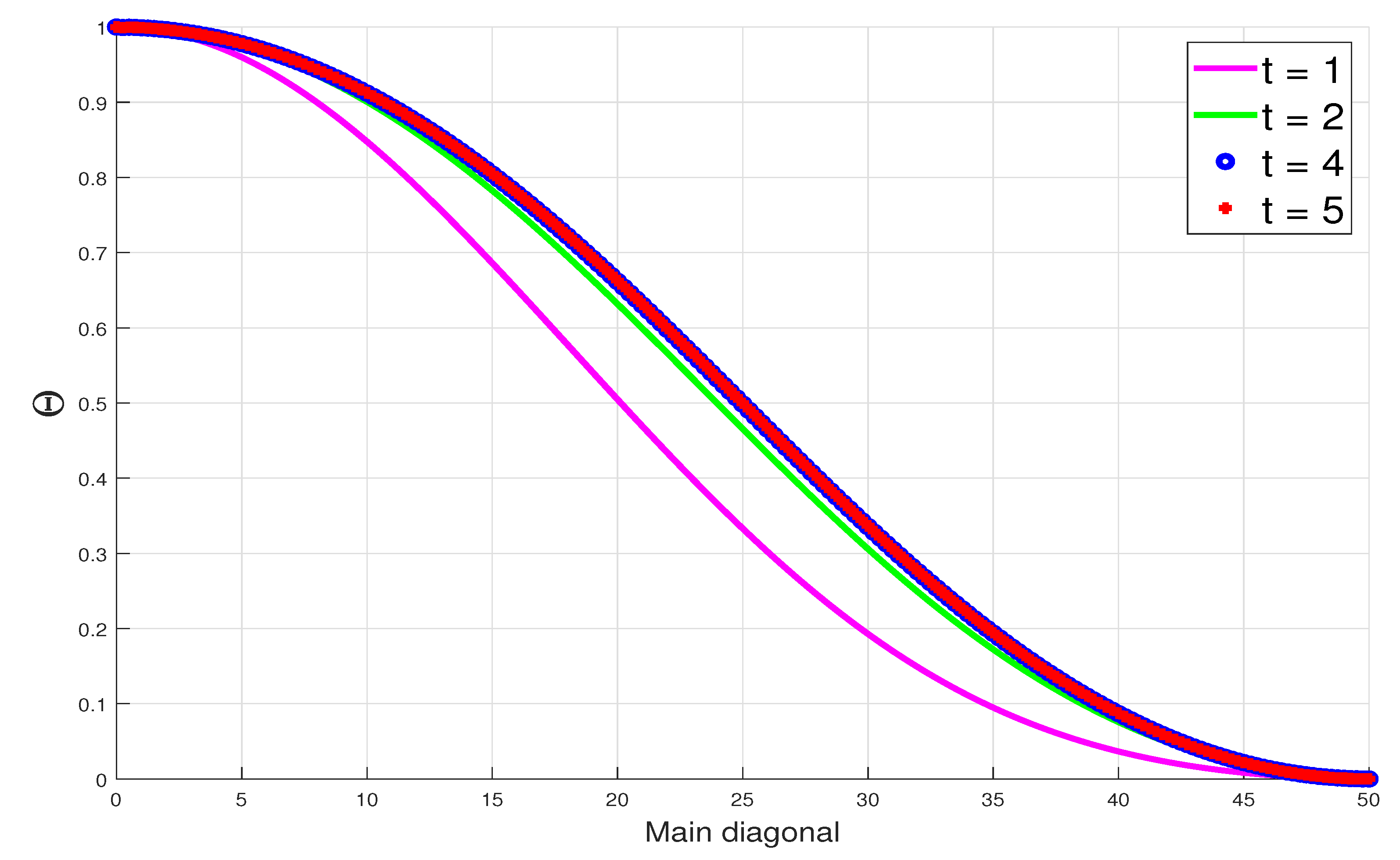
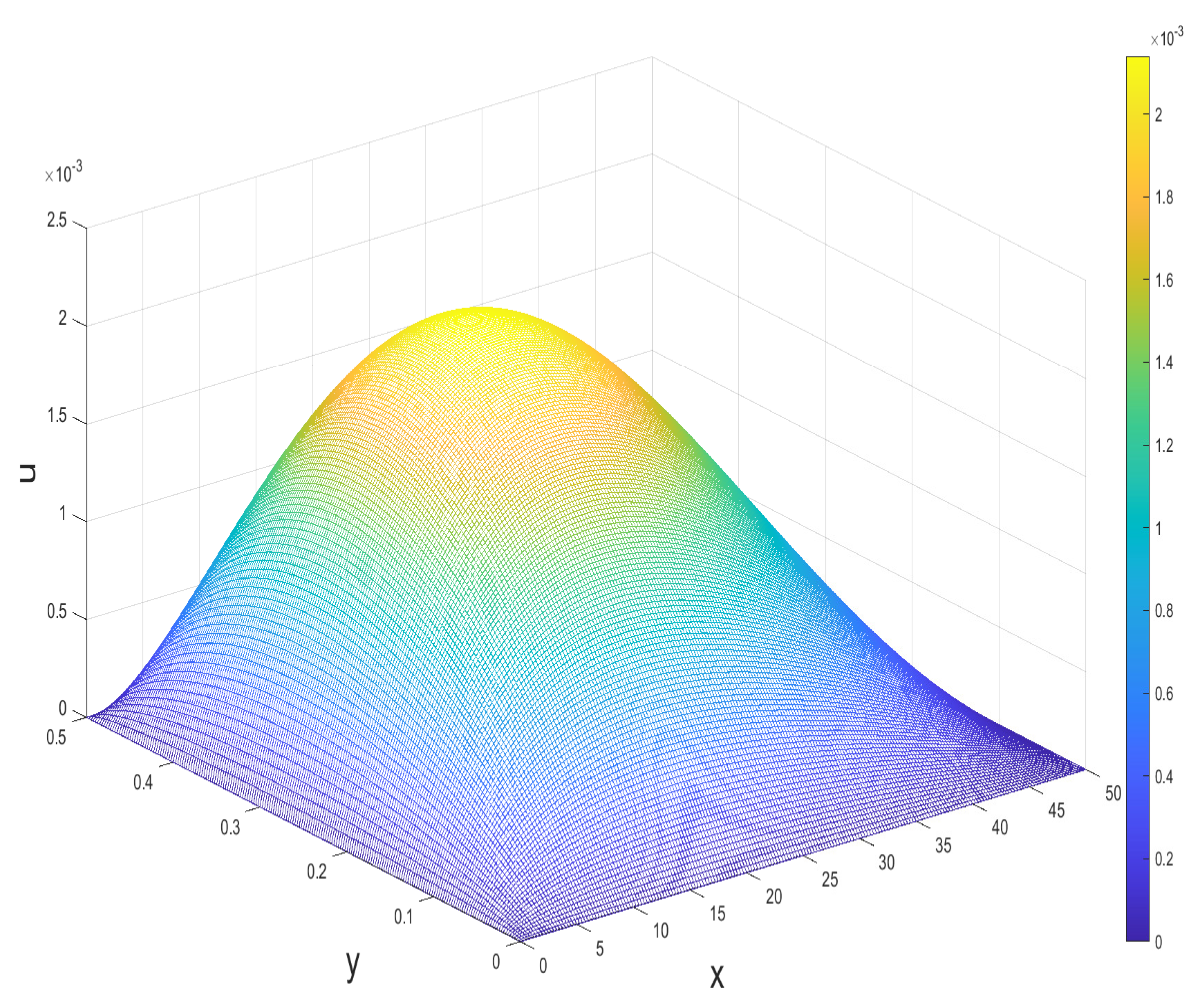
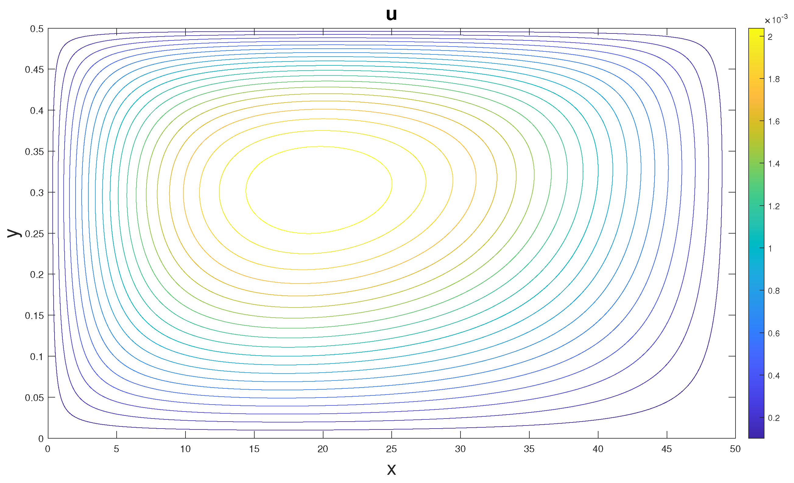
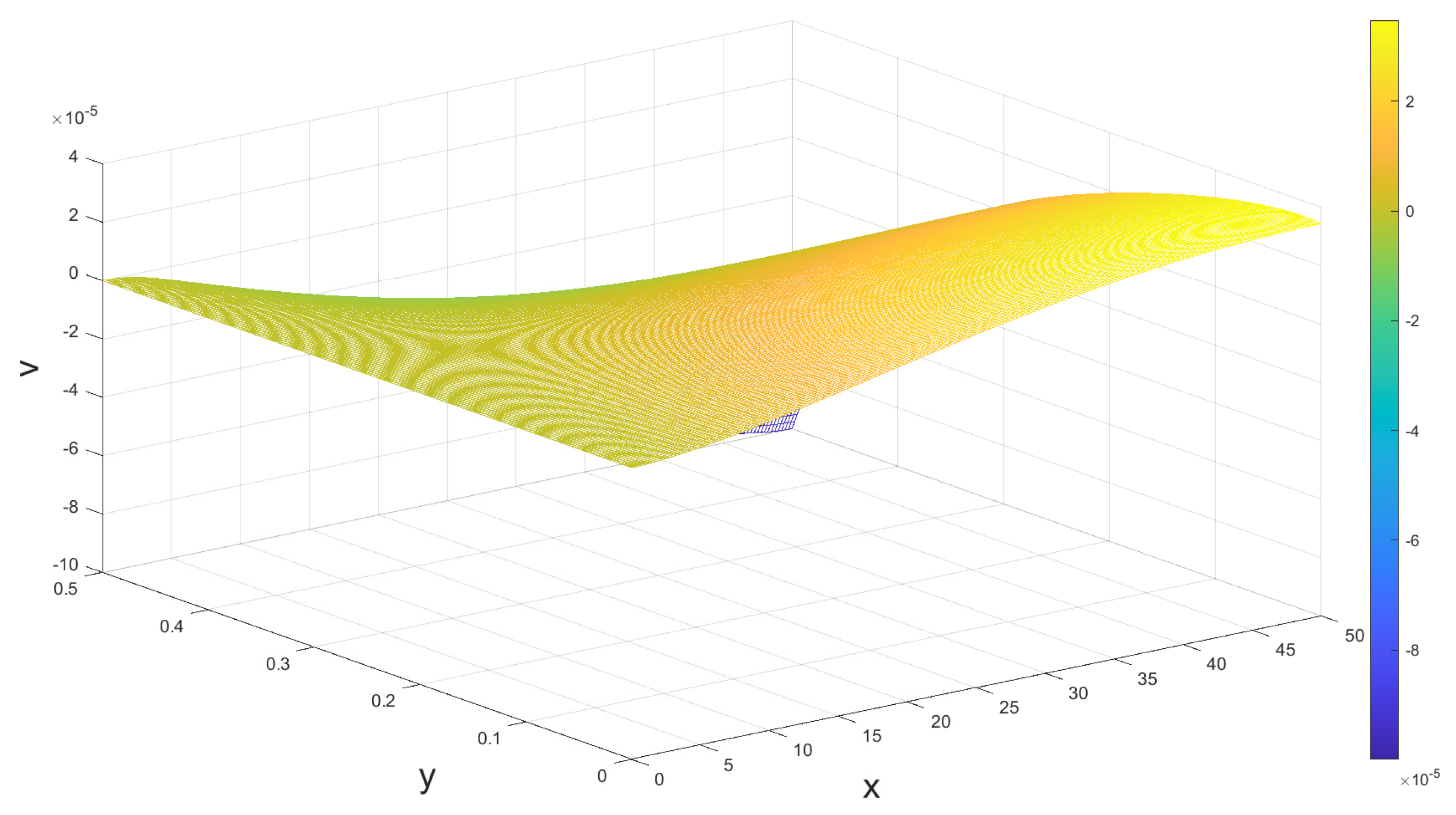
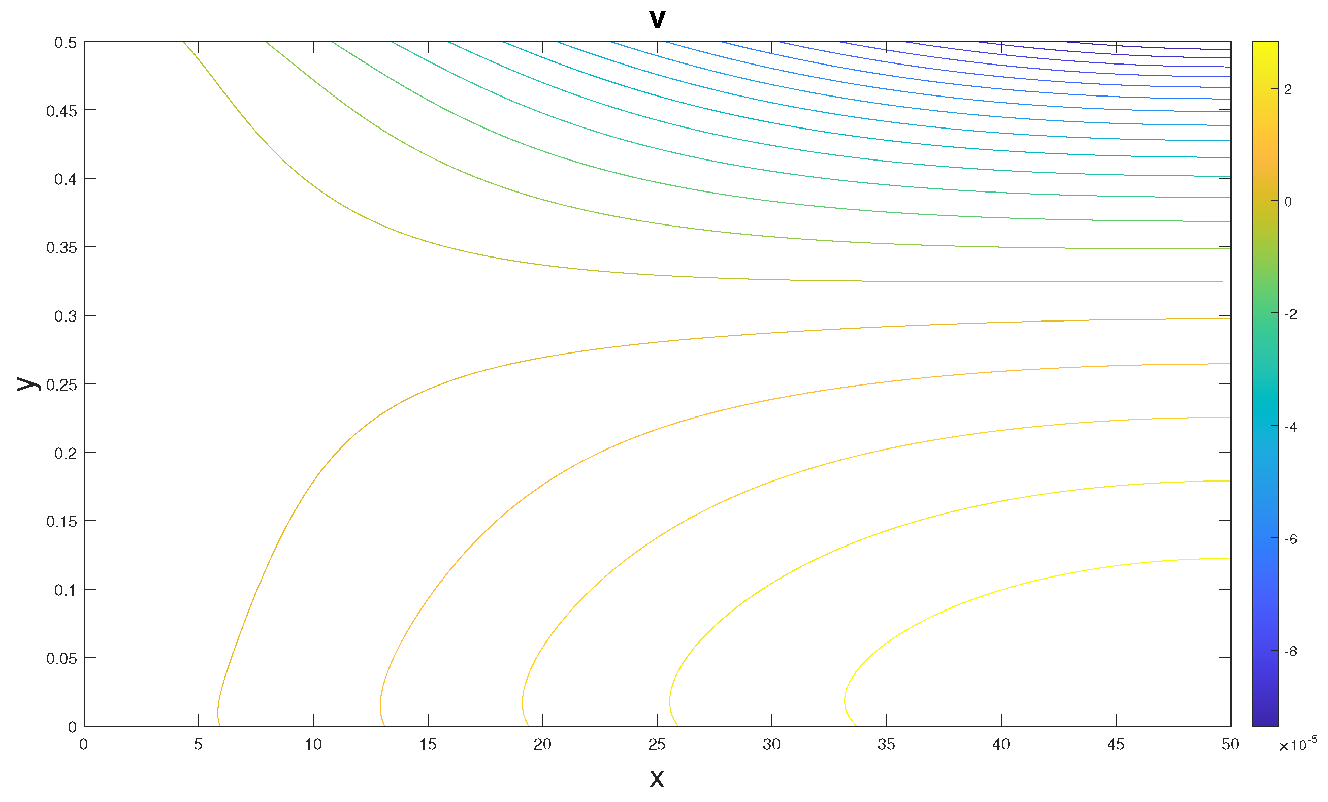
5. Computational Results

To improve computational costs, we need to avoid using very small time-step ($\mathsf{\Delta }t$) values. The versatility of our semi-implicit finite difference algorithm means that we can take $\xi =1$, which in turn would allow us to use large time-steps. As a comparison, an explicit finite difference method (with $\xi =0$) would require extremely small time-step sizes.

Even though our choice of $\xi =1$ allows for larger time-step sizes and hence low computational costs, we need to balance this with the requirements of minimizing the numerical factorization errors as given by the conditions of Equation (14). We will, therefore, employ reasonably low time-step sizes that will still keep the computational costs manageably low while also ensuring that the numerical factorization errors remain negligibly small.

Unless otherwise stated, we will discretize the domain $\mathsf{\Omega }$ into a $201\times 201$ mesh grid and employ the parameter values,

$$L_y=0.5,L_x=50,\alpha =0.1,\beta =10,\mathrm{Gr}=0.1,{\mathrm{Pr}}_0=25,\mathrm{Re}=1,n=0.5,\mathsf{\Delta }t={10}^{-4}.$$

(16)

Figure 4, Figure 5 and Figure 6 show the time development of solutions until steady states are reached. The figures are plotted along the main diagonal, which connects the hottest and coldest corners, i.e., the $(x,y)$ points $(0,L_y)$ and $(L_x,0)$.

Figure 7, Figure 8, Figure 9, Figure 10, Figure 11 and Figure 12 give the steady-state surface plots and respective contour plots of the temperature and velocity components at time $t=10$. The results confirm the prediction, as summarized in the introduction, that the velocities associated with natural convection flow are relatively low.

6. Parameter Dependence of Solutions

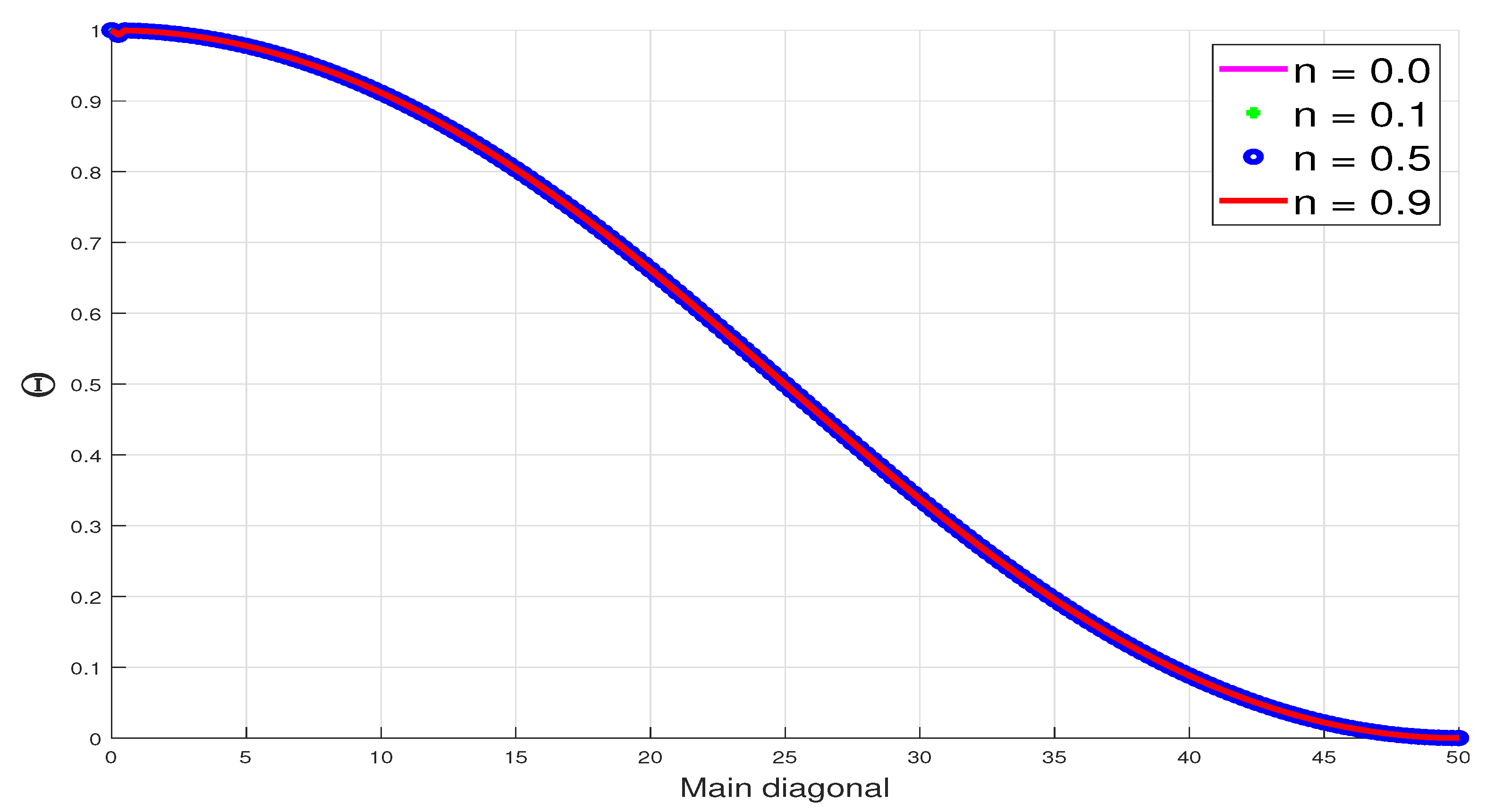
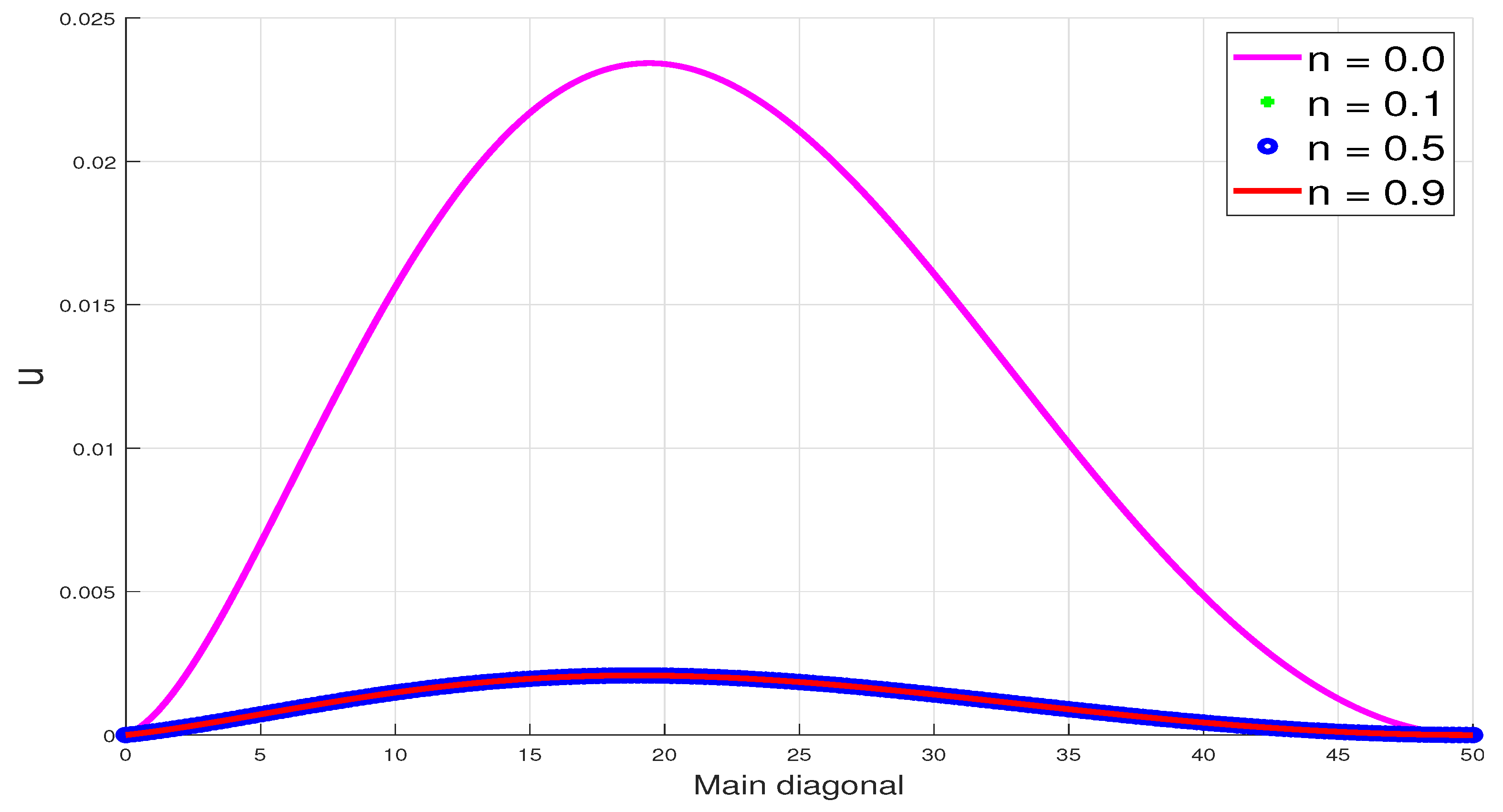
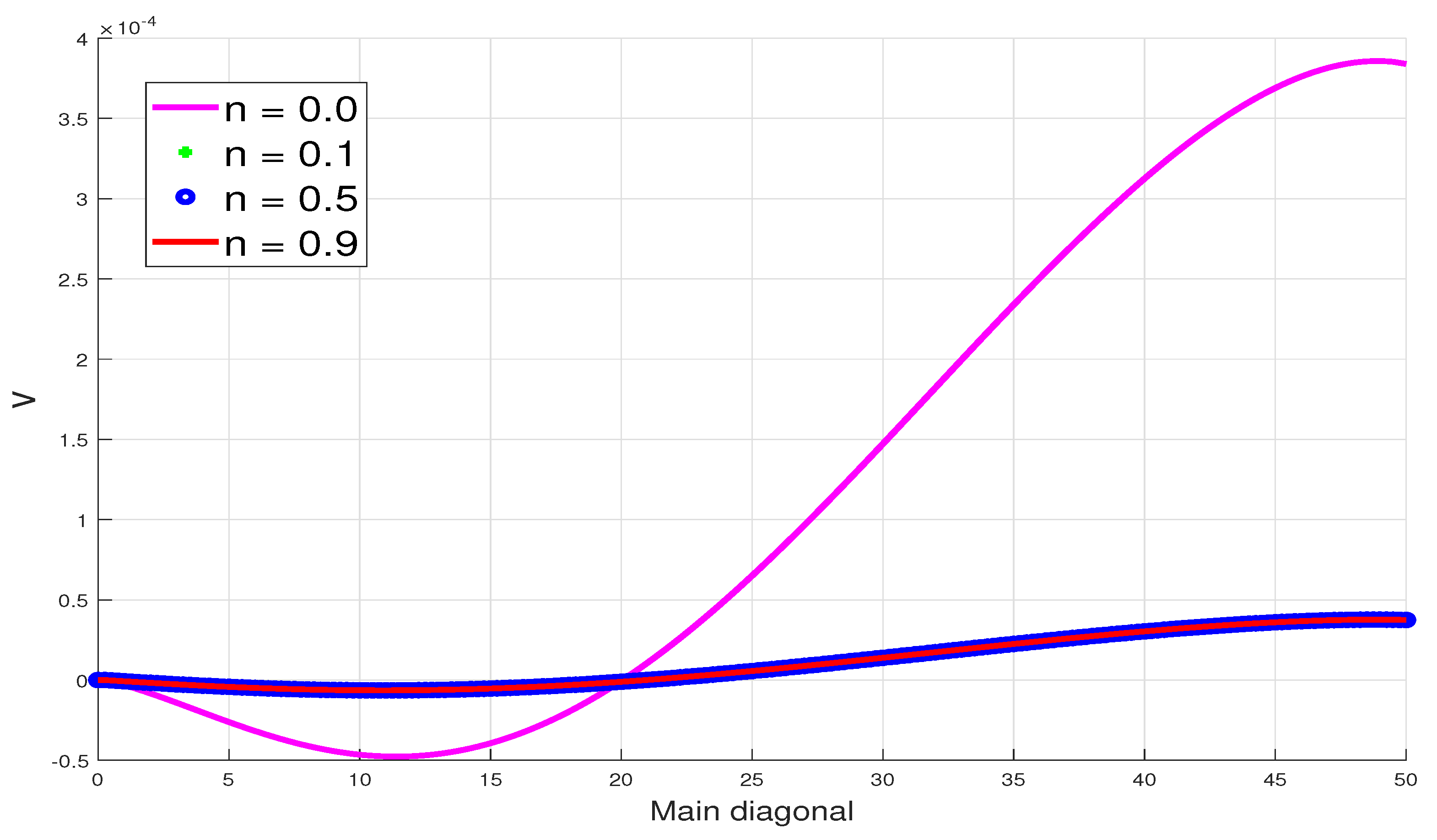
6.1. Dependence on Shear-Thinning Parameter, n

The dependence of solutions on the shear-thinning parameter n is illustrated in Figure 13, Figure 14 and Figure 15. As already predicted and indeed demonstrated in the previous subsection, the velocities associated with natural convection flow are relatively low. This, in turn, implies very low shear rates within the channel flow. This means that the pseudoplastic viscosities would be much larger than the corresponding Newtonian viscosity since,

$$(1+\beta {\dot{\gamma }}^n)\ll (1+\beta )\Rightarrow \frac{1}{1+\beta }\ll \frac{1}{1+\beta {\dot{\gamma }}^n}.$$

The lower viscosity Newtonian fluid, therefore, leads to much larger velocities than the corresponding pseudoplastic fluids as illustrated in Figure 14 and Figure 15. The fluid temperature is largely influenced by the boundary conditions of the heated and cooled walls and hence is not significantly affected by the changes to the fluid viscidity, see Figure 13.

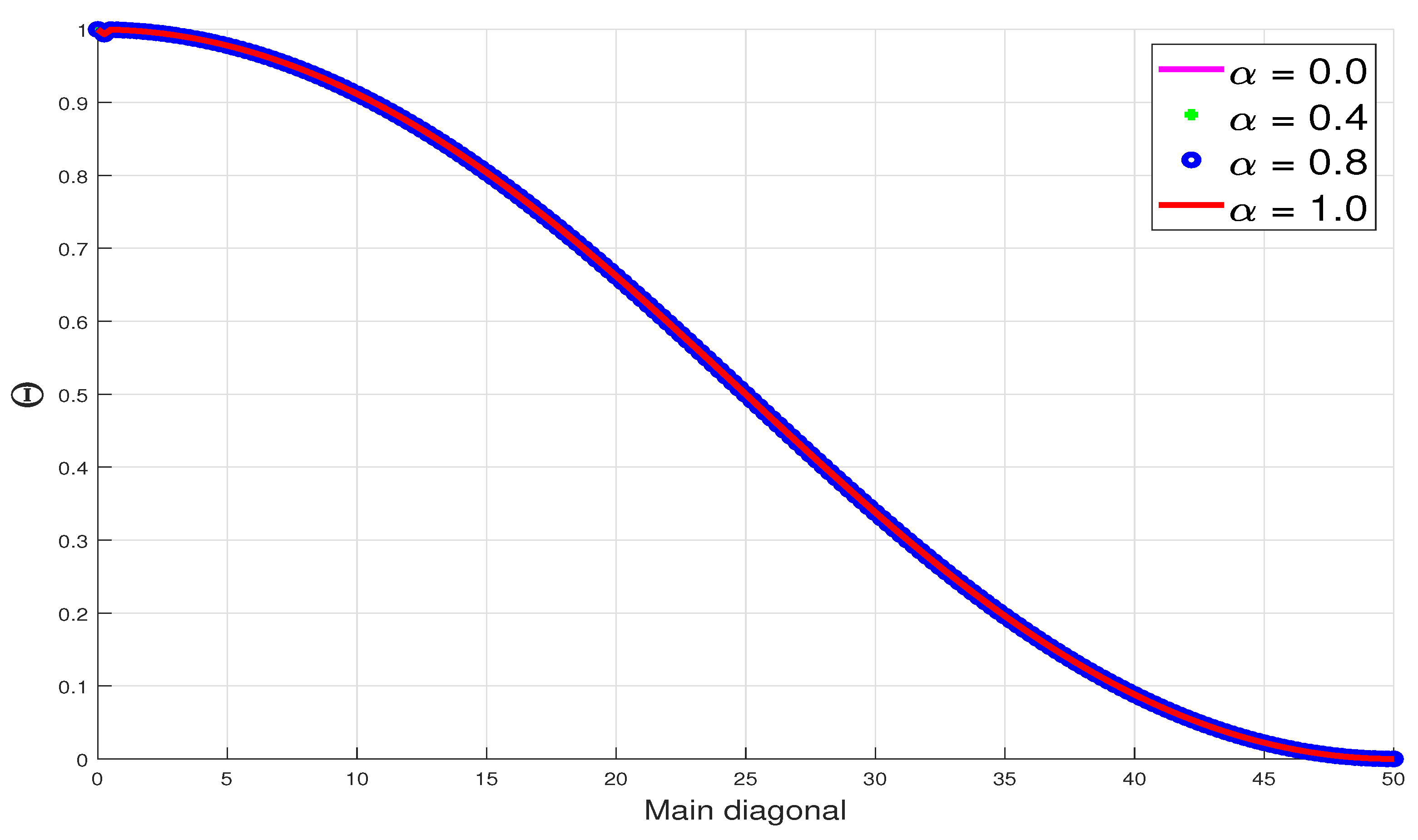
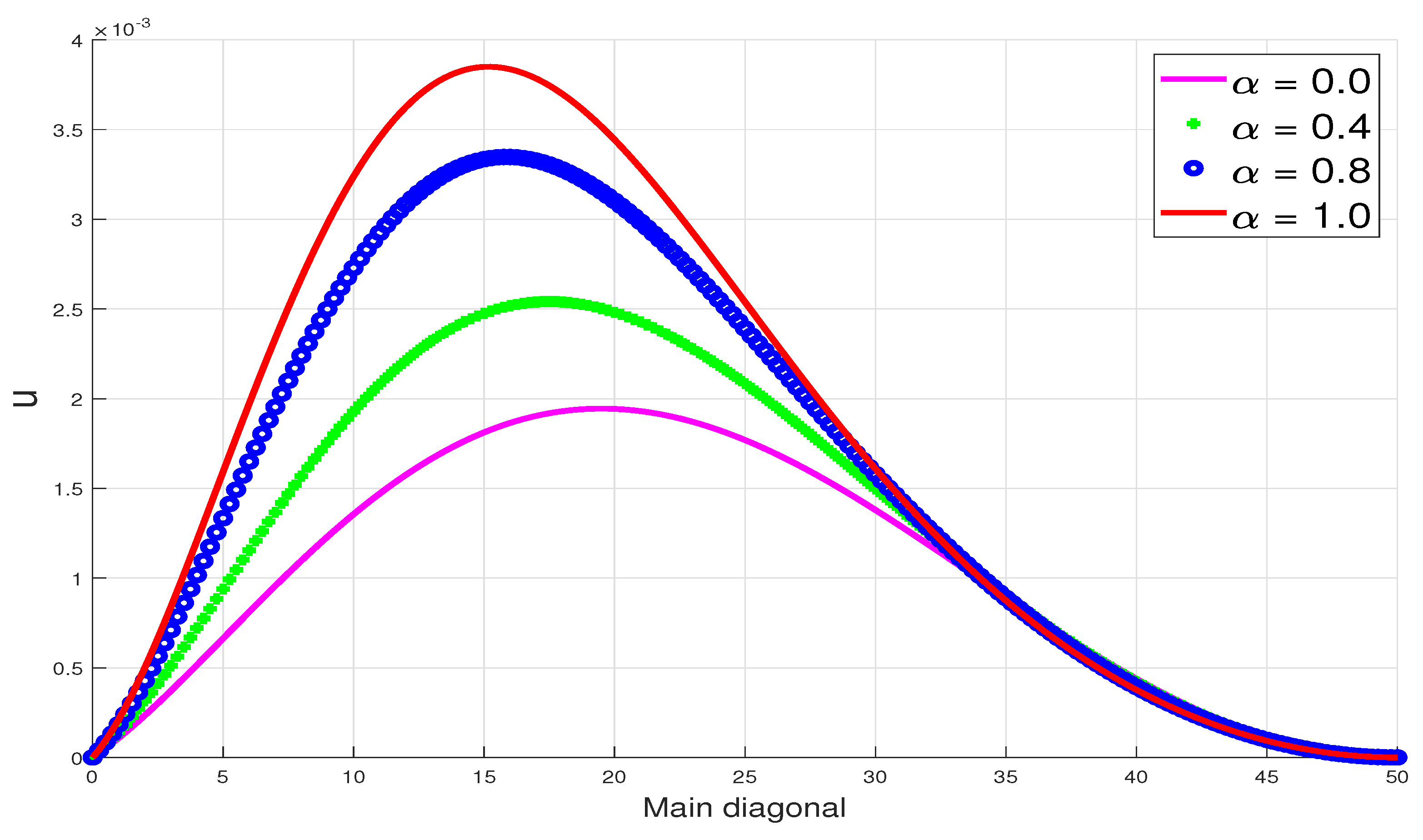
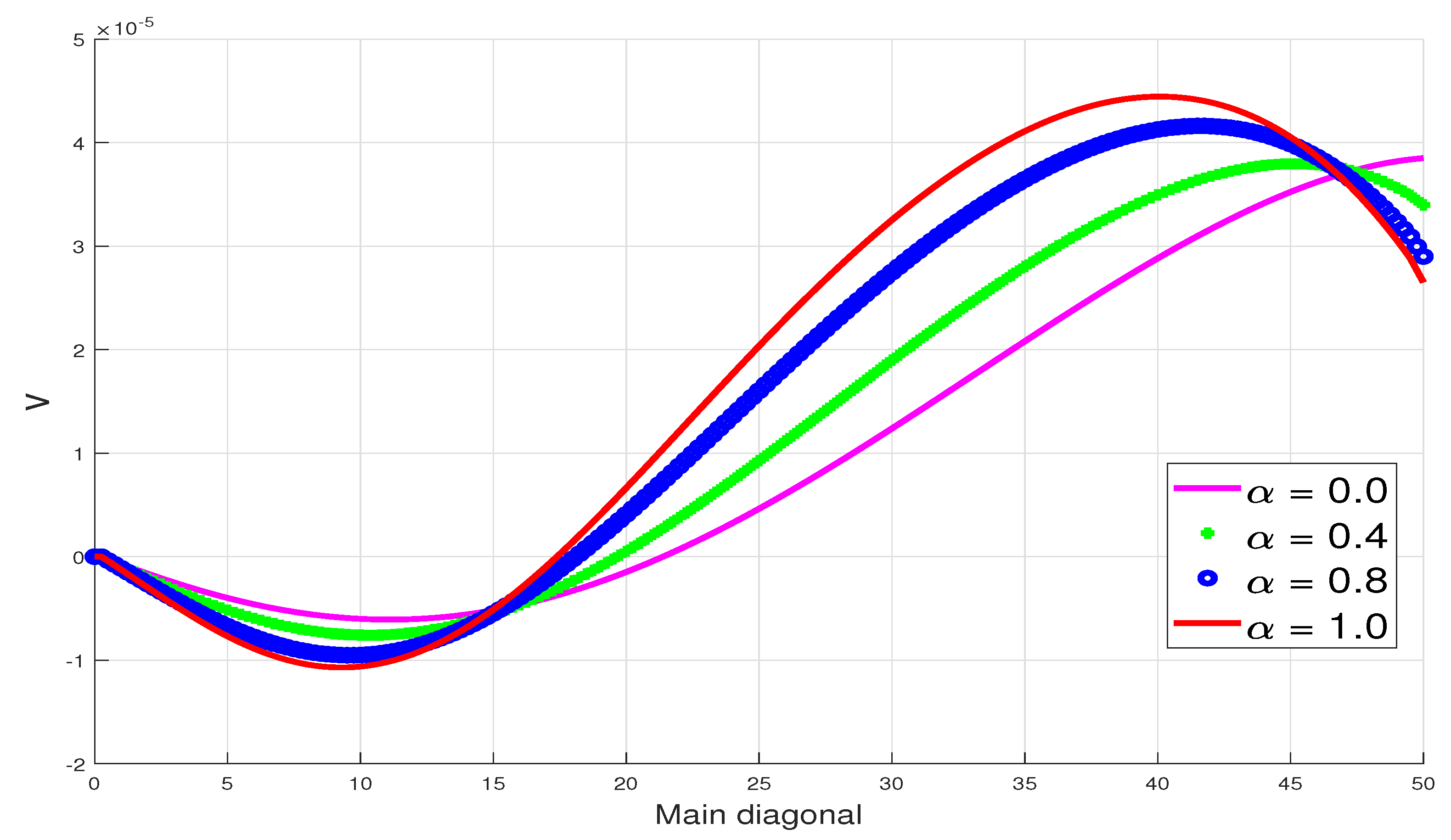
6.2. Dependence on Non-Isothermal Viscosity Parameter, $\alpha$

The dependence of solutions on the non-isothermal viscosity parameter $\alpha$ is illustrated in Figure 16, Figure 17 and Figure 18. The behaviour of solutions is similar to that with respect to the shear-thinning parameter n and hence is similarly explained. In particular, higher values of $\alpha$ result in lower fluid viscosity and vice versa.

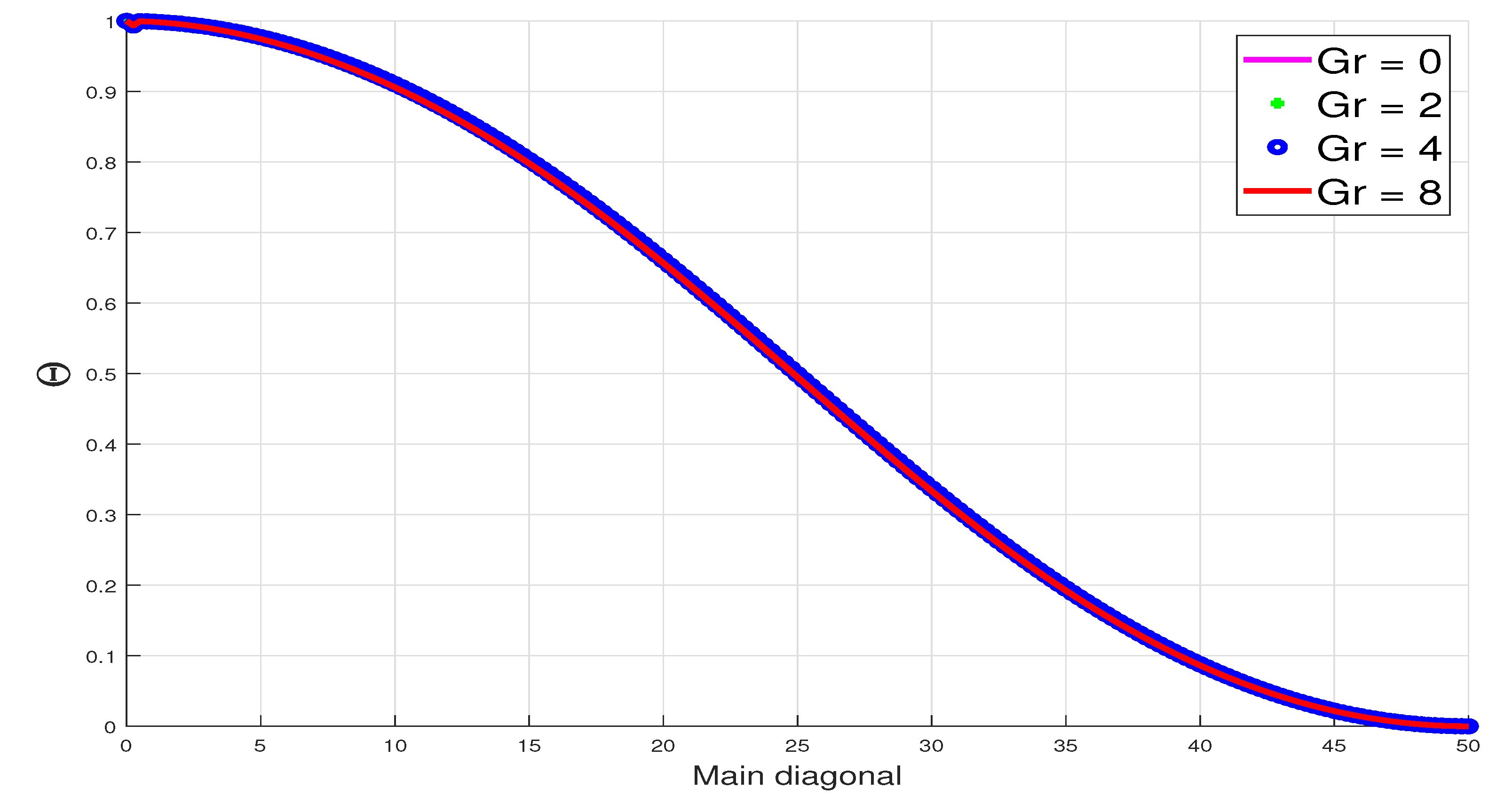
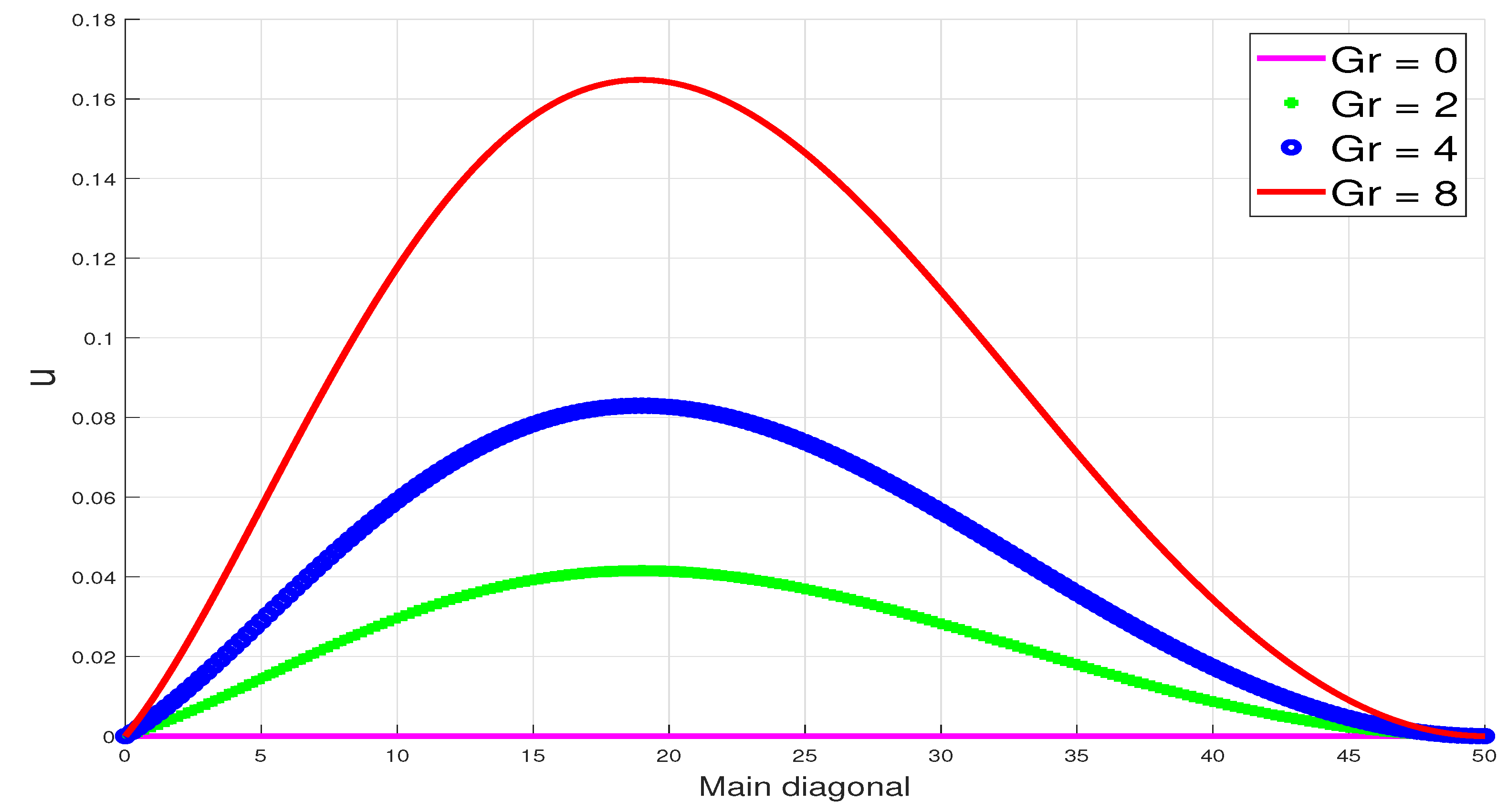
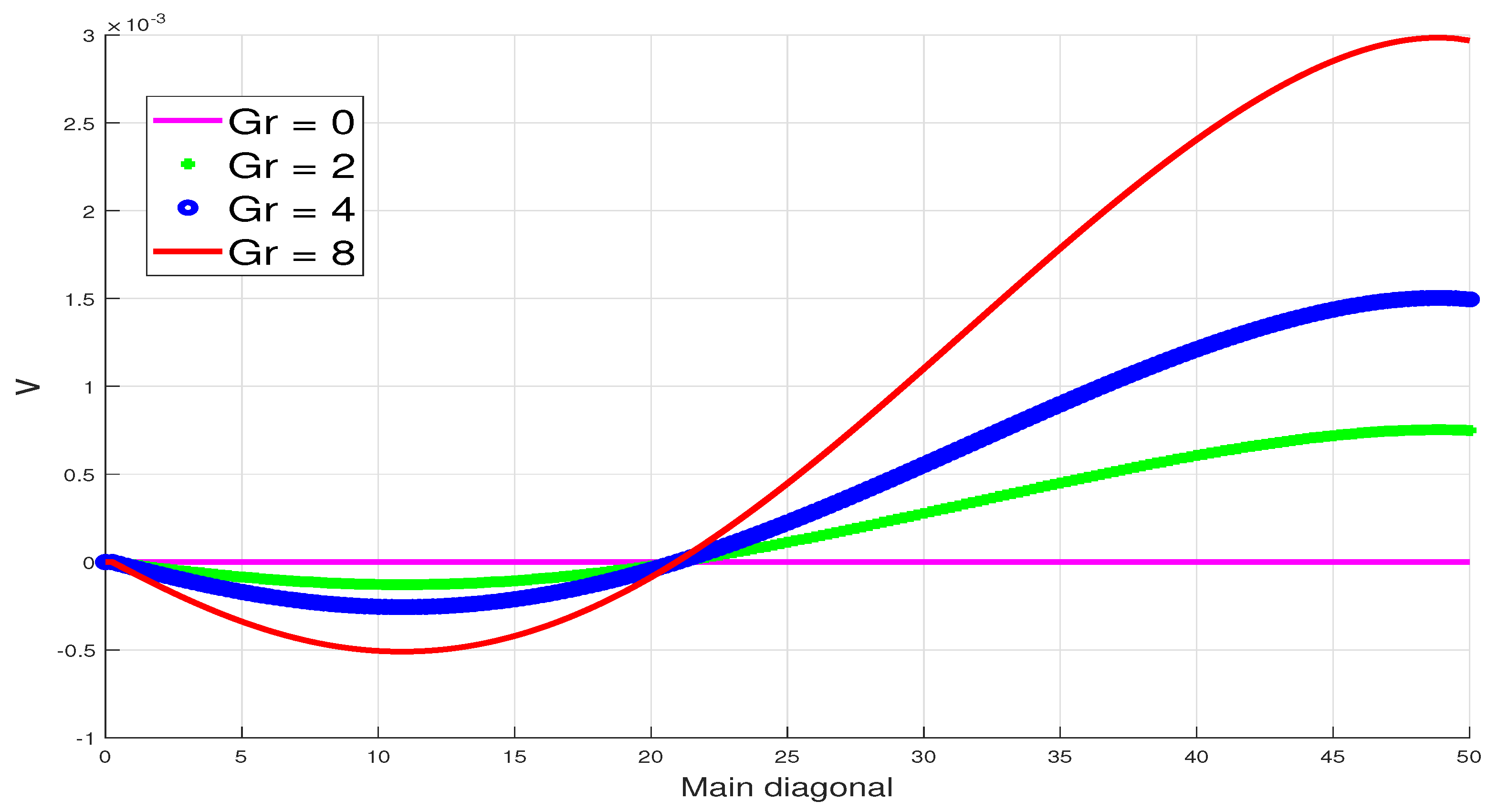
6.3. Dependence on Grashof number, $G$

The dependence of solutions on the buoyancy parameter, i.e., the Grashof number, $\mathrm{Gr}$, is illustrated in Figure 19, Figure 20 and Figure 21. The Grashof number represents the driving force for the fluid velocity. In particular, the fluid velocity is driven purely by natural convection effects and hence should remain zero when there is no convection (Gr=0) and otherwise increase with increasing Gr. These observations are illustrated in Figure 20 and Figure 21. As already observed, the fluid temperature is driven largely by the boundary conditions, and hence the parameter $\mathrm{Gr}$, being connected to the fluid velocity, has limited influence on fluid temperature as shown in Figure 19.

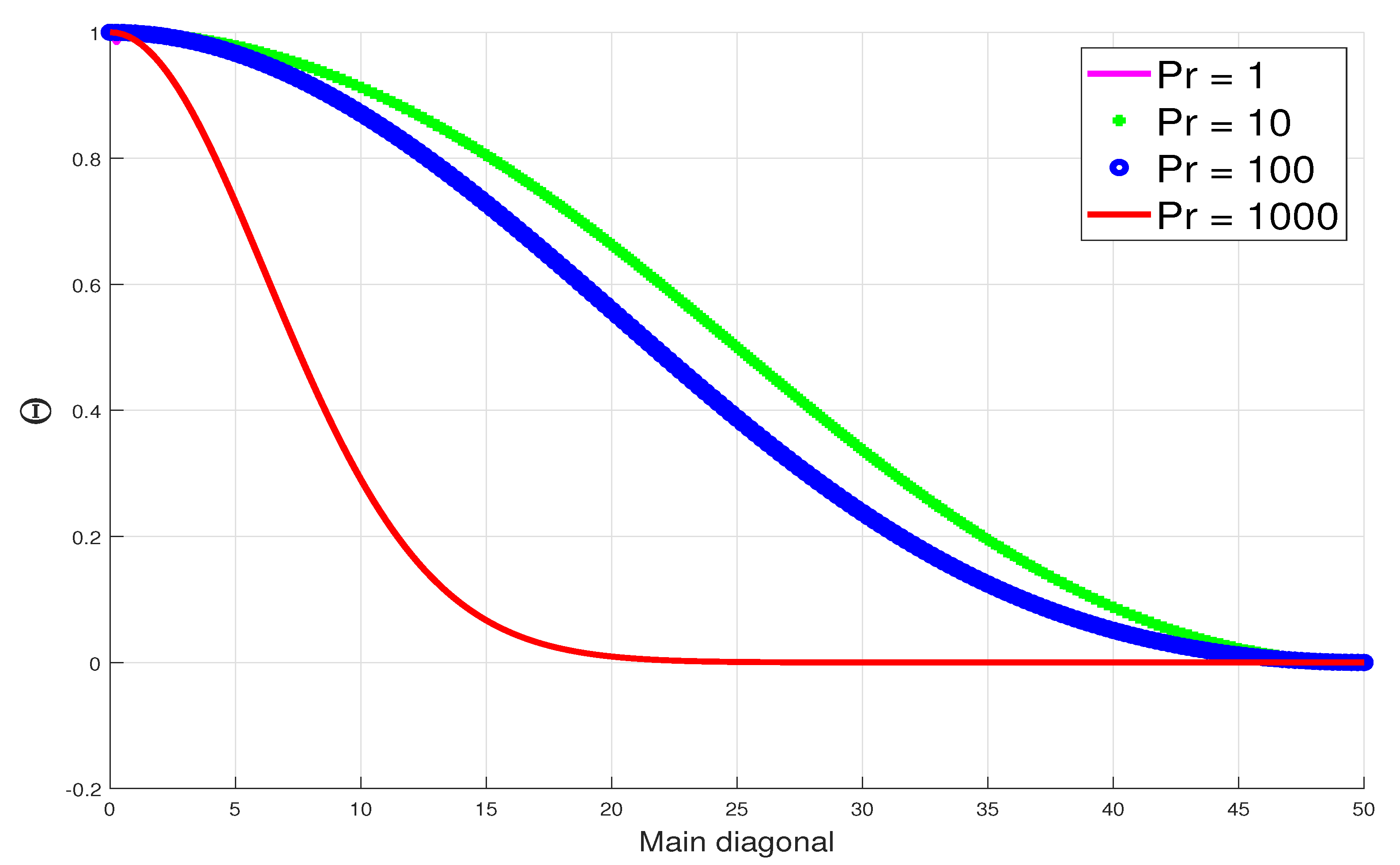
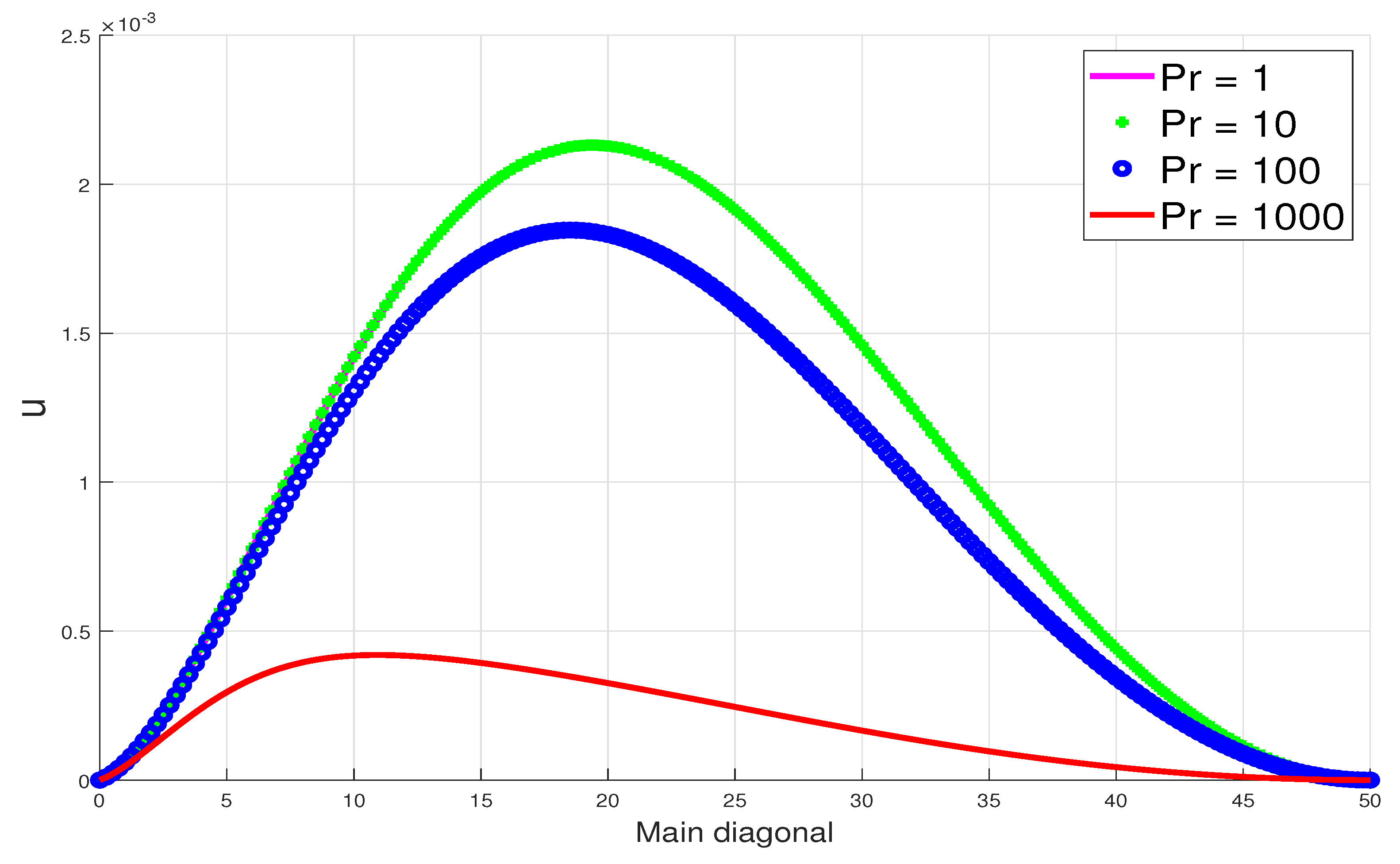
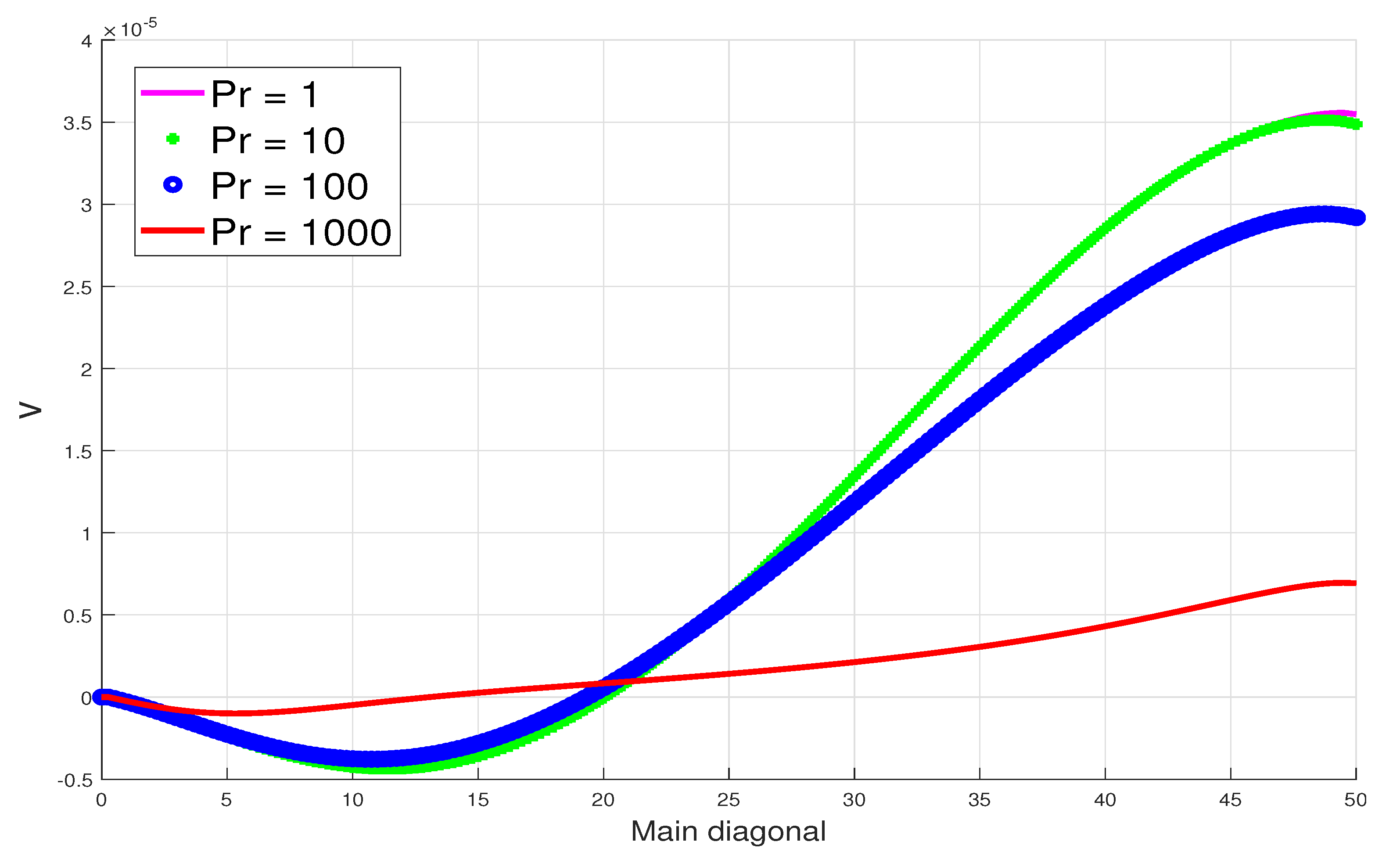
6.4. Dependence on Prandtl Number, $P$

The dependence of solutions on the Prandtl number $\mathrm{Pr}$ is illustrated in Figure 22, Figure 23 and Figure 24. Unlike the Grashof number, the Prandtl number represents the driving force for the fluid temperature. In particular, higher Prandtl number values lead to lower fluid temperatures and vice versa, as illustrated in Figure 22. Given that the fluid velocity, in the setting of natural convection flow, is directly influenced by the prevailing temperature conditions, the behaviour of the fluid velocity, therefore, mirrors that of the temperature as shown in Figure 23 and Figure 24.

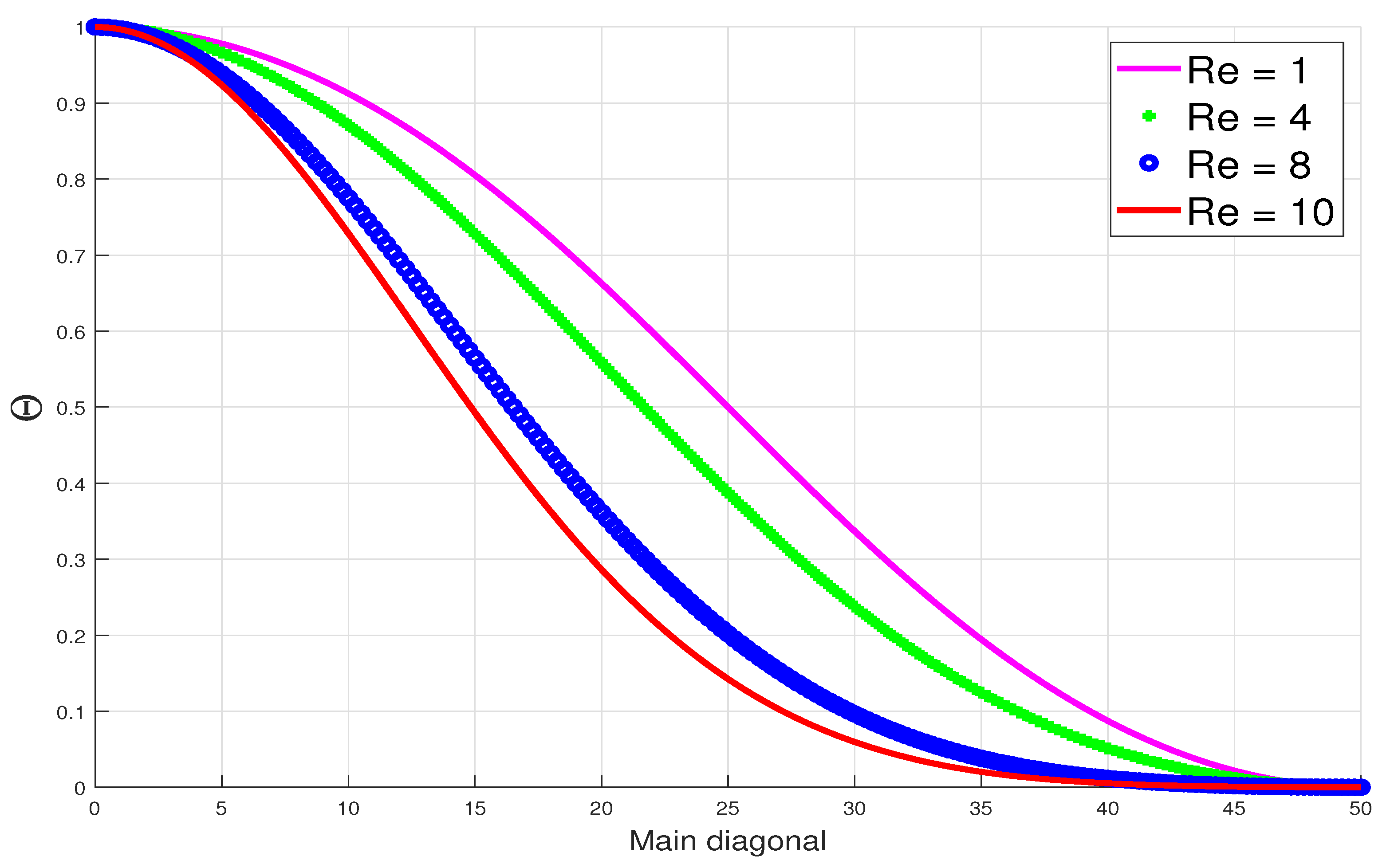
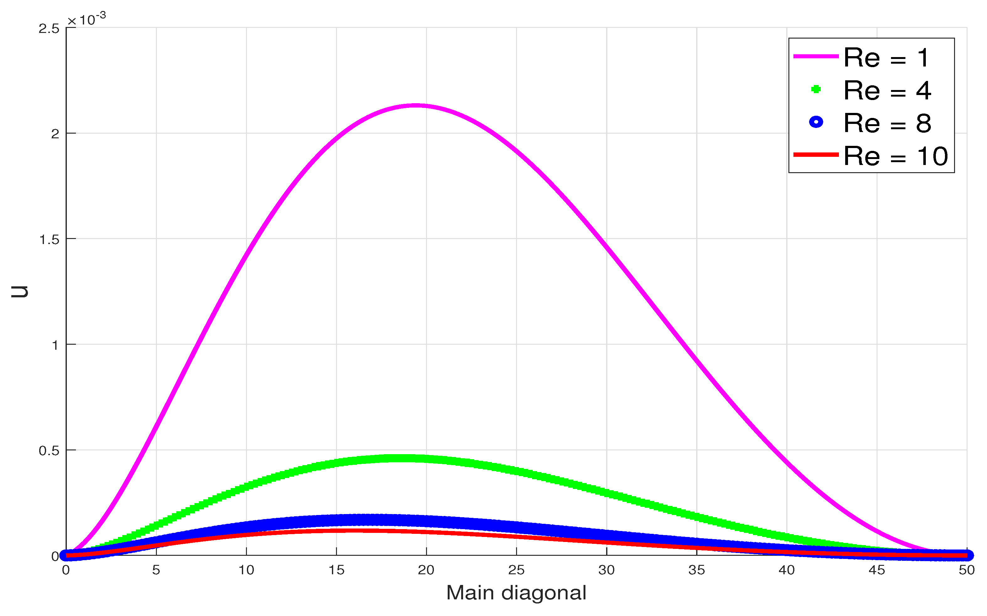
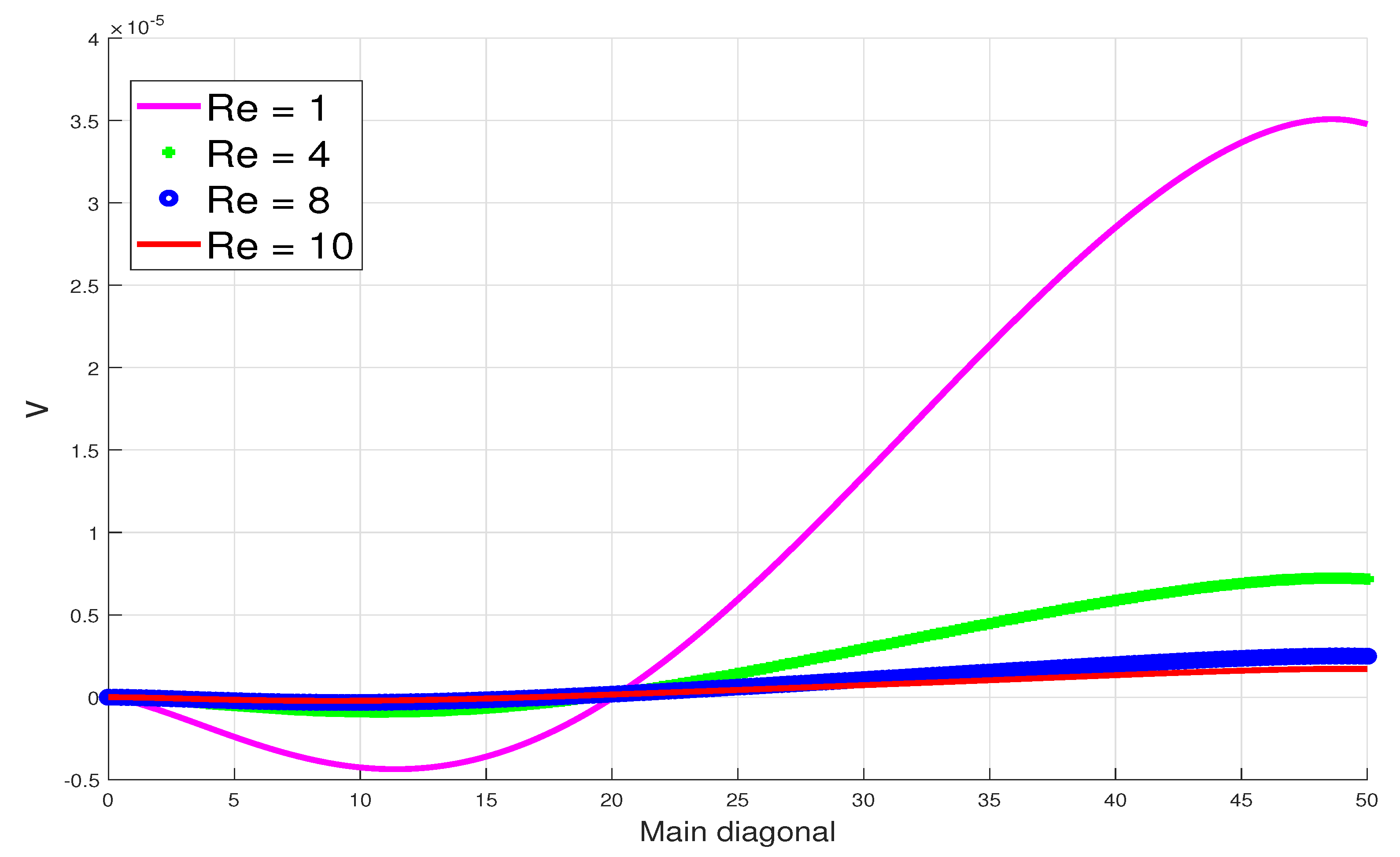
6.5. Dependence on Reynolds number, $R$

The dependence of solutions on the Reynolds number $\mathrm{Re}$ is illustrated in Figure 25, Figure 26 and Figure 27. The Reynolds number plays significant roles in the source terms of both the fluid velocity and fluid temperature. In the fluid velocity, the Reynolds number plays an inverse role to that of the Grashof number and hence increased Reynolds number leads to lower fluid velocities and vice versa. this is illustrated in Figure 26 and Figure 27. In the fluid temperature, the Reynolds number plays a similar role to that of the Prandtl number and hence increased Reynolds number leads to lower fluid temperature and vice versa, see Figure 25.

7. Conclusions

We successfully investigated, numerically, a nonlinear boundary value problem (BVP) that models the natural convection flow and heat transfer to a non-Newtonian pseudoplastic fluid in a long thin channel by recasting the BVP as an initial boundary value problem (IBVP). Our numerical algorithms are based on efficient and convergent semi-implicit time-space finite difference methods. The fluid temperature and velocities develop in time, from the zero initial conditions inside the channel until steady states are reached. At a steady state, the solutions both increase or decrease with decreasing (respectively increasing) Prandtl and/or Reynolds numbers. Changes in those flow parameters that are directly linked to the fluid velocity, such as the Grashof and viscosity parameters, are shown to have a significant effect on the fluid velocity but not on the fluid temperature.

References

1. Dumitru, V.; Constantin, F.; Nehad, A.S.; Se-Jin, Y. Unsteady natural convection flow due to fractional thermal transport and symmetric heat source/sink. Alex. Eng. J. 2023, 64, 761–770. [Google Scholar]
2. Bilal, S.; Khan, N.Z.; Shah, I.A.; Awrejcewicz, J.; Akul, A.; Riaz, M.B. Numerical Study of Natural Convection of Power Law Fluid in a Square Cavity Fitted with a Uniformly Heated T-Fin. Mathematics 2022, 10, 342. [Google Scholar] [CrossRef]
3. Nemati, H.; Moradaghay, M.; Shekoohi, S.A.; Moghimi, M.A.; Meyer, J.P. Natural convection heat transfer from horizontal annular finned tubes based on modified Rayleigh Number. Int. Commun. Heat Mass Transf. 2020, 110, 104370. [Google Scholar] [CrossRef]
4. El Moutaouakil, L.; Boukendil, M.; Zrikem, Z.; Abdelbaki, A. Natural Convection and Surface Radiation Heat Transfer in a Square Cavity with an Inner Wavy Body. Int. J. Thermophys. 2020, 41, 109. [Google Scholar] [CrossRef]
5. Alhashash, A. Natural convection of Nanoliquid from a Cylinder in Square Porous Enclosure using Buongiorno’s Two-phase Model. Sci. Rep. 2020, 10, 143. [Google Scholar] [CrossRef] [Green Version]
6. Mao, X.; Xia, H. Natural Convection Heat Transfer of the Horizontal Rod-Bundle in a Semi-closed Rectangular Cavity. Front. Energy Res. 2020, 8, 74. [Google Scholar] [CrossRef]
7. Begum, N.; Siddiqa, S.; Ouazzi, A.; Hossain, M.A.; Gorla, R.S.R. Natural Convection and Separation Points of a Non-Newtonian Fluid Along a Rotating Round-Nosed Body. J. Thermophys. Heat Transf. 2018, 32, 946–952. [Google Scholar] [CrossRef]
8. Siddiqa, S.; Begum, N.; Hossain, M.A.; Gorla, R.S.R.; Al-Rashed, A.A. Two-phase natural convection dusty nanofluid flow. Int. J. Heat Mass Transf. 2018, 118, 66–74. [Google Scholar] [CrossRef]
9. Abu-Libdeh, N.; Redouane, F.; Aissa, A.; Mebarek-Oudina, F.; Almuhtady, A.; Jamshed, W.; Al-Kouz, W. Hydrothermal and Entropy Investigation of Ag/MgO/H2O Hybrid Nanofluid Natural Convection in a Novel Shape of Porous Cavity. Appl. Sci. 2021, 11, 1722. [Google Scholar] [CrossRef]
10. Lai, T.; Xu, J.; Liu, X.; He, M. Study of Rotation Effect on Nanofluid Natural Convection and Heat Transfer by the Immersed Boundary-Lattice Boltzmann Method. Energies 2022, 15, 9019. [Google Scholar] [CrossRef]
11. Hua, Y.; Peng, J.-Z.; Zhou, Z.-F.; Wu, W.-T.; He, Y.; Massoudi, M. Thermal Performance in Convection Flow of Nanofluids Using a Deep Convolutional Neural Network. Energies 2022, 15, 8195. [Google Scholar] [CrossRef]
12. Mahdy, A.; El-Zahar, E.R.; Rashad, A.M.; Saad, W.; Al-Juaydi, H.S. The Magneto-Natural Convection Flow of a Micropolar Hybrid Nanofluid over a Vertical Plate Saturated in a Porous Medium. Fluids 2021, 6, 202. [Google Scholar] [CrossRef]
13. Baliti, J.; Elguennouni, Y.; Hssikou, M.; Alaoui, M. Simulation of Natural Convection by Multirelaxation Time Lattice Boltzmann Method in a Triangular Enclosure. Fluids 2022, 7, 74. [Google Scholar] [CrossRef]
14. Gibanov, N.S.; Sheremet, M.A. Numerical Investigation of Conjugate Natural Convection in a Cavity with a Local Heater by the Lattice Boltzmann Method. Fluids 2021, 6, 316. [Google Scholar] [CrossRef]
15. Huang, J.S. Numerical Study of Thermophoresis on Mass Transfer from Natural Convection Flow over a Vertical Porous Medium with Variable Wall Heat Fluxes. Appl. Sci. 2021, 11, 10418. [Google Scholar] [CrossRef]
16. Quintino, A.; Cianfrini, M.; Petracci, I.; Spena, V.A.; Corcione, M. Dimensionless Correlations for Natural Convection Heat Transfer from a Pair of Vertical Staggered Plates Suspended in Free Air. Appl. Sci. 2021, 11, 6511. [Google Scholar] [CrossRef]
17. Ishigaki, M.; Hirose, Y.; Abe, S.; Nagai, T.; Watanabe, T. Estimation of Flow Field in Natural Convection with Density Stratification by Local Ensemble Transform Kalman Filter. Fluids 2022, 7, 237. [Google Scholar] [CrossRef]
18. Zhang, Y.; Yang, X.; Zhang, L.; Li, Y.; Zhang, T.; Sun, S. Energy landscape analysis for two-phase multi-component NVT flash systems by using ETD type high-index saddle dynamics. J. Comput. Phys. 2023, 477, 111916. [Google Scholar] [CrossRef]
19. Zhang, T.; Zhang, Y.; Katterbauer, K.; Al Shehri, A.; Sun, S.; Hoteit, I. Phase equilibrium in the hydrogen energy chain. Fuel 2022, 328, 125324. [Google Scholar] [CrossRef]
20. Bondareva, N.S.; Sheremet, M.A. Natural Convection Melting Influence on the Thermal Resistance of a Brick Partially Filled with Phase Change Material. Fluids 2021, 6, 258. [Google Scholar] [CrossRef]
21. Chinyoka, T. Two-dimensional flow of chemically reactive viscoelastic fluids with or without the influence of thermal convection. Commun. Nonlinear Sci. Numer. Simul. 2011, 16, 1387–1395. [Google Scholar] [CrossRef]
22. Chinyoka, T. Viscoelastic effects in double-pipe single-pass counterflow heat exchangers. Int. J. Numer. Methods Fluids 2009, 59, 677–690. [Google Scholar] [CrossRef]
23. Chinyoka, T. Modeling of cross-flow heat exchangers with viscoelastic fluids. Nonlinear Analysis: Real World Appl. 2009, 10, 353–3359. [Google Scholar] [CrossRef]
24. Mavi, A.; Chinyoka, T.; Gill, A. Modelling and Analysis of Viscoelastic and Nanofluid Effects on the Heat Transfer Characteristics in a Double-Pipe Counter-Flow Heat Exchanger. Appl. Sci. 2022, 12, 5475. [Google Scholar] [CrossRef]
25. Mavi, A.; Chinyoka, T. Volume-of-Fluid Based Finite-Volume Computational Simulations of Three-Phase Nanoparticle-Liquid-Gas Boiling Problems in Vertical Rectangular Channels. Energies 2022, 15, 5746. [Google Scholar] [CrossRef]
26. Khan, I.; Chinyoka, T.; Gill, A. Computational Analysis of Shear Banding in Simple Shear Flow of Viscoelastic Fluid-Based Nanofluids Subject to Exothermic Reactions. Energies 2022, 15, 1719. [Google Scholar] [CrossRef]
27. Khan, I.; Chinyoka, T.; Gill, A. Computational Analysis of the Dynamics of Generalized-Viscoelastic-Fluid-Based Nanofluids Subject to Exothermic-Reaction in Shear-Flow. J. Nanofluids 2022, 11, 487–499. [Google Scholar] [CrossRef]
28. Khan, I.; Chinyoka, T.; Gill, A. Dynamics of Non-Isothermal Pressure-Driven Flow of Generalized Viscoelastic-Fluid-Based Nanofluids in a Channel. Math. Probl. Eng. 2022, 2022, 9080009. [Google Scholar] [CrossRef]
29. Cross, M.M. Rheoogy of non-Newtonian fluids: A new flow equation for pseudoplastic systems. J. Colloid Sci. 1965, 20, 417–437. [Google Scholar] [CrossRef]
30. Xie, J.; Jin, Y. Parameter determination for the Cross rheology equation and its application to modeling non-Newtonian flows using the WC-MPS method. Eng. Appl. Comput. Fluid Mech. 2016, 10, 111–129. [Google Scholar] [CrossRef] [Green Version]
Figure 1. Schematic of the model.
Applsci 13 03224 g001
Figure 2. Illustration of mesh size independence at mid-point of the domain and t = 5 .
Applsci 13 03224 g002
Figure 3. Illustration of time-step size independence at mid-point of the domain and t = 5 .
Applsci 13 03224 g003
Figure 4. Time development of steady-state temperature profiles.
Applsci 13 03224 g004
Figure 5. Time development of steady-state axial velocity profiles.
Applsci 13 03224 g005
Figure 6. Time development of steady-state transverse velocity profiles.
Applsci 13 03224 g006
Figure 7. Surface plot of the temperature profile at t = 10 .
Applsci 13 03224 g007
Figure 8. Contour plot of the temperature profile at t = 10 .
Applsci 13 03224 g008
Figure 9. Surface plot of the u-velocity profile at t = 10 .
Applsci 13 03224 g009
Figure 10. Contour plot of the u-velocity profile at t = 10 .
Applsci 13 03224 g010
Figure 11. Surface plot of the v-velocity profile at t = 10 .
Applsci 13 03224 g011
Figure 12. Contour plot of the v-velocity profile at t = 10 .
Applsci 13 03224 g012
Figure 13. Temperature dependence on n at t = 5 .
Applsci 13 03224 g013
Figure 14. Axial velocity dependence on n at t = 5 .
Applsci 13 03224 g014
Figure 15. Transverse velocity dependence on n at t = 5 .
Applsci 13 03224 g015
Figure 16. Temperature dependence on α at t = 5 .
Applsci 13 03224 g016
Figure 17. Axial velocity dependence on α at t = 5 .
Applsci 13 03224 g017
Figure 18. Transverse velocity dependence on α at t = 5 .
Applsci 13 03224 g018
Figure 19. Temperature dependence on Gr at t = 5 .
Applsci 13 03224 g019
Figure 20. Axial velocity dependence on Gr at t = 5 .
Applsci 13 03224 g020
Figure 21. Transverse velocity dependence on Gr at t = 5 .
Applsci 13 03224 g021
Figure 22. Temperature dependence on Pr at t = 5 .
Applsci 13 03224 g022
Figure 23. Axial velocity dependence on Pr at t = 5 .
Applsci 13 03224 g023
Figure 24. Transverse velocity dependence on Pr at t = 5 .
Applsci 13 03224 g024
Figure 25. Temperature dependence on Re at t = 5 .
Applsci 13 03224 g025
Figure 26. Axial velocity dependence on Re at t = 5 .
Applsci 13 03224 g026
Figure 27. Transverse velocity dependence on Re at t = 5 .
Applsci 13 03224 g027
Disclaimer/Publisher’s Note: The statements, opinions and data contained in all publications are solely those of the individual author(s) and contributor(s) and not of MDPI and/or the editor(s). MDPI and/or the editor(s) disclaim responsibility for any injury to people or property resulting from any ideas, methods, instructions or products referred to in the content.