Differential Evolution Applied to a Multilevel Inverter—A Case Study

Abstract

This work aims to obtain the switching angles to reduce the total harmonic distortion (THD) and compare the different sets of angles obtained by modifying the modular index (Mi) in a seven-level multilevel inverter using the differential evolution (DE) algorithm. A seven-level cascaded multilevel inverter with RL load was simulated in MATLAB Simulink. The Mi was varied (0.6 to 1.27) to check which set of switching angles is optimal to reduce the THD. These sets of angles are then experimentally validated on a test bench. A brief discussion of the results is presented, comparing the minimum THD found without considering Mi, versus the minimum THD obtained if Mi is less than 1.

1. Introduction

Metaheuristic algorithms are optimization algorithms attempt to improve the search for solutions in the search space iteratively. The algorithms may be inspired by biological phenomena or by the social behavior of species. Metaheuristic algorithms are usually problem-independent. Due to their specific advantages over classical methods, metaheuristics are used in the solution of different problems in the fields of engineering [1].

Among the metaheuristic methods that have been used for the solution of these problems are differential evolution, particle optimization (PSO), genetic algorithm (GA), firefly algorithm (FA), and others. However, the differential evolution algorithm has distinguished itself for its efficiency and belongs to the evolutionary algorithms. Among the outstanding features of the differential evolution algorithm are its efficient global search capability, versatility to the characteristics of the problem, and not requiring a suitable initial solution [2].

Differential evolution has been used in various engineering fields, such as acoustics, aerodynamics, aerospace, agriculture, automotive, biology, chemistry, defense, and others. The differential evolution algorithm has been widely used in electricals and electronics, in various communication systems (multi-input and multi-output systems), power allocation, system modeling, controller design for complex dynamic systems, radio network design, ultra-wideband radio systems, and power converters [3].

Multilevel inverters (MLIs) can create a single output waveform by synthesizing multiple voltage levels, producing a stepped waveform approximating a sinusoidal signal. As the number of sources at the input to the inverter increases, so does the number of levels of the output waveform [4,5]. Due to the stepped nature of the multilevel inverter output waveform, multiple sets of switching angles can be found for one modulation index (Mi) value [6].

For applications related to power converters, the differential evolution algorithm has been used to minimize THD in multilevel inverters by calculating the optimal switching angles.

The solution of the transcendental nonlinear equations is one of the main problems in calculating the optimal switching angles to minimize THD. Therefore, different optimization methods have been used in the literature to eliminate harmonics by solving the nonlinear transcendental equations that generate the Fourier series.

Several papers mention performing a sweep of the Mi and obtaining results of a minimum THD using a Mi > 1 [6,7,8], which can produce an overmodulation, and they only considered using the minimum %THD found. In other papers [9,10,11,12], “coincidentally”, the minimum %THD found had a Mi > 0.6 and <1. Reviewing the angles found in these papers that coincide in the number of levels (7), they obtain a set of switching angles different from each other. Additionally, other articles do not mention which Mi they used. Moreover, they have different levels, loads, and phases implemented in the MLIs.

This paper focuses on the differential evolution (DE) algorithm application to minimize the THD value in the output voltage waveform of a cascaded multilevel inverter and to analyze the obtained sets of switching angles calculated to achieve a required modular index according to the inverter application.

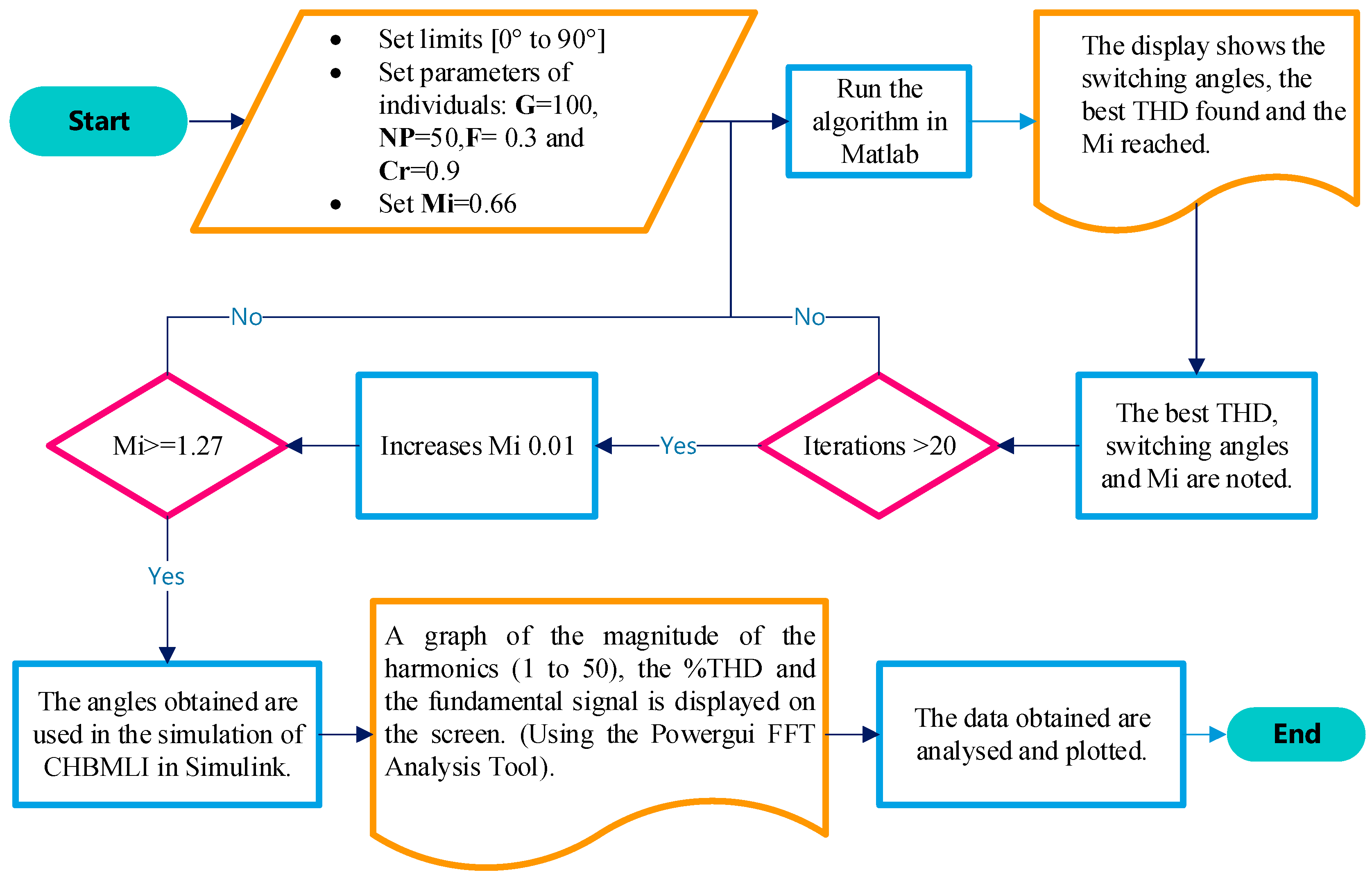
2. Materials and Methods

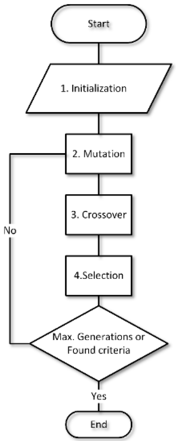
2.1. Differential Evolution Algorithm

The differential evolution (DE) algorithm is a relatively new metaheuristic method. The DE algorithm is a population-based algorithm that uses genetic operators such as crossover, mutation, and selection.

It has become one of the most widely used evolutionary algorithms. It is easily understood and easy to implement.

Kenneth and Storn developed the differential evolution algorithm as a reliable, versatile, easy-to-implement function optimizer. The first publication on DE appeared in a technical report in 1995 [13].

This metaheuristic method has three principal operations: mutation, crossover, and selection. In the mutation stage, the population vectors are randomly perturbed. Population diversity is controlled by the crossover process [14]. Meanwhile, the selection process chooses the vectors containing the fittest solution [15].

Some advantages of the DE method are its ease of application, fast convergence, and tendency to reach the global optimal solution without remaining in local solutions [16,17]. A diagram of the stages of DE is shown in Figure 1.

The following is a brief description of each stage outlined in the diagram in Figure 1:

• Initialization (Initial population): A population of vectors is randomly generated (individuals) [18,19,20].

$$\mathrm{Let} S^G=\{X_j^G:j=1,2,\dots ,NP\}$$

(1)

be the population of any generation of G, NP denotes the population size. D is the length of the search space.

$$X_j^G=\left\{x_{1,j}^{G }, x_{2,j}^{G }, \dots , x_{D,j}^G\right\}· X_j^G$$

(2)

is generated using a uniformly distributed random number, such as: “rand (0,1)”. Hence, we obtain:

$$X_j^G=X_{Low}+\left.\left(X_{Upp}-X_{Low}\right.\right)\ast rand\left.\left(0,1\right.\right)$$

(3)

where:

X_Low = Lower bound.

X_Upp = Upper bound.

S^G = search space.

2.

Mutation: In this process, three vectors are randomly selected, and the first two vectors are subtracted from each other (this is to define a search direction). The difference is multiplied by the scale factor or “F”, which can vary between zero and one [12]. To the resulting vector, the third vector is added [21], as in the following equation:

$$V_j^G=X_{r3}^G+F\ast \left.\left(X_{r1}^G-X_{r2}^G\right.\right)$$

(4)

where V_j^G is the mutant vector.

For each vector in the population, a mutated vector is created.

3.

Crossover: A new vector called the test vector (child vector) is generated, using a crossover factor Cr with values between 0 and 1 and defining the degree of similarity of the test vector to the mutant or parent vector. If Cr is close to 1, the test vector will be quite similar to the mutant vector; if Cr is close to 0, it will be similar to the parent vector [19,20].

The test vector U_j^G, the target vector X_j^G, and the mutant vector V_j^G are denoted as:

$$U_j^G=\{u_{1,j}^G, u_{2,j}^G, \dots , u_{D,j}^G\}$$

$$X_j^G=\{x_{1,j}^G, x_{2,j}^G, \dots , x_{D,j}^G\}$$

$$V_j^G=\{v_{1,j}^G, v_{2,j}^G, \dots , v_{D,j}^G\}$$

so U_j^G is generated as:

$$u_{i,j}^G=\left\{\begin{array}{c}{v}_{i,j }^{G}If ran{d}_j\le Cr\\ x_{i,j}^G Otherwise\end{array}\right.$$

(5)

where i ∈ {1, 2,…, D}.

4.

Selection: The target vector is compared with the test vector. The vector with the highest fitness remains in the next generation, while the vector with the lowest fitness is eliminated [3,20]. This operation is performed as:

$$X_j^{G+1}=\left\{\begin{array}{c}{U}_{j }^{G}If f\left(U_{j }^G\right)\le f\left(U_{j }^G\right)\\ X_j^G Otherwise\end{array}\right.$$

(6)

Scale factor (F) influences the search’s orientation and convergence speed. If the F factor takes values between 0.1 and 0.4, it allows a better local search in the space. If F takes a value between 0.4 and 0.95, the algorithm performs a better global search. Some authors recommend using 0.9, as it maintains a balance between speed and probability of convergence [15,22,23].

Several authors recommend using a crossover rate (Cr) with a value of 0.9 so that the test vector will be 90% similar to the mutant vector and thus include a wide variety of individuals [24].

2.2. Optimization Problem Statement

Optimization is obtaining the best possible solution to several designs and engineering problems.

An optimization problem contains three important aspects:

• Objective function: the property to be optimized, which can be expressed as a linear or non-linear function.
• Decision variable: an unknown element of an optimization problem.
• Constraints: restrictions that must be satisfied to produce an acceptable result.

For a stated objective function that is defined on the set of all decision variables, a decision must be found such that the objective is optimized (minimized or maximized) [1,25].

An optimization problem may be as follows:

$$\min f\left(x\right) ,subject to x \in \Omega$$

(7)

where “f” is a real-valued function called the objective function.

The vector “x” is a vector of “n” independent variables x = [x₁, x₂… x_n] where the variables x₁, x₂… x_n, often referred to as decision variables, are selected by the user or designer. The set Ω is a subset of R called the constraint set or feasible set.

The above problem is a decision problem. It involves finding the “best” vector x in compliance with the constraints, or nay, all possible vectors within Ω. The “best” vector is the one that has the smallest value of the objective function. This vector is called the “minimizer”. It is possible to have many minimizers.

Most engineering problems require the designer to optimize some conflicting objectives. Objectives conflict if one objective’s improvement leads to another’s deterioration. The simplest way to optimize is to find a decision variable that satisfies the given constraints and optimizes a function whose components are objective functions [25,26]. Multi-objective problems may not have a single optimal solution.

In this paper, the optimization problem is the reduction of THD in a cascade H-bridge multilevel inverter (CHBMLI) and finding a desired value of Mi according to the application. Starting from the THD, the stepped waveform of the output voltage is analyzed using the Fourier series and is expressed in the following equation, considering that it has quarter-wave symmetry:

$$V_{\mathit{out}}(\theta ) = {{\displaystyle \sum }}_{n=1,3,5}^{\infty }{b}_n sin\left(n\theta \right)$$

(8)

where n = 1, 3, 5 are odd harmonics, and b_n is given by:

$$b_n={{\displaystyle \sum }}_{n=1,3,5}^{2N-1}\frac{4V_{dc}}{n\pi }\left(V_1\cos \left(n{\alpha }_1\right)+V_2\cos \left(n{\alpha }_2\right)+\cdots V_m\cos \left(n{a}_N\right)\right)$$

(9)

where:

N = number of switching angles per quarter cycle.

n = 1, 3, 5… 2N−1 (odd harmonics).

m = number of DC sources.

α = switching angle.

The quality of the output voltage waveform is determined by how many harmonics it contains, so Equation (4) shows the THD formula following the IEEE 519 standard to be set as an objective function:

$$THD=\frac{\sqrt{{{\displaystyle \sum }}_{n=1,3,5,7\dots }^{50}{V}_n^2}}{V_1}\ast 100$$

(10)

where:

$$V=\frac{4V_{dc}}{n\pi } \cos \left(n{\alpha }_1\right) + \frac{4V_{dc}}{n\pi } \cos \left(n{\alpha }_2\right) + \dots \frac{4V_{dc}}{n\pi } \cos \left(n{\alpha }_n\right),$$

The angles must satisfy the following constraints:

$$0\le {\alpha }_1\le {\alpha }_2\dots \le {\alpha }_n\le \frac{\pi }{2}$$

(11)

where n = number of switching angles per quarter cycle and α₁ = switching angle 1, α₂ = switching angle 2, and α_n = switching angle n (The switching angles are the decision variables).

When Mi > 1, it is said that there is over-modulation, which results in the absence of pulses when comparing the modulating signal with the carrier signal.

Regarding Mi, the modulation ratio is equal to V1 over n.

Recalling that the case study is a seven-level CHBMLI, Figure 2 shows a waveform with seven levels and three switching angles (n = 3); the equation remains:

$$Mi=\frac{4}{3\pi }\left(\cos \left({\propto }_1\right)+\cos \left({\propto }_2\right)+\cos \left({\propto }_3\right)\right)$$

(12)

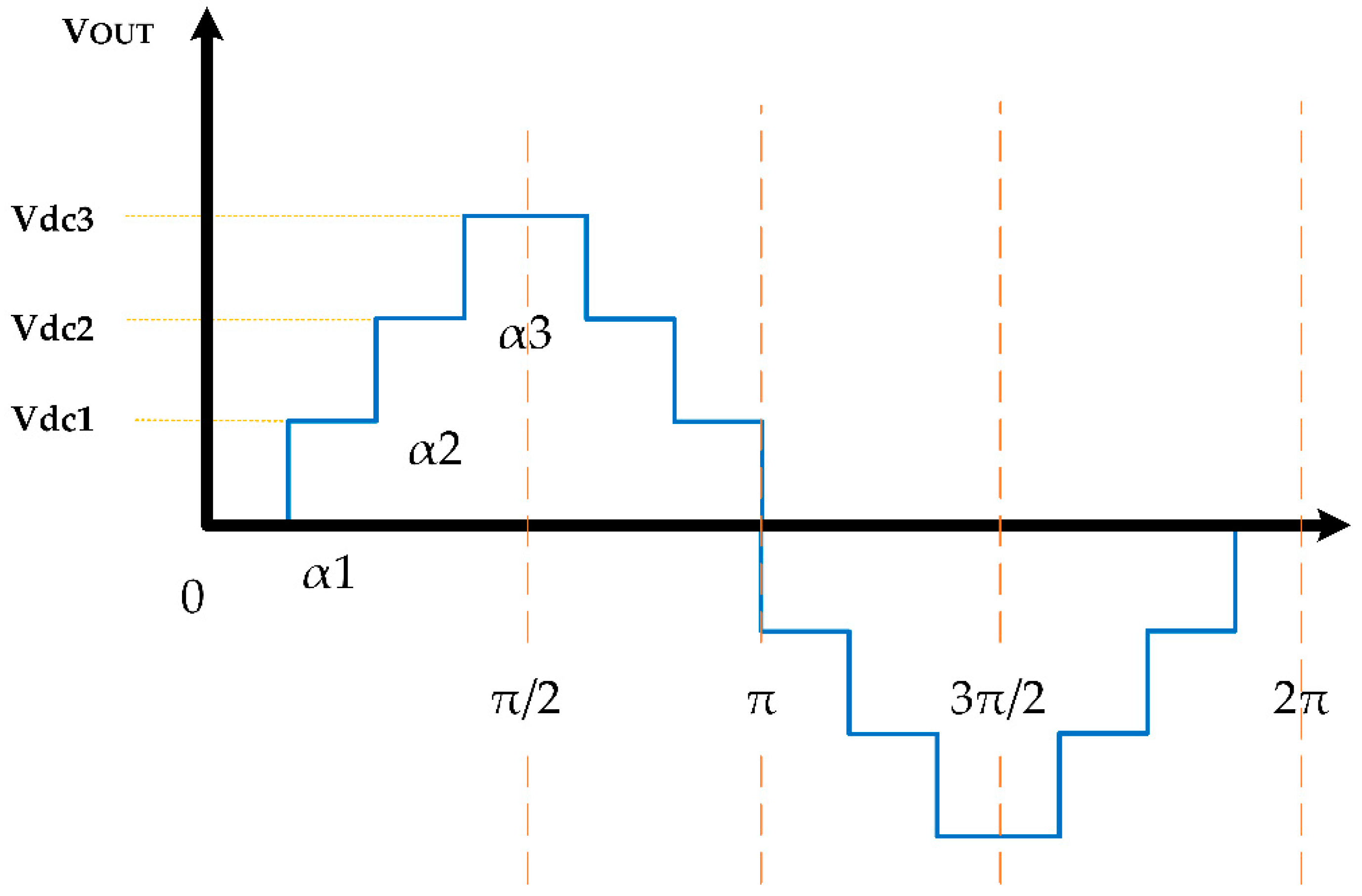
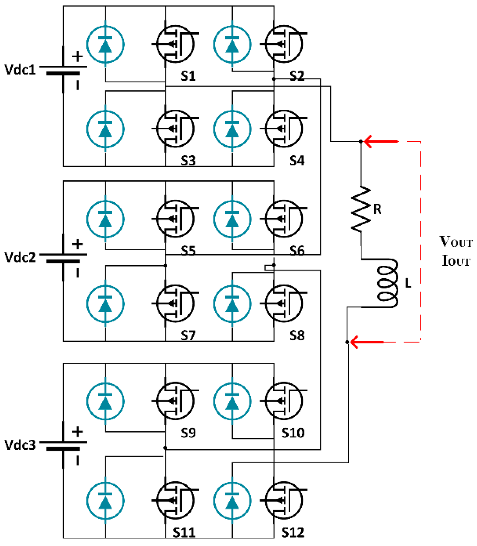
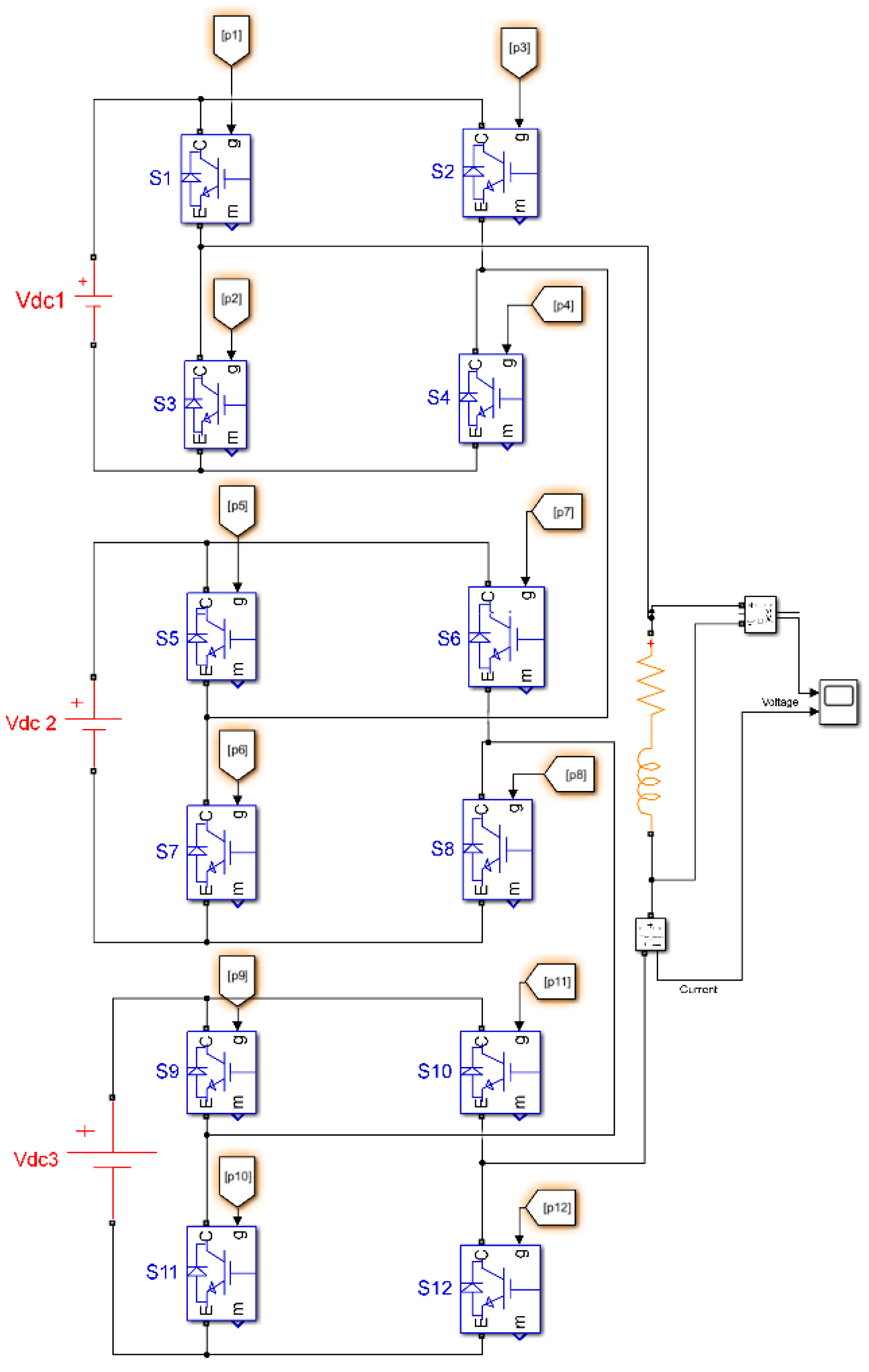
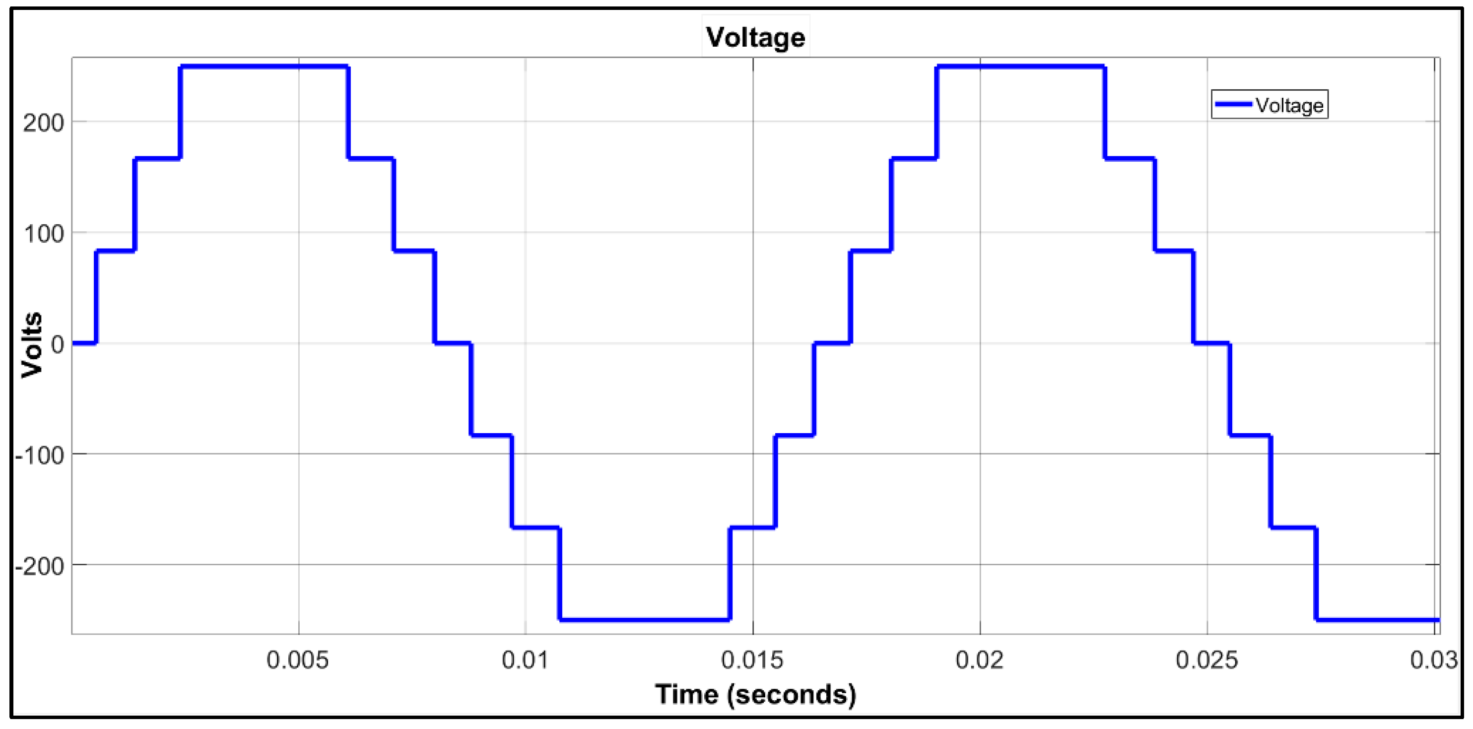
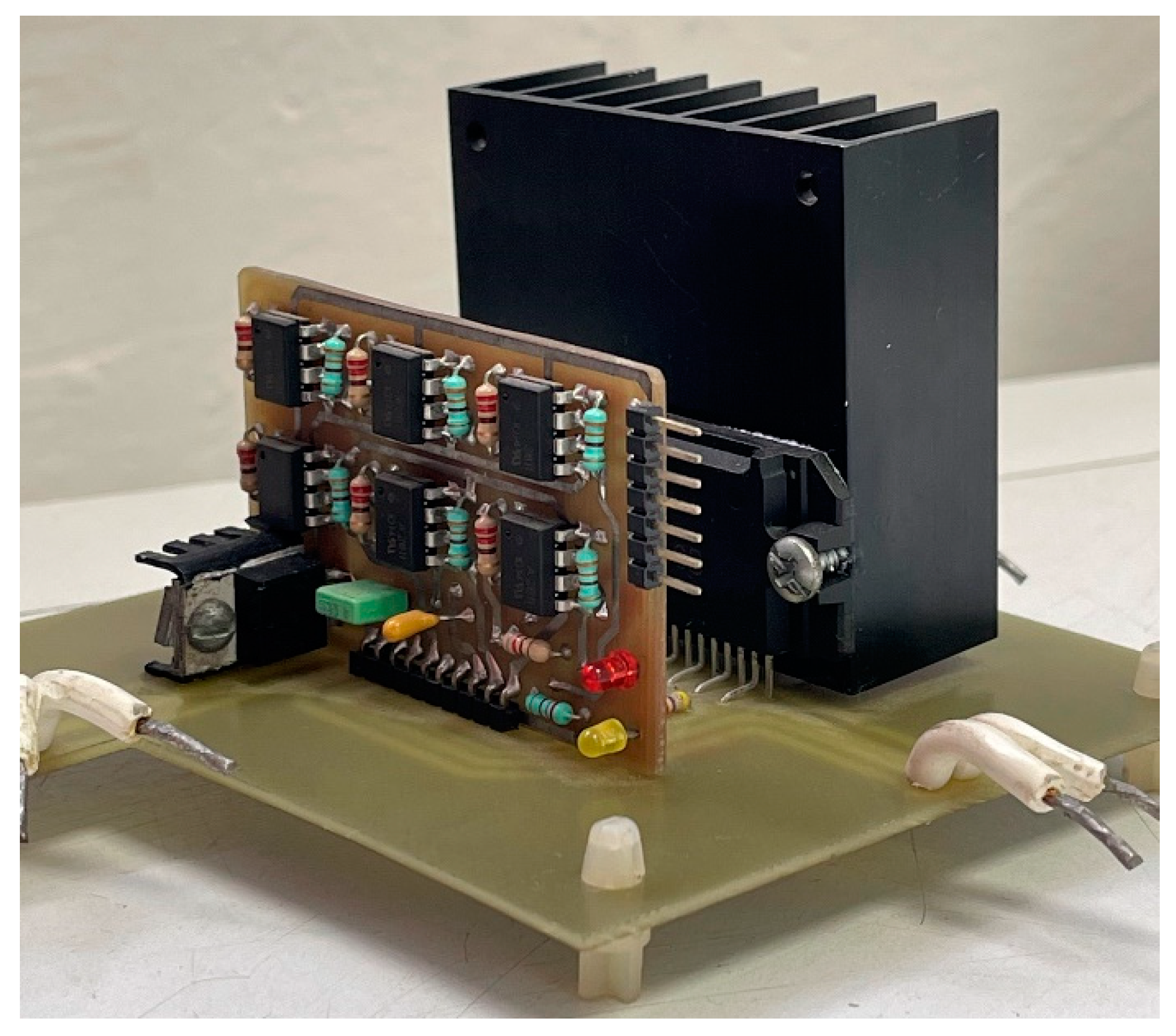
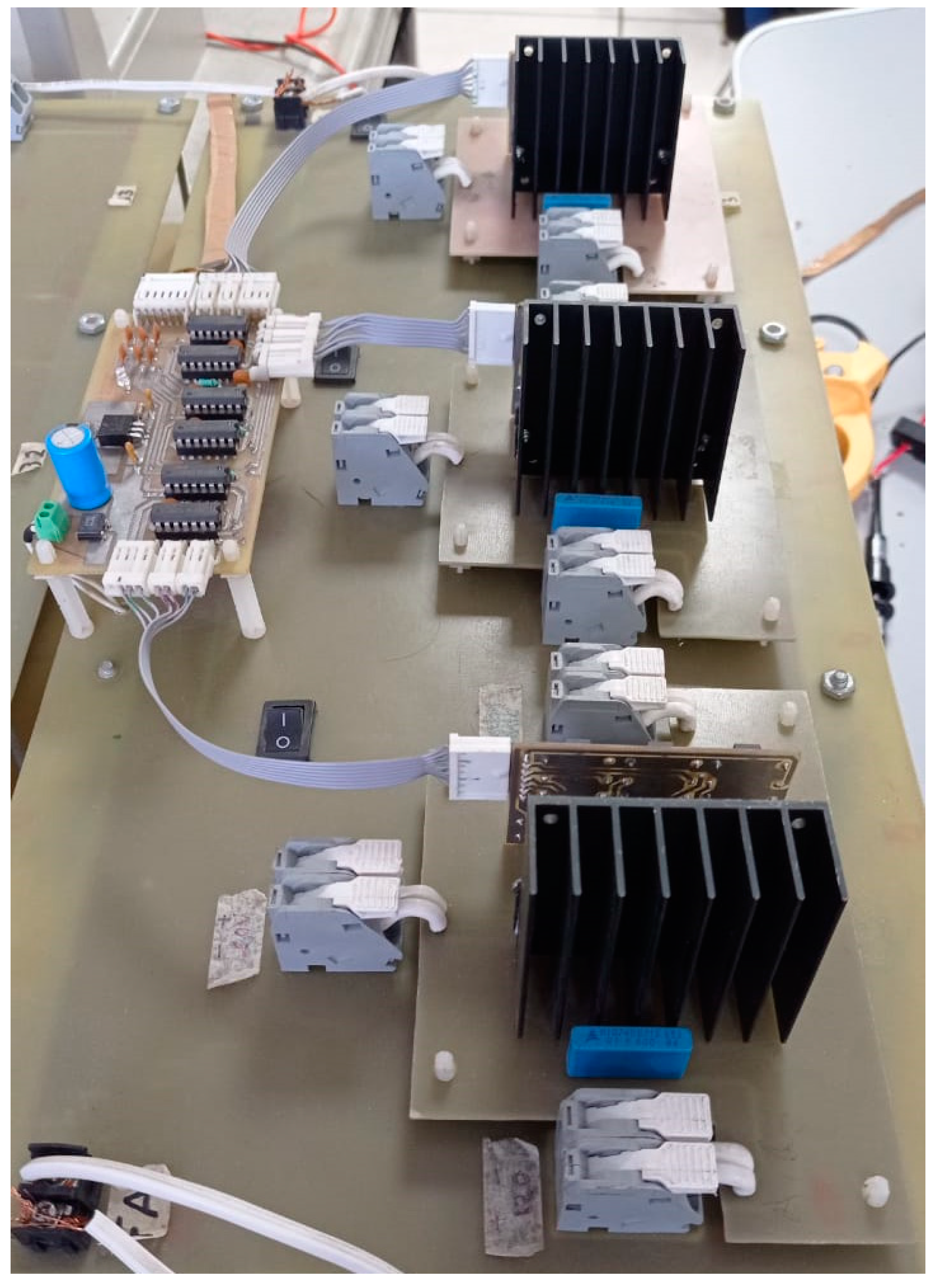
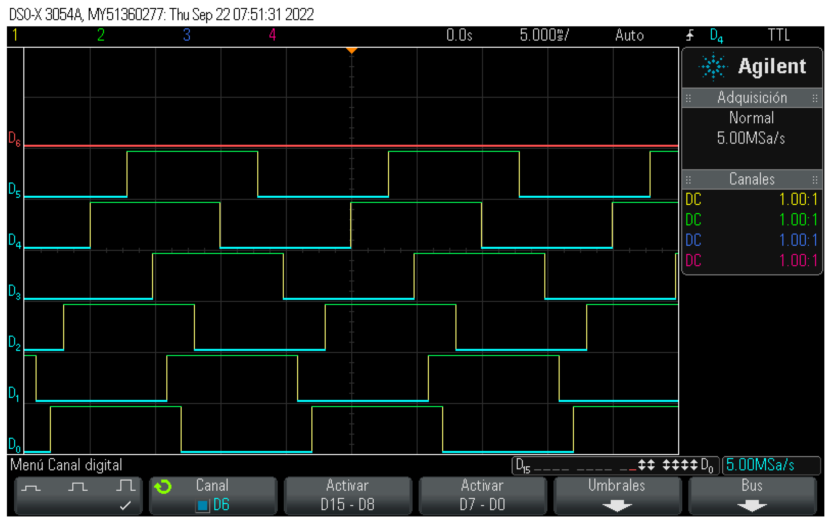
2.3. Structure of the Seven-Level Cascaded Multilevel Inverter: Case Study

Reference [27] provides a systematic review of publications using metaheuristic methods to minimize THD in multilevel inverters. The publication highlights that the most used topology in combination with the differential evolution algorithm is the single-phase cascaded multilevel inverter with seven levels.

The most outstanding features of CHBMLI are:

• The generation of its switching signals is simple, allowing the use of any PWM technique based on multi-carrier or vector spaces [28,29].
• Switching states can be changed to compensate for faults.
• Input capacitors have no voltage balance problems [30].

Considering the advantages, the topology selected as a case study for this paper is the seven-level single-phase CHBMLI with an RL load connected to the output, as shown in Figure 3. MATLAB Simulink software was used to perform the simulation of the case study. The differential evolution method is used to minimize THD.

Table 1. Most important parameters for the simulation of CHBMLI in MATLAB.

Parameters	Specifications
Voltage sources (Vdc 1,2,3)	83.33 V
R Load	100 Ω
L Load	100 mH
Power	625 W
Peak Voltage (Vout)	250 V
Frequency	60 Hz

shows the parameters used for the design and simulation of the cascaded multilevel inverter:

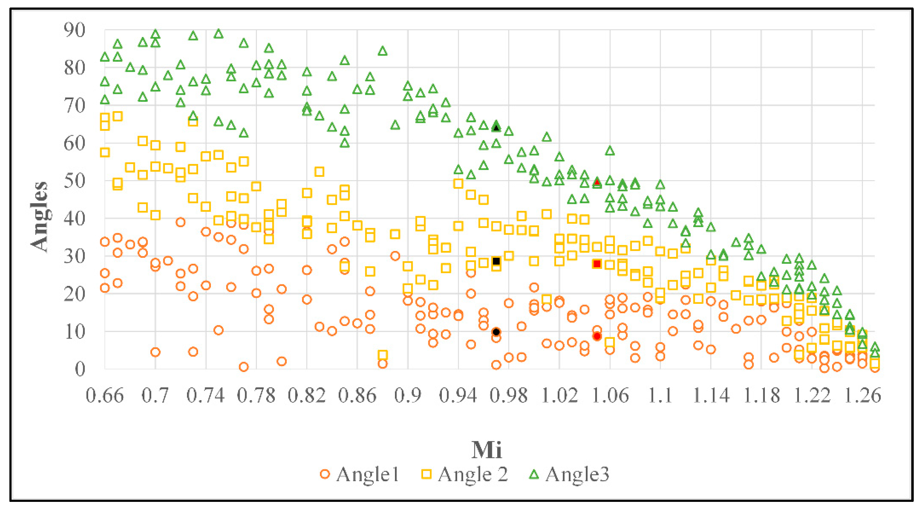
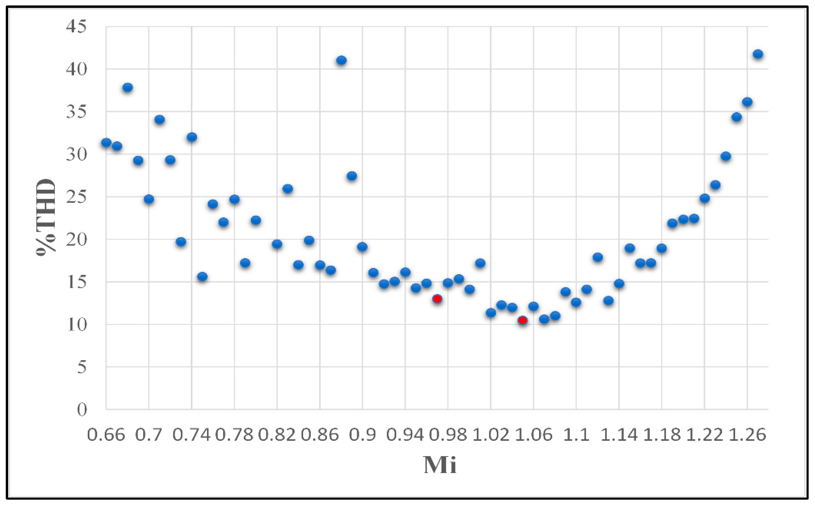
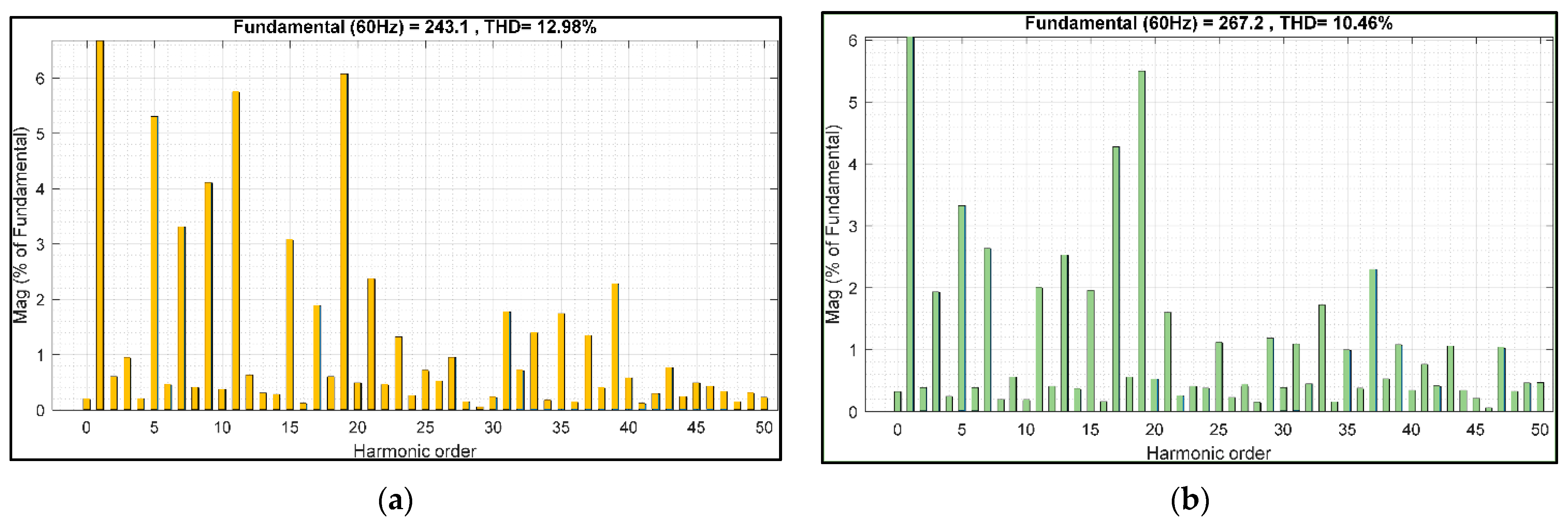
3. Simulation Results

MATLAB software was used to program the DE algorithm.

For this case study, three switching angles (∝1, ∝2, and ∝3) were searched for the seven-level CHBMLI.

After obtaining the different sets of switching angles, the modulation index sweep was performed.

Figure 4 shownn the simulation diagram of the seven-level single-phase CHBMLI, was performed in MATLAB Simulink software using the parameters in Table 1.

Figure 5 shows the output voltage waveform realized in MATLAB Simulink.

As shown in Figure 5, the output peak voltage obtained is 250 V.

The initialization parameters of the differential evolution algorithm reported in [31] were taken as a starting point. The parameters used in the case study of this article are shown in

Table 2. Parameter values for the differential evolution algorithm.

Parameter	Value
Population (NP)	100
Generation (G)	100
Scaling Factor (F)	0.3
Crossover rate (Cr)	0.9

.

Figure 6 shows the step-by-step procedure of the methodology that was carried out to obtain the different sets of angles, the Mi, and the THD percentage.

The results of the seven-level CHBMLI previously simulated in Simulink were tested and plotted to observe its behavior. The following figure shows the results of the angles obtained by the implementation of this algorithm.

Figure 7 shows the graph of the different sets of angles obtained (Angle 1 circles, Angle 2 squares, and Angle 3 triangles) that coincide with some Mi.

The set of angles depends on Mi; the smaller the Mi, the more sets are available. Two sets of angles showing the best angles (with lowest THD) found for a Mi of 0.97 (marked with black color) and 1.05 (marked with red color) have been marked in Figure 7 to generate the following Table.

In Figure 8, only the lowest THD obtained from the set of angles corresponding to each modular index was used, considering that in Figure 7, there are four combinations of angles for one Mi.

As can be seen in Figure 8, the Mi that reached the minimum percentage of THD was 1.05 (10.46%).

Several articles do not consider the value of Mi; there is a probability of not finding the optimal angles to reduce the THD or generate an overmodulation. For this case study, the values with a Mi < 1 were a Mi of 0.97 and a THD of 12.98%. It is shown in Figure 8. marked with red dots.

The following figures compare the harmonic spectrum generated by the MATLAB Simulink Toolbox, from the Mi < 1 and regardless of the Mi, showing the percentage of THD corresponding to these.

By not considering the Mi, there is a high probability of finding a set of angles that can generate an overmodulation with a very low THD but is inefficient for the desired load.

Considering the above, looking at the values with a Mi < 1, the Mi with a low THD percentage was a Mi of 0.97, with a THD of 12.98%, as shown in Figure 9b). Almost a 3% difference from the THD percentage was found without considering the Mi (10.46%).

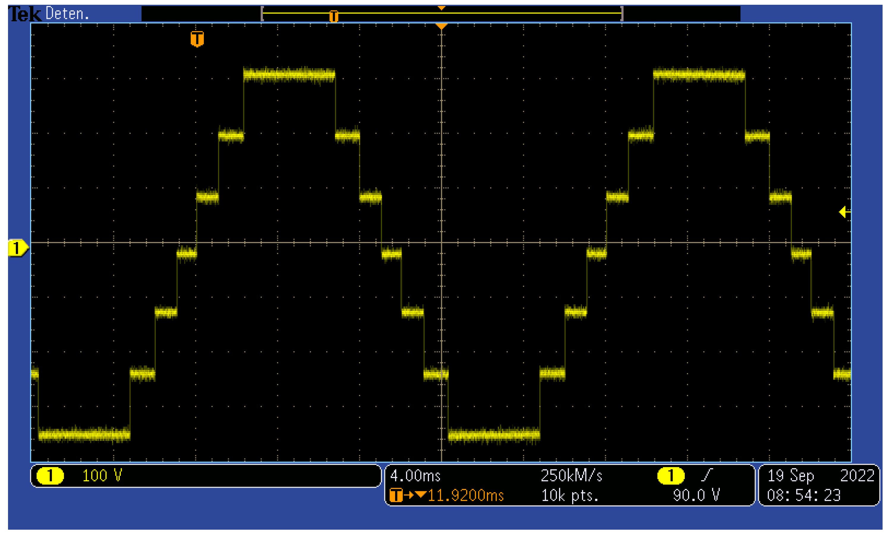
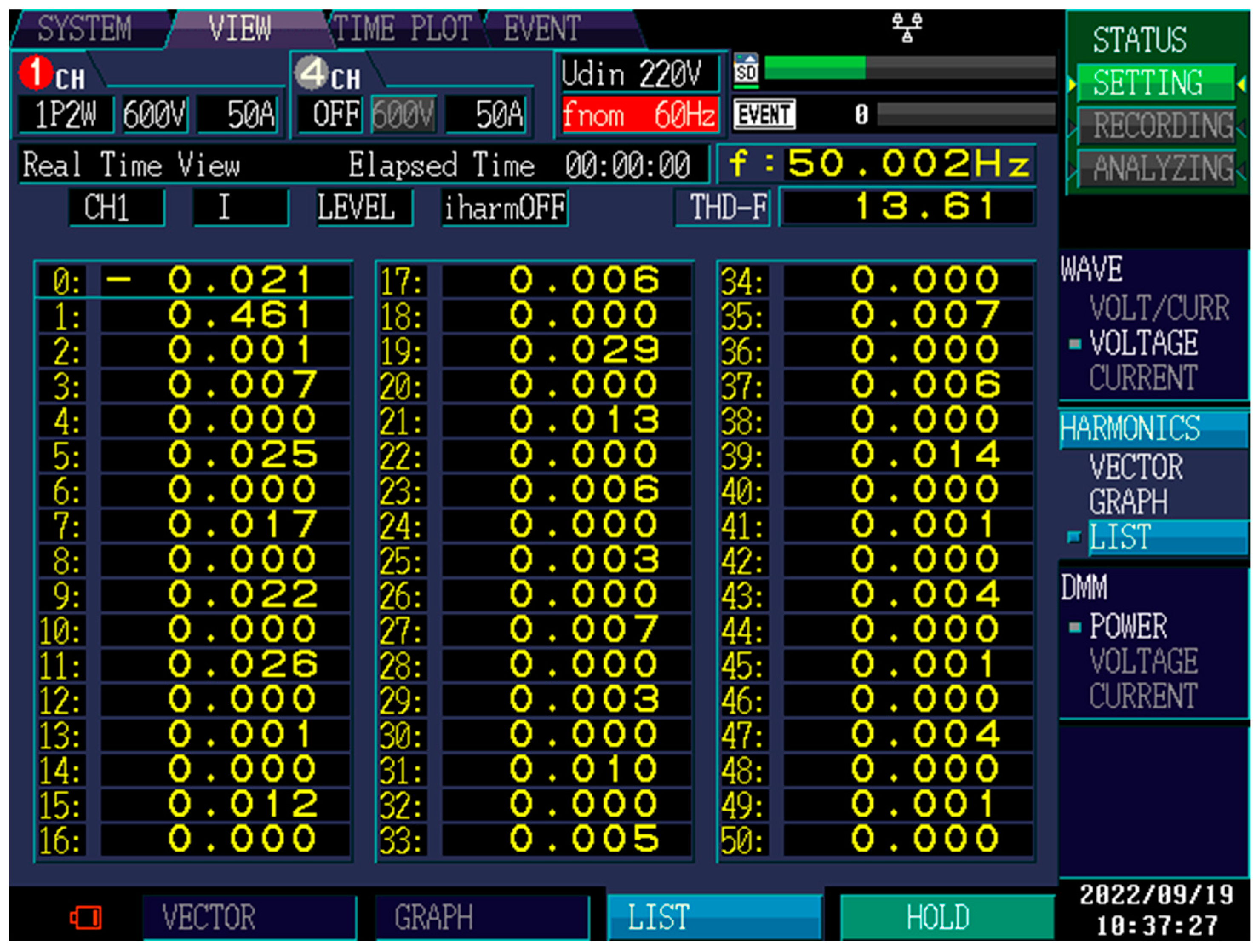
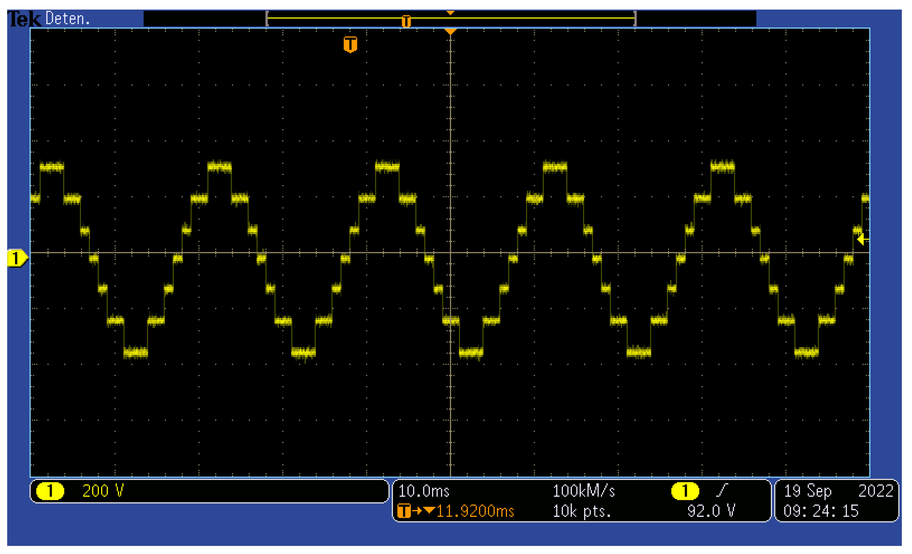
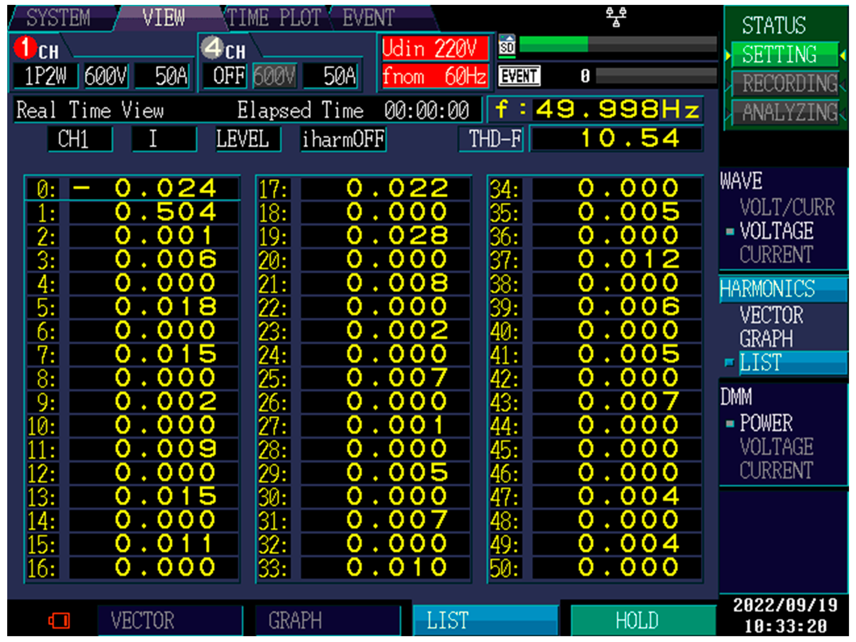
4. Experimental Results

A cascaded modular multilevel inverter was built to obtain the behavior of the proposed method and THD, resulting in a stepped output voltage of seven levels. A three-H-bridge configuration was used to generate seven output voltage levels. Figure 10 shows a CHBMLI cell, using an IRAMS10UP60A module with its respective driver circuits, implemented with a 120 V DC power supply. The switching angles obtained were implemented in the ALTERA FPGA, using look-up tables for an offline application. Figure 11 shows the experimental platform.

Figure 12 shows the implemented switching signals obtained experimentally using the set of angles in

Table 3. Best sets of angles found and their Mi.

Mi	∝1	∝2	∝3
0.97	9.80°	28.63°	64.2°
1.05	8.69°	27.89°	49.81°

. It is observed in the figure that the lines are composed of 3 colors; the blue color indicates that it is off, the green color indicates that it is on, and the yellow color indicates a signal being in transition.

Figure 13 shows the output voltage waveform obtained experimentally using the angles in Table 3 with a modulation index of 0.97.

Figure 14 shows the table of harmonic values from the fundamental to the 50th harmonic. It is observed that the THD value is 13.61%.

Figure 15 shows the output voltage waveform experimentally using the angles in Table 3 with a modulation index of 1.05.

Figure 16 shows the table of harmonic values from the fundamental to the 50th harmonic. It is observed that the THD value is 10.54%.

5. Discussion

In recent years, metaheuristic methods have been implemented to reduce THD in multilevel inverters. Among these methods, the DE algorithm has stood out for its easy implementation and fast convergence; the DE algorithm has excelled in several research areas.

The following table was created with the data obtained from the simulation (performed in Matlab Simulink) and the experimental tests.

Table 4. THD value (%) comparison between simulation and experimental tests.

Mi	Simulation	Experimental
0.97	12.98	13.61
1.05	10.46	10.54

shows the percentage of THD obtained. For the Mi of 0.97, the THD obtained in the simulation was 12.98%, while the THD obtained from the tests was 13.61%. A 0.63% difference between the simulation and experimental percentages.

For the Mi of 1.05, the THD obtained in the simulation was 10.46%, and the THD in the tests was 10.54%—a difference of 0.08%. The difference in both THD is negligible.

In both simulation and testing, there is a difference of approximately 3% of THD from the obtained Mi.

6. Conclusions

The differential evolution algorithm; is recognized as an efficient and robust optimizer. Usually, differential evolution outperforms its counterparts in efficiency and robustness.

In this paper, the differential evolution algorithm has been analyzed and implemented in a seven-level cascaded single-phase multilevel inverter (CHBMLI) to obtain the sets of possible switching angles by varying the modular index (Mi).

The simulation of the differential evolution algorithm implemented in the seven-level CHBMLI was performed in MATLAB/Simulink software.

The set of angles obtained (without considering the Mi) reduced the THD percentage to 10.46 (Mi of 1.05).

Remembering that the Mi must be less than one, it was found that the Mi that satisfies the established limits and has a decent THD reduction was 0.97, with 12.98% THD.

With these two sets of angles, tests were performed on a seven-level CHBMLI. THDs of 10.54% (Mi = 1.05) and 13.61% (Mi = 0.97) were obtained.

In both simulation and testing, there was a difference of approximately 3% in THD from the obtained Mi. The differential evolution algorithm aims to find the optimal angle sets to reduce THD and provide a suitable modular index for the output load.

In conclusion, effectively minimizing the THD value in an MLI can affect the inverter output voltage, making the Mi inadequate.

Consideration should be given to whether a high modulus value is required, but not to a low THD or a low THD with poor modulus value for that load.

References

1. Kumar, D.; Gandhi, B.G.R.; Bhattacharjya, R.K. Firefly Algorithm and Its Applications in Engineering Optimization. In Nature-Inspired Methods for Metaheuristics Optimization, Algorithms and Applications in Science and Engineering; Bennis, F., Bhattacharjya, R.K., Eds.; Springer: Berlin/Heidelberg, Germany, 2020; Volume 16, p. 503. [Google Scholar]
2. Qing, A.; Lee, C.K. Differential Evolution in Electromagnetics; Springer: Berlin/Heidelberg, Germany, 2010; Volume 4. [Google Scholar]
3. Qing, A. Differential Evolution Fundamentals and Applications in Electrical Engineering; John Wiley & Sons (Asia) Pte Ltd.: Hoboken, NJ, USA, 2009; ISBN 9780470823941. [Google Scholar]
4. Kabalci, E. Multilevel Inverters Introduction and Emergent Topologies. In Multilevel Inverters; Kabalci, E., Ed.; Academic Press: Cambridge, MA, USA, 2021; pp. 1–27. ISBN 9780128216682. [Google Scholar]
5. Upadhyay, D.; Khan, S.A.; Ali, M.; Tariq, M.; Sarwar, A.; Chakrabortty, R.K.; Ryan, M.J. Experimental Validation of Metaheuristic and Conventional Modulation, and Hysteresis Control of the Dual Boost Nine-Level Inverter. Electronics 2021, 10, 207. [Google Scholar] [CrossRef]
6. Salam, Z.; Amjad, A.M.; Majed, A. Using Differential Evolution to Solve the Harmonic Elimination Pulse Width Modulation for Five Level Cascaded Multilevel Voltage Source Inverter. In Proceedings of the 1st International Conference on Artificial Intelligence, Modelling and Simulation, Kota Kinabalu, Malaysia, 3–5 December 2013; pp. 43–48. [Google Scholar]
7. Pawar, S.V.; Morteza, S. Harmonic Elimination in Cascade Multilevel Inverter with Non Equal Dc Sources Using Genetic and Differential Evolution Algorithm. Int. J. Innov. Sci. Eng. Technol. 2015, 2, 144–150. [Google Scholar]
8. Amjad, A.M.; Salam, Z.; Saif, A.M.A. Application of differential evolution for cascaded multilevel VSI with harmonics elimination PWM switching. Int. J. Electr. Power Energy Syst. 2015, 64, 447–456. [Google Scholar] [CrossRef]
9. Chabni, F.; Taleb, R.; Helaimi, M.H. Differential Evolution based SHEPWM for SevenLevel Inverter with Non-Equal DC Sources. Int. J. Adv. Comput. Sci. Appl. 2016, 7, 304–311. [Google Scholar] [CrossRef] [Green Version]
10. Jamuna, P.; Rajan, C.C.A. A Heuristic Method: Differential Evolution for Harmonic Reduction in Multilevel Inverter System. Int. J. Comput. Electr. Eng. 2013, 5, 482–486. [Google Scholar] [CrossRef] [Green Version]
11. Sudha Letha, S.; Thakur, T.; Kumar, J. Harmonic Elimination in a Solar Powered Cascaded Multilevel Inverter Using Genetic Algorithm and Differential Evolution Optimization Techniques. In ASME International Mechanical Engineering Congress and Exposition; American Society of Mechanical Engineers: New York, NY, USA, 2015. [Google Scholar]
12. Majed, A.; Salam, Z.; Amjad, A.M. Harmonics elimination PWM based direct control for 23-level multilevel distribution STATCOM using differential evolution algorithm. Electr. Power Syst. Res. 2017, 152, 48–60. [Google Scholar] [CrossRef]
13. Storn, R.M.; Price, K.V. Differential Evolution—A Simple and Efficient Adaptive Scheme for Global Optimization Over Continuous Spaces; Technical Report TR-95–012; International Computer Science Institute: Berkeley, CA, USA, 1995. [Google Scholar]
14. Gutiérrez, D.; López, J.M.; Villa, W.M. Metaheuristic Techniques Applied to the Optimal Reactive Power Dispatch: A Review. IEEE Lat. Am. Trans. 2016, 14, 11. [Google Scholar] [CrossRef]
15. Zhang, J.; Sanderson, A.C. Adaptive Differential Evolution: A Robust Approach to Multimodal Problem Optimization (Adaptation, Learning, and Optimization, 1); Springer: Berlin/Heidelberg, Germany, 2009; Volume 1. [Google Scholar]
16. Medina, I.R. Algoritmos Bioinspirados: Una Revisión Según sus Fundamentos Biológicos; University of Manchester: Hong Kong, China, 2014. [Google Scholar]
17. Bałchanowski, M.; Boryczka, U. Aggregation of Rankings Using Metaheuristics in Recommendation Systems. Electronics 2022, 11, 369. [Google Scholar] [CrossRef]
18. Bilal; Pant, M.; Zaheer, H.; Garcia-Hernandez, L.; Abraham, A. Differential Evolution: A review of more than two decades of research. Eng. Appl. Artif. Intell. 2020, 90, 103479. [Google Scholar] [CrossRef]
19. Price, K.; Storn, R.; Lampinen, J. Differential Evolution A Practical Approach to Global Optimization; Springer: Alemania, Germany, 2005; p. 542. ISBN 978-3-540-31306-9. [Google Scholar]
20. Malik, H.; Iqbal, A.; Joshi, P.; Agrawal, S.; Bakhsh, F.I. Metaheuristic and Evolutionary Computation: Algorithms and Applications; Springer Nature: Singapore, 2021; p. 830. ISBN 978-981-15-7571-6. [Google Scholar]
21. Montes, E.M. Paradigmas emergentes en algoritmos bio-inspirados. In Inteligencia Aritificial; Alfaomega, Ed.; Alfaomega: Mexico City, Mexico, 2006; pp. 504–533. [Google Scholar]
22. Ronkkonen, J.; Kukkonen, S.; Price, K.V. Real-Parameter Optimization with Differential Evolution. In Proceedings of the IEEE Congress on Evolutionary Computation, Edinburgh, UK, 2–5 September 2005; p. 8. [Google Scholar]
23. Castillo, E.J. Esquema Adaptativo para el Manejo de Restricciones de Límite en Problemas de Optimización Numérica Restringida. Ph.D. Thesis, Centro de Investigación en Inteligencia Artificial Universidad Veracruzana Xalapa, Veracruz, Mexico, 2019. [Google Scholar]
24. Juárez-Castillo, E.; Pérez-Castro, N.; Mezura-Montes, E. An Improved Centroid-Based Boundary Constraint-Handling Method in Differential Evolution for Constrained Optimization. Int. J. Pattern Recognit. Artif. Intell. 2017, 31, 1759023. [Google Scholar] [CrossRef]
25. Yong, J. Optimization Theory a Concise Introduction; World Scientific Publishing Co. Pte. Ltd.: Singapore, 2018; ISBN 9813237643. [Google Scholar]
26. Chong, E.K.P.; Zak, S.H. An Introduction To Optimization, 4th ed.; John Wiley & Sons, Inc. Publication: Hoboken, NJ, USA, 2013; ISBN 978-1-118-27901-4. [Google Scholar]
27. Sánchez Vargas, O.; De León Aldaco, S.E.; Aguayo Alquicira, J.; López Núñez, A.R. Evolutionary Metaheuristic Methods Applied to Minimize the THD in Inverters: A Systematic Review. Eur. J. Electr. Eng. 2021, 23, 237–245. [Google Scholar] [CrossRef]
28. Hamzah, H.H.; Ponniran, A.; Kasiran, A.N.; Harimon, M.A.; Gendum, D.A.; Yatim, M.H. A Single Phase 7-Level Cascade Inverter Topology with Reduced Number of Switches on Resistive Load by Using PWM. J. Phys. Conf. Ser. 2018, 995, 012061. [Google Scholar] [CrossRef]
29. Siddiqui, N.I.; Alam, A.; Quayyoom, L.; Sarwar, A.; Tariq, M.; Vahedi, H.; Ahmad, S.; Mohamed, A.S.N. Artificial Jellyfish Search Algorithm-Based Selective Harmonic Elimination in a Cascaded H-Bridge Multilevel Inverter. Electronics 2021, 10, 1402. [Google Scholar] [CrossRef]
30. Wei, S.; Wu, B.; Li, F.; Sun, X. Control Method for Cascaded H-Bridge Multilevel Inverter with Faulty Power Cells. In Proceedings of the Eighteenth Annual IEEE Applied Power Electronics Conference and Exposition., Miami Beach, FL, USA, 9–13 February 2003; pp. 261–267. [Google Scholar]
31. Sánchez Vargas, O.S.; De León Aldaco, S.E.; Aguayo Alquicira, J.; Flores Rodríguez, E.; Lozoya Ponce, R.E. Cálculo de los ángulos óptimos de conmutación para un inversor multinivel utilizando evolución diferencial. Pist. Educ. 2022, 43, 141. [Google Scholar]
Figure 1. Diagram of the stages of differential evolution.
Applsci 12 09910 g001
Figure 2. CHBMLI waveform with seven levels and three switching angles.
Applsci 12 09910 g002
Figure 3. CHBMLI inverter with RL load.
Applsci 12 09910 g003
Figure 4. The schematic diagram for CHBMLI Simulink simulation.
Applsci 12 09910 g004
Figure 5. Output peak voltage in the CHBMLI Simulink simulation.
Applsci 12 09910 g005
Figure 6. Flow chart of the methodology used.
Applsci 12 09910 g006
Figure 7. Angles vs. Mi in CHBMLI Simulink simulation.
Applsci 12 09910 g007
Figure 8. THD vs. Mi in CHBMLI simulink simulation.
Applsci 12 09910 g008
Figure 9. Harmonic spectrum generated with the MATLAB Simulink Toolbox: (a) harmonic spectrum generated with Mi 0.97; (b) harmonic spectrum generated with Mi 1.05 (minimum %THD found).
Applsci 12 09910 g009
Figure 10. Experimental H-Bridge circuit using IRAMS10UP60A module with its driver circuit.
Applsci 12 09910 g010
Figure 11. Experimental platform, multilevel topology.
Applsci 12 09910 g011
Figure 12. Experimental H-Bridge output signals.
Applsci 12 09910 g012
Figure 13. Experimental result in a 7-level CHBMLI using the switching angles found for a Mi of 0.97.
Applsci 12 09910 g013
Figure 14. Harmonic list for the experimental result in a 7-level CHBMLI with Mi = 0.97.
Applsci 12 09910 g014
Figure 15. Experimental result in a 7-level CHBMLI using the switching angles found for a Mi of 1.05.
Applsci 12 09910 g015
Figure 16. Harmonic list for the experimental result in a 7-level CHBMLI with Mi = 1.05.
Applsci 12 09910 g016