1. Introduction
The deep neural network has brought many conveniences to our daily life. However, due to adversarial examples, deploying deep neural networks in practical manufacturing or decision-making tasks is risky. Research on adversarial examples began in Computer Vision (CV), and Szegedy C et al. [
1] found that adding subtle perturbations to a normal image could cause an incorrect model output. The study on speech adversarial examples borrows ideas from the CV domain but focuses more on attacking sequential models such as the Recurrent Neural Network (RNN) [
2]. As Automatic Speech Recognition (ASR) models are deployed on systems that directly affect safety, such as smart homes and autonomous driving, research on speech adversarial examples is increasingly crucial.
Speech recognition models typically separate speech input into frames, map them to letter or word categories frame by frame, and then assemble them into sentences by decoding algorithms [
3]. Adversarial examples against ASR usually perform targeted attacks by adding subtle perturbations to normal speech so that it is transformed into the text specified by the attacker, thus covertly executing malicious commands [
4] and posing a greater security threat.
Researchers have proposed several methods for detecting speech adversarial examples. Samizade et al. [
5] developed a CNN-based speech cepstral feature classification network. Still, the method has poor generalization performance in detecting adversarial examples generated by different methods and unknown methods. Rajaratnam et al. [
6] investigated adding a large amount of random noise to a specific frequency band of the audio signal. Kwon et al. [
7] modified normal audio by adding noise, low-pass/high-pass filtering, etc. Both studies exploited the property that adversarial examples have lower robustness than normal audio. However, the effectiveness of these methods in defending against complex attacks and over long speech requires further investigation. Yang et al. [
8] segmented the speech data and calculated the consistency of the segment recognition results with the whole sequence recognition results to detect adversarial examples, but the location of the segmentation points was not universal.
The above detection methods focus on the differences between normal data and adversarial examples, but they do not incorporate the inference results of the model. There is more information in the judgment by the ASR model. For example, Park N et al. [
9] exploited the difference in the logit distribution of normal speech and adversarial examples. The method can achieve an accuracy of over 95% and detect adversarial examples generated by multiple attack methods without task flow changes or additional training.
However, it is found that this detection method is susceptible to adaptive attacks. The key insight is that Park N et al. [
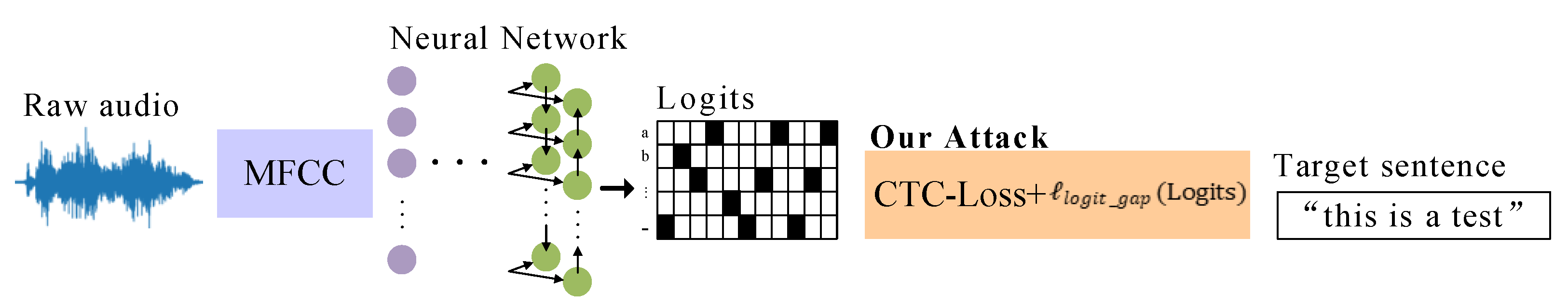
9], who exploited only one feature to detect adversarial examples. The feature uses the difference between the maximum value and the next largest value in each frame of logits to quantify the dispersion degree. To attack this feature, this paper designs a new loss function term to construct Logits-Traction attacks. The specific process is shown in
Figure 1.
The generation of speech adversarial examples is a multi-step iterative [
10] optimization procedure. In each iteration, the original loss Connectionist Temporal Classification-Loss (CTC-Loss) adds adversarial perturbation that enables the adversarial example to be transcribed in the direction of the target sentence. Meanwhile, the new loss function term
increases the intra-frame logits difference, and they are not in a completely antagonistic relationship. Thus, it is possible to make the new adversarial example closer to the original speech in the evaluation metric of intra-frame difference, thereby evading the detection mechanism of Park N et al.
However, the difference of logits between normal speech and adversarial examples has a spatial distribution. The detection method [
9] only measures this difference in one dimension. The similarity of this quantitative metric does not imply that our adversarial examples have the same logits distribution as normal speech. If alternative evaluation metrics [
11] can detect our novel adversarial examples, the adversarial example detection method based on the dispersion of logits is still valid when the attacker is unaware of the specific quantitative measure. To further investigate whether an attack method generates adversarial examples with the same logit distribution as normal speech, this paper proposes logits-based detection methods that focus on three different features, including the intra-frame mean difference, decision frame variance, and the number of delineation statistics of logits.
The main contributions of this paper are summarized as follows:
This paper analyzed three high-precision speech adversarial examples detection methods. Among them, the Logits-based detection method is the most promising because it does not need prior knowledge when detecting adversarial examples. To evade such detection, this paper also studies two representative logits in different ASR models, and further analyzes the manifestations and causes of logits distribution differences.
To quantify this difference, this paper defined logits dispersion to describe the quality of logits. A smaller dispersion of logits implies that one speech is more likely to be an adversarial example. This paper proposes a Logits-Traction attack to improve the logits dispersion. It constructs a new loss function to generate adversarial examples, and this attack is compatible with the logit types of different ASR models.
This paper extends the logit features exploited by the detection method to evaluate the effectiveness of the above attack method. It focuses on three different features, which can detect Carlini and Wagner (C&W) adversarial samples with high accuracy, proving the effectiveness of these features. These features are then used to detect the Logits-Traction adversarial examples. The experimental results show that the detection method based on these features has different degrees of accuracy decline when detecting the Logits-Traction adversarial examples, which leads to the failure of the detection method. Logit-Traction attacks can effectively avoid detection based on logits.
3. Proposed Method
To improve the similarity between adversarial examples and original speech in models with different loss functions, this paper investigates two representative logits types in ASR systems, namely sparse logits and dense logits. Then, this paper proposes the concept of logit dispersion and designs a new loss function term for the characteristics of each type of logit so that the adversarial examples are optimized in the direction of increasing logit dispersion. To explore further whether the adversarial examples generated by the innovative method can approach the logits of normal speech in several quantitative dimensions, this paper proposes three different features to calculate logits dispersion. These features are used to verify whether an adaptive attack against one metric method can simultaneously reduce the detection accuracy of three other features and show the distribution characteristics of adversarial example logits under different attack methods.
3.1. Logits Type in the ASR Model
Logits are a vector that represents the raw outputs [
27] of the neural network. In the model performing the image classification task, logits are one-dimensional sequences followed by a SoftMax layer [
28]. In the ASR task, the output of RNN is logits [
29]. It is a two-dimensional vector, which is usually transcribed into a character vector or word vector using beam search decoding and then assembled into a complete sentence.
In practice, the logits structure of the ASR model [
13,
30] can be represented as [batch_size, frames, classes], where “batch_size” represents the number of speeches in each iteration. “Frames” represents the number of frames of each speech, and is dependent on the length of the speech sequence and the MFCC window size. “Classes” represents the categories into which each frame may be transcribed.
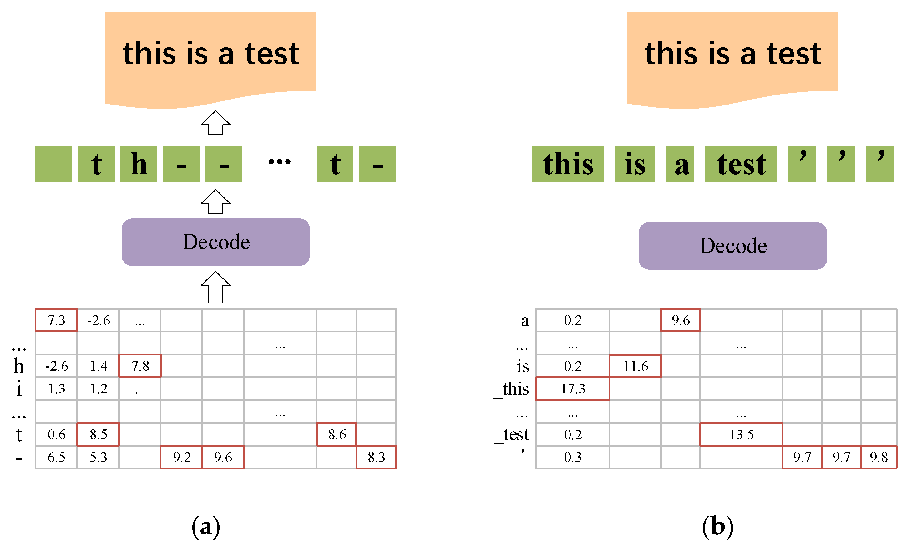
In character-level transcription (
Figure 2a), “A–Z”, “Space”, and “Blank” pseudo-characters (represented by “-”) are included in the transcription classes. “Blank” means no characters and can only be used to separate two characters. For differentiation, this paper refers to the frames with the highest value in the “Blank” category as the “blank frame” (frame 4, 5, and the last frame on
Figure 2a), and the remaining frames are called the “decision frame”. In the process of generating adversarial examples, the conversion between “blank frame” and “decision frame” is more accessible than that between “decision frame” and “decision frame”. Meanwhile, it tends to get a more significant intra-frame difference. This paper defines the logits structure of alternating “blank frame” and “decision frame” as sparse logits. ASR models using CTC loss functions, such as DeepSpeech [
13], typically includes sparse logits. During the optimization of adversarial examples, the inter-frame interactions of the sparse logit are minimal, and the faults generally are exhibited as mis-transcribed characters in words.
In word-level transcription (
Figure 2b), the transcribed classes are related to specific models, including all labelled words and word roots from the training data. The transcription of succeeding frames requires the results of the previous frames, and the output of the last state in the RNN network contains the logits information of the whole speech sequence. In this logits type, the first
“decision frames” (
on the
Figure 2b) determine the transcription result of the speech with a substantial intra-frame difference. In contrast, the subsequent
frames are meaningless “blank frames” with a near-zero intra-frame difference. This paper defines such logits with distinct bounded frames as dense logits. Dense logits are included in ASR models such as Lingvo [
30] that employ cross-entropy loss functions. Its incorrect transcription results can only originate from classes, and the mistakes are presented as successive words or root transcription errors.
Therefore, the distribution of blank frames in dense and sparse logits is significantly different. The blank frame cannot effectively affect the transcription result compared to the character frame. More weight should be given to the character frame to improve the detection accuracy. Indeed, the logit distribution of original speech and adversarial example are more different in these frames.
3.2. Logits Value of Adversarial Examples
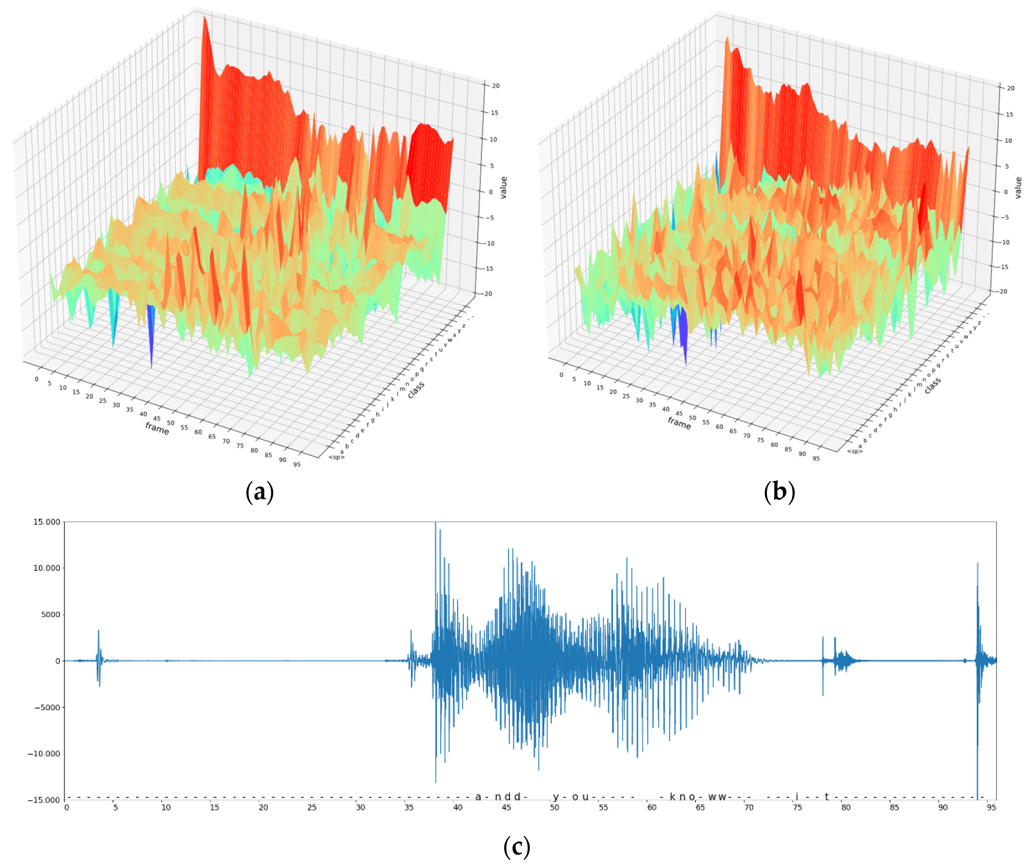
To visually show the difference in logits between the original speech and adversarial examples, this paper plots a three-dimensional representation of the logits of the original speech and adversarial examples derived from it. As shown below, the frame axis in the figure represents the MFCC frame of the speech vector. The number of coordinate points on this axis is proportional to the length of the speech audio. The class axis represents probability distribution, where the model decodes each frame into all characters, and that probability is unnormalized. The value axis represents the specific value of the above possibility. The class that has the maximum value in each frame is transcribed characters. So the transcription task can also be considered a frame-by-frame classification task. Below (a) are the logits of the original speech whose transcription result is “and you know”, and (b) are the logits of the C&W adversarial example generated based on the above original speech and whose transcription result is “This is a test”. The logits were output by the DeepSpeech model. This paper connects these points as surfaces to better show their changing process.
Figure 3a depicts the logits value of the original speech sequence, and
Figure 3c depicts the raw signal of the original speech. In it, frames 0 to 35 represent silence. The “blank” characters (denoted by “-”, the last column in 3.a class axis) score significantly higher than other classes, indicating that DeepSpeech is highly confident that these frames are transcripted to “blank”. Frames 35 to 80 are the stages of human vocalization. In these stages, each frame column has a better value on only one category, with logit values that are much lower and less changeable for other classes. In the original speech, the confidence of “blank frame” and “decision frame” is generally higher. The
Figure 3b represents the adversarial example, except for the “blank” class in the “blank frame”, which has a more significant logit value. All other logit values are minor. In the “decision frame”, each frame column has multiple large values, and DeepSpeech only recognizes them as the target transcription with weak confidence.
To quantify this difference numerically, Park N et al. proposed a detection method based on the “distribution of the difference between the maximum value of logit and the second largest value” by adding Gaussian noise to the logits. Their method assumes that frames with a minor difference are more susceptible to maximum bit reversal when the noise follows the same distribution, leading to altered transcription results. As shown in
Figure 3, the speech with more altered transcriptional effects after adding noise is more likely to be an adversarial example. After calculating the number of erroneous characters caused by adding noise to the logit, the error threshold can be determined at a statistical level, and speech adversarial example detection independent of the network structure is implemented.
This paper defines the degree of disparity between the values of the classes in the “decision frame” of logits as the logit dispersion. In dense logits, it is sufficient to calculate by the values of “decision frames” that have the potential to affect the final transcription result. However, in sparse logits, the values of the “blank” pseudo-characters class in all “decision frames” must be removed.
3.3. Logits-Traction Adversarial Example Generation
3.3.1. Inspiration
In computer vision, the C&W L2 attack [
31] for the image classification task sets the confidence in the one-dimensional logit sequence to calculate the intra-frame difference feature. The loss term to perform the targeted attack is:
where
represents the adversarial example,
represents the logit value of the
class,
is the target class, and
is the confidence of the adversarial example. To achieve target attacks, a larger
is more likely to cause model misclassification.
Such a loss function is a piecewise function, and it works well in classification tasks. The same mechanism in speech adversarial examples will be affected by logits frame [
32,
33], and it is impractical to set a
value for each frame. This paper only comprehensively considers the intra-frame logits difference of all frames, and generates adversarial examples with an overall higher logit intra-frame difference based on the fact that adversarial examples are always optimized to decrease the loss function value.
3.3.2. Threat Model
For a given speech signal sequence and target transcribed phrase , this paper constructs another audio waveform so that , and the logits dispersion of the generated adversarial examples is close to normal speech. To generate adversarial examples, the network structure and parameters of the target model are completely evaluated, and then they are optimized and tested in the digital realm. This is a typical tactic for white-box attacks.
3.3.3. Logits-Traction Loss Function
In both image and audio, generating adversarial examples against a white-box model can be considered as updating
via gradient descent [
34,
35] on a predefined loss function:
where
denotes the loss function of the target model and
denotes the distortion measure function. Parameter
weighs the relative importance of achieving adversarial attacks and reducing adversarial perturbations.
Due to the interframe interaction and the additional decoding steps in ASR, it is not easy to construct a loss that corresponds to the optimization objective.
Since the improvement of the loss does not need to consider the interaction between frames and additional decoding steps, the literature designs a loss function term, that improves the attack efficiency and the robustness of adversarial examples. Our method draws on this and aims to construct adversarial examples with new features. In our method, the optimization objective is extended as follows:
In the process of backpropagation, this loss function generates that achieves target transcription while producing a minimal . The formal description of will be elaborated below.
Our optimization objective is composed of the following three components:
denotes the original loss function used in the ASR model. The loss of sparse logits is CTC-Loss, and the loss of dense logits is cross-entropy loss function. Using the same loss function as the original model to generate adversarial examples is based on the following observation:
measures the logits value gap of the original output, calculates the difference between the maximum value and the second-highest value in all categories for each frame, and then adds these values together. The specific calculation method is shown in Algorithm 1.
| Algorithm 1: Measurement Method |
Input:, the original output of the adversarial example passing through the ASR model during each iteration.
Output: , a vector describing the intra-frame difference of logits. |
initialize for initialize for set return
|
where
denotes batch_size,
denotes frames, and
denotes classes; “0:
b” means traversing over values from
to
, and “:” means it traverses all the values of the dimension in symbol resides (
ie. to
). A smaller
means that the neural network has higher confidence in the current transcription result.
measures adversarial perturbations, and it is defined as:
This paper adds the term to filter the C&W adversarial examples further. This may make the adversarial perturbations satisfy both constraints, resulting in speech distortion. Therefore, is added to limit the disturbance by penalizing adversarial perturbations with large absolute values.
3.4. Detection Based on Logits Dispersion by Other Three Features
This section further explores the effectiveness of our attack method. Given that the logit distribution of adversarial examples differs from that of normal speech, this paper designs detection mechanisms that focus on different features. The statistical features of logits in several other dimensions are calculated, such as intra-frame mean difference, decision frame variance, and the number of delineation statistics. It is checked whether Logits-Traction adversarial examples affect the detection accuracy based on these features.
As described in
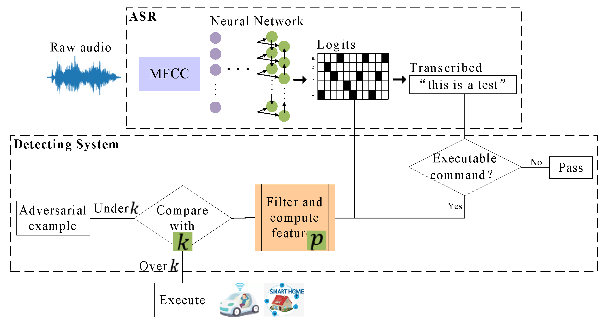
Section 3.2, the number of “decision frames” in dense logits is small, and each frame has too many possible categories. Adding noise to the logits by Park N et al. cannot distinguish between normal speech and adversarial examples. Another drawback of this method is that the random noise mechanism may produce inconsistent findings for numerous detections of the same speech. To this end, this paper designs new detection methods, and the detection system deployment [
36] is shown in
Figure 4:
This detection system consists of three fixed logits feature calculation algorithms, a hyperparameter and a threshold . and are only related to the protected model. When a text transcribed by ASR is recognized as an executable command, the detection system performs feature calculation on its logits. At first, the algorithm screens out logit values that satisfy the condition, then applies the feature calculation algorithm to acquire the evaluation value and compares this value with the threshold k. Those exceeding the range of are considered adversarial examples.
3.4.1. Detection Based on the Intra-Frame Mean Difference
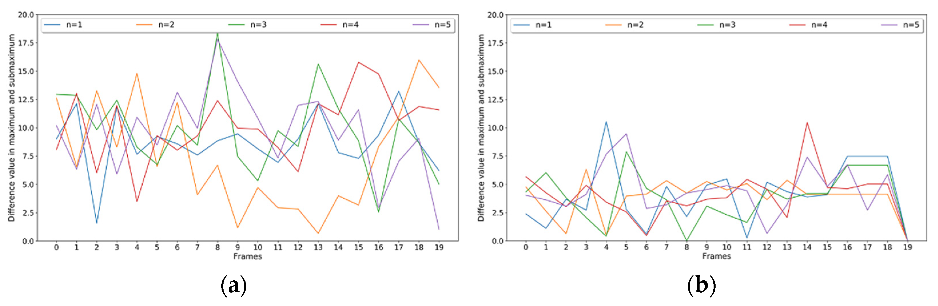
Figure 3 illustrates that the difference between the maximum value and the next largest value in logits differs for normal speech and adversarial examples. The dense logits also show the identical pattern as shown in
Figure 5:
These five adversarial examples are generated from the code [
37] provided in the literature [
15]. It indicates that adversarial examples have a smaller intra-frame difference than normal speech. This paper quantifies this difference by calculating the sum between the maximum value and the next largest value for all decision frames. The phenomenon that long text speech with a significant difference sum is more likely to be judged as normal speech can be avoided by dividing by the number of decision frames:
where
denotes the set of serial numbers of character frames and
denotes the maximum value of the
frame. The obtained
is compared with the threshold
, and those less than
are judged as adversarial examples.
3.4.2. Detection Based on the Variance of Filtered Values
The optimization objective of adversarial examples is to introduce an adversarial perturbation to yield the target expression. However, it does not suppress its original expression. The original expression may shift and spread in the adversarial perturbation. That will result in adversarial examples with slight logit variance. Focusing on this issue, this paper designs a statistical detection method based on the variance of filtered values so that under the same calculation method, the logit variance of adversarial examples can be smaller, and the logit variance of normal speech can be larger. The filter mechanism can distinguish adversarial examples from normal speech more clearly.
In the sparse logit ASR model, values greater than the hyperparameter
p in the speech logits to be detected must be screened, and the variance of the non-negative values in matrix
is derived as the logit evaluation index:
where
,
denotes the average of all values greater than
in this non-sparse matrix
where
,
denotes the number of all values greater than
in matrix
.
In the dense logit ASR model, the variance of non-negative values in matrix is calculated as the logit evaluation index, and the calculation method is the same as the above formula. Finally, is compared with the statistical threshold , and those less than the threshold are judged as adversarial examples.
3.4.3. Detection Based on the Number of Delineation Statistics
This method is still based on the assumptions introduced in
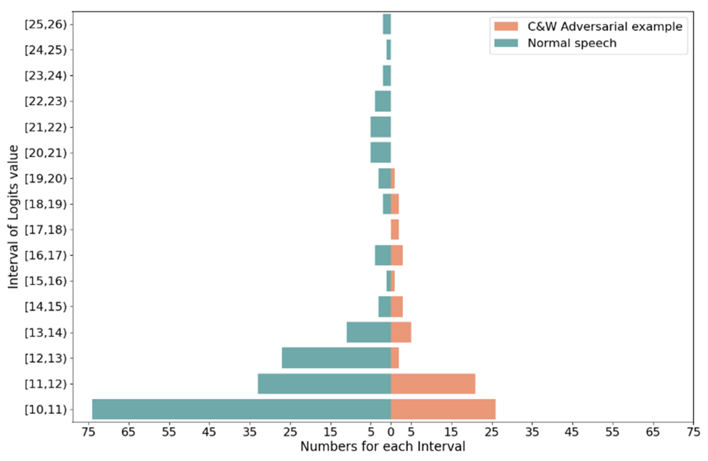
Section 3.4.2 but is not concerned with the fluctuation of values. The following
Figure 6 shows the distribution interval statistics of logits values of a speech and its adversarial examples in the Lingvo model. The original transcription of the speech is “THE MORE SHE IS ENGAGED IN HER PROPER DUTIES THE LESS LEISURE WILL SHE HAVE FOR IT EVEN AS AN ACCOMPLISHMENT AND A RECREATION”, and the target sentence to generate the antagonistic example is “OLD WILL IS A FINE FELLOW BUT POOR AND HELPLESS SINCE MISSUS ROGERS HAD HER ACCIDENT”.
It has a similar pattern to
Figure 3. That is, the magnitude of logits value of adversarial examples is generally less than that of normal speech. This method just counts the number of values in the decision frames that are bigger than the filtered value
:
.
The speech is judged as an adversarial example if is less than a threshold value. However, this method is easily affected by the number of decision frames and can only be used in adversarial example detection with similar text lengths.
4. Experimental Evaluation
To verify the effectiveness of our attack, the code [
38] in the paper [
9] is reproduced, the Logits-Traction (LT) adversarial examples are tested, and their detection accuracy is compared with that of C&W adversarial examples. Then, to evaluate the efficacy of our proposed detection features, C&W adversarial examples are built on multiple models and datasets. They are combined with the original speech data to create a new dataset and be tested. Finally, the accuracy of the above detection in detecting novel adversarial examples is tested to demonstrate that Logits-Traction adversarial examples can evade the logits-based detection features.
4.1. Dataset and Experiment Setup
Target ASR model: The target model of this paper for the experiments covers two types of logits. For sparse logits, the DeepSpeech model with the CTC loss function is selected, and for dense logits, the Lingvo model with the cross-entropy loss function is selected.
Source dataset: (1) LibriSpeech (Libri) [
39]. The LibriSpeech dataset is from the LibriVox project. It is composed of English speech data with a sampling rate of 16 kHz, and the recording environment is relatively stable. This paper randomly selects speech data on the “test-clean” branch. (2) Mozilla Common Voices (MCV) [
40]. The MCV dataset is a public speech dataset contributed by volunteers worldwide. The recording environment is inconsistent, and the volume levels vary. To be consistent with LibriSpeech, this paper uses the “sox” tool to downsample each speech from 48 kHz to 16 kHz, and randomly select speech data from it.
Dataset in our experiment: This paper randomly selects 600 speeches from each dataset as the original speech. The number of transcribed words ranges from 3 to 10, so the speech durations are approximately the same as those in the original papers [
9]. However, only five target phrases are set in that study, leading to monotonous logits distribution of the adversarial example, thus making the success rate of our attack unrealistically high. To truly reflect the strength of our attack against the detection method, this paper randomly selects 100 transcriptions from 600 speeches as target phrases. Then, using the remaining 500 speeches as original speeches, the C&W adversarial example dataset and logits-Traction adversarial example dataset were created on DeepSpeech and Lingvo models, respectively. The success rate of detection based on three features is evaluated by C&W adversarial example dataset. The decline in detection success rate is evaluated on the LT adversarial example dataset.
This paper adopts accuracy, false-positive rate (FPR), and false-negative rate (FNR) as evaluation indicators. The accuracy rate is used to evaluate the quality of the detection method; FPR represents the proportion of the original speech detected as an adversarial example; FNR represents the proportion of adversarial examples detected as the original speech. FPR and FNR are negatively correlated due to the usage of threshold division for judgment.
4.2. Logits Traction Attack Effectiveness Evaluation
Since the original detection method can only detect sparse logits, his paper tests the Logits-Traction attack on the DeepSpeech v0.4.0 system. When constructing the adversarial example dataset, the Adam [
41] optimizer is used. The learning rate is set to 100, and the maximum number of iterations is set to 1000. This paper performs detection on the two established adversarial datasets with the same configuration. The experimental results are as follows:
It can be seen from
Table 1 that the FNR is 37.6% when detecting C&W adversarial examples, indicating that the detection method [
9] has a limited detection success rate when the target phrases of the adversarial examples are abundant. In this more realistic configuration, LT attacks reduce the success rate of the LOGITS NOSIE detection method, proving that our LT adversarial examples are difficult to detect, thus evading the logits-based detection.
Meanwhile, an excessive FPR for raw speech on the MCV dataset can be observed. After auditioning and analyzing the misclassified original speech, it is found that they are generally of poor quality or low volume and being chaotically transcribed by DeepSpeech. Since the detection system is deployed in the location shown in
Figure 5, where logits are detected after transcription and before command execution, the high FPR of the original voice will not affect the regular operation of the detection system.
4.3. Logits Dispersion Detection Effectiveness Evaluation
When the detection algorithm is deployed, the defender only has information about the model to be protected, and it does not know the data source of the original speech used by the attacker. Therefore, the hyperparameter and threshold set by each detection algorithm should be fixed, and only change with the protected model. The current test parameters are set as follows:
Logit- detection. It does not require a hyperparameter . If the average difference between the largest and second largest values exceeds the threshold , it is determined that the logits belong to the original speech;
Logit- detection. In DeepSpeech, is set to , which means to calculate the variance of the numbers whose logit value is greater than in all decision frames. If the variance is greater than the threshold , it is determined that the logits belong to the original speech. Similarly, is set to in Lingvo;
Logit- detection. In DeepSpeech, is set to 9, which means to count the number of values greater than 9 in all decision frames. If the number is greater than the threshold , it is determined that the logits belong to the original speech. Similarly, is set to in Lingvo.
The detection results of the three detection methods on the C&W adversarial examples are presented in
Table 2:
It can be seen from
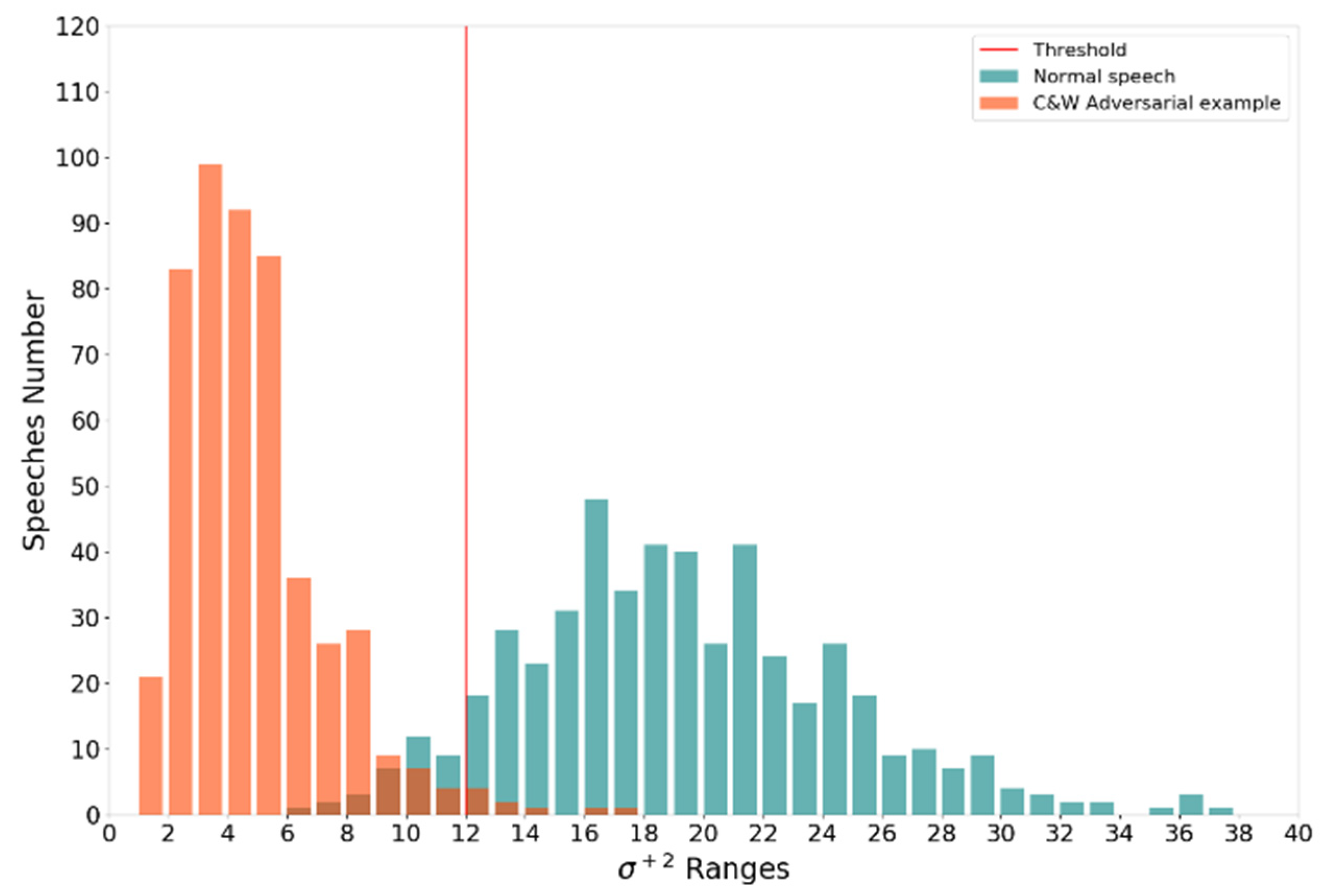
Table 2 that all three features have high accuracy on the LibriSpeech dataset, and the three features in the DeepSpeech and Lingvo models have similar detection accuracy distributions, indicating that our three detection methods based on logit dispersion are efficient. We take the detection using
features on the Lingvo system as an example, which achieved the highest detection accuracy on the LibriSpeech dataset. Their detection results are shown in
Figure 7:
The of C&W adversarial examples less than 12 can be correctly detected. A few normal speech values less than 12 are mistakenly judged as adversarial examples. There is a clear dividing line between this two. The threshold , is the dividing line between the adversarial example and normal speech.
Second, this paper uses the MCV dataset as comparison experiments, and its FNR is lower, meaning that our detection features can effectively detect even adversarial examples generated based on chaotic speech. Finally, the detection accuracy between our three features is similar. This is because the feature of difference, variance, and the absolute number of values are not entirely independent in the calculation. These features are all affected by the more significant value in logit decision frames.
Meanwhile, several experiments show that the detection accuracy cannot be improved effectively by tuning the hyperparameter and the threshold . That is an inherent drawback of these three features in quantifying logit dispersion. They cannot draw a clear demarcation line between the original data and the adversarial examples, and false and missed detections always exist.
4.4. Effectiveness of Logits Traction Attack against Our Three Detections
In this experiment, the values of the parameter
and threshold
obtained from each feature in the above experiments are preserved. These features are used to detect LT adversarial examples. This section only focuses on the FNR decline caused by LT adversarial examples, which means that the proportion of adversarial examples is not detected by the above features,
Table 3:
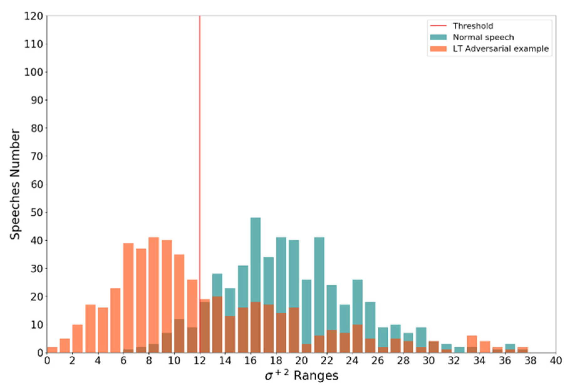
The experimental results show that the Logits-Traction adversarial examples can evade the logit dispersion-based detection. A false negative rate of more than 50% at the statistical level makes these three features no longer practical. The quantified logits dispersion of Logits-Traction adversarial examples has a more similar distribution to that of the original speech. As shown in
Figure 8, there is no reasonable threshold to distinguish adversarial examples from the original speech.
Meanwhile, compared with DeepSpeech, the effect of the Logit-Traction attack on the Logit- feature in Lingvo is not obvious. This result indicates that the feature of LT adversarial is still inferior to that of the original speech. Due to the expression in the original speech, the logits value of the adversarial example has difficulty in reaching the same level. That is the native advantage of the Lingvo system. Customizing the adversarial example detection system for Lingvo can affect the number of larger values in logits.
The experiments in
Section 4.3 and
Section 4.4 mean that our Logit-traction attack will bring the logit distribution of the antagonistic example closer to the ideal Logit distribution of normal speech. However, the attack success rate is also affected by the characteristics of interest in the detection method.


