Wiener Filter and Deep Neural Networks: A Well-Balanced Pair for Speech Enhancement

Abstract

This paper proposes a Deep Learning (DL) based Wiener filter estimator for speech enhancement in the framework of the classical spectral-domain speech estimator algorithm. According to the characteristics of the intermediate steps of the speech enhancement algorithm, i.e., the SNR estimation and the gain function, there is determined the best usage of the network at learning a robust instance of the Wiener filter estimator. Experiments show that the use of data-driven learning of the SNR estimator provides robustness to the statistical-based speech estimator algorithm and achieves performance on the state-of-the-art. Several objective quality metrics show the performance of the speech enhancement and beyond them, there are examples of noisy vs. enhanced speech available for listening to demonstrate in practice the skills of the method in simulated and real audio.

1. Introduction

The development of communication devices has increased the number of available channels for audio acquisition. However, some applications may not take advantage of this fact. For instance, the audio from telephone communications is in a mono-channel format. So, the post-processing of the telephone speech has to deal with the challenging task of single-channel speech enhancement.

Speech enhancement (SE) algorithms attenuate the noise pattern in the observed speech signal—the noisy speech—to increase the speech perceived quality. An established approach for single-channel SE is the family of spectral-domain speech estimator algorithms, which are based on the gain-based approach [1,2]. In this framework, the noisy speech is transformed into the time–frequency (t-f) domain. Then an estimated gain is applied to the t-f speech representation in order to obtain an enhanced version. Finally, a synthesis stage applies an inverse transformation to the enhanced t-f speech to obtain the signal back into the time domain. The best-known methods among this framework are the Wiener filter [3], spectral subtraction (SS) [4], short-time spectral amplitude (STSA) [5], and the log-spectral amplitude estimator (LSA) [6]. In general, these approaches rely on estimations of the a priorisignal-to-noise ratio (SNR), which are used to compute the gain function to determine the attenuation of noise-dominated t-f regions. Although many SE algorithms follow the gain-based approach, they mainly differ in the way the a priori SNR is estimated and in which gain function they use. The design of the gain function and the accuracy of the a priori SNR estimation can become the main weakness of the SE method. In realistic scenarios, the dynamic fast changes of non-stationary impulsive noise and the mixture of noise types, including speech-correlated noises, propose significant challenges for statistical SNR estimators [7].

The high capability of deep learning approaches for finding underlying relations in the data and providing substantial representations from them has attracted the attention of SE algorithms. There is a previous work studying different deep neural networks (DNN) based estimations of the SNR and the gain function. The work of Xia et al. [8,9] firstly approach the DNN-based SE by supporting the Wiener filtering with a weighted denoising autoencoder. This estimates the clean speech by subband and then uses it for estimating the short-term a priori SNR and the filter gain function. Similarly, from the mono-aural speech separation, the t-f masking approach with ideal binary/ratio masking (IBM/IRM) [10] is used for performing feature enhancement in automatic speech recognition (ASR) [3,11]. In [12,13], the authors proposed a supervised learning algorithm for IRM estimation to perform noise-robust ASR. Then, Refs. [14,15,16,17] extensively used the DL-based estimation of IBM and IRM for hearing-aids purposes also applied to ASR. For cochlear implant applications, Refs. [18,19,20] extended the SE using DNN based on IRM to novel speakers and proposed an approach suitable for practical applications with low latency. Recently, DeepMMSE [21] attempted to estimate the power spectral density (PSD) of non-stationary noise using deep learning and they obtained very promising results. Related to this work, in [22], the authors estimated the a priori SNR with a residual long short-term memory (ResLSTM) network, achieving improvement in the performance of traditional minimum mean square error (MMSE) estimators. More recently, the same authors extended the study by including more architectures, such as residual networks and multi-head attention [23] and also using multiple objective quality and intelligibility measures to achieve improved enhancements of the noisy speech.

This paper proposes a deep learning (DL) based approach to estimate the Wiener filter function and perform SE supported on the classical LSA speech estimator. We tested the performance by using directly the LSA speech estimator and also its optimally modified version (OMLSA) [24], which considers the speech presence probability (SPP). During the study, we explored the key points of the SE algorithm and accordingly the best use of deep learning. In [21,22,23], the deep learning approach targets the estimation of the a priori SNR, which is complemented with a compression function for making possible the training of the network. Then, the authors employed the a priori SNR estimation for computing the Wiener filter and proceed with the SE traditional algorithm. By analyzing this strategy, we realized that the high dynamic range of the SNR $(-\infty ,\infty )$ is a hard objective to accurately be estimated by a deep structured network. This is the reason why a compression function was employed in [23] to avoid convergence problems during the training. Furthermore, SNR is an intermediate step to finally obtaining the Wiener filter function to feed the SE algorithm. So, it is more practical that the network was able to provide a more robust estimation of directly learning the Wiener filter.

The main contribution of this paper relies on the use of the deep learning approach for directly estimating the Wiener filter instead of the a priori/posteriori SNR, which could bring accuracy and convergence troubles at the training step. Further contributions of this paper are as follows:

• A data-driven Wiener filter estimator that can be generalized to different approaches of the classical spectral-domain speech estimator algorithm, tested with LSA and OMLSA speech estimators.
• In the line of previous works, this paper demonstrates the usefulness of deep learning for expanding the application scope of established speech enhancement schemes in realistic scenarios with challenging environmental noisy patterns.

Examples of enhanced signals are available (http://dayanaribas.vivolab.es/DEMOenhancement/index.html (accessed on 1 September 2022)).

In the following, Section 2 introduces the speech enhancement task through the spectral-domain speech estimator algorithm. Then, Section 3 describes the proposal followed by the deep structured network architecture in Section 4. The experimental setup is in Section 5. Finally, Section 6 presents the results and discussion, and Section 7 concludes the paper.

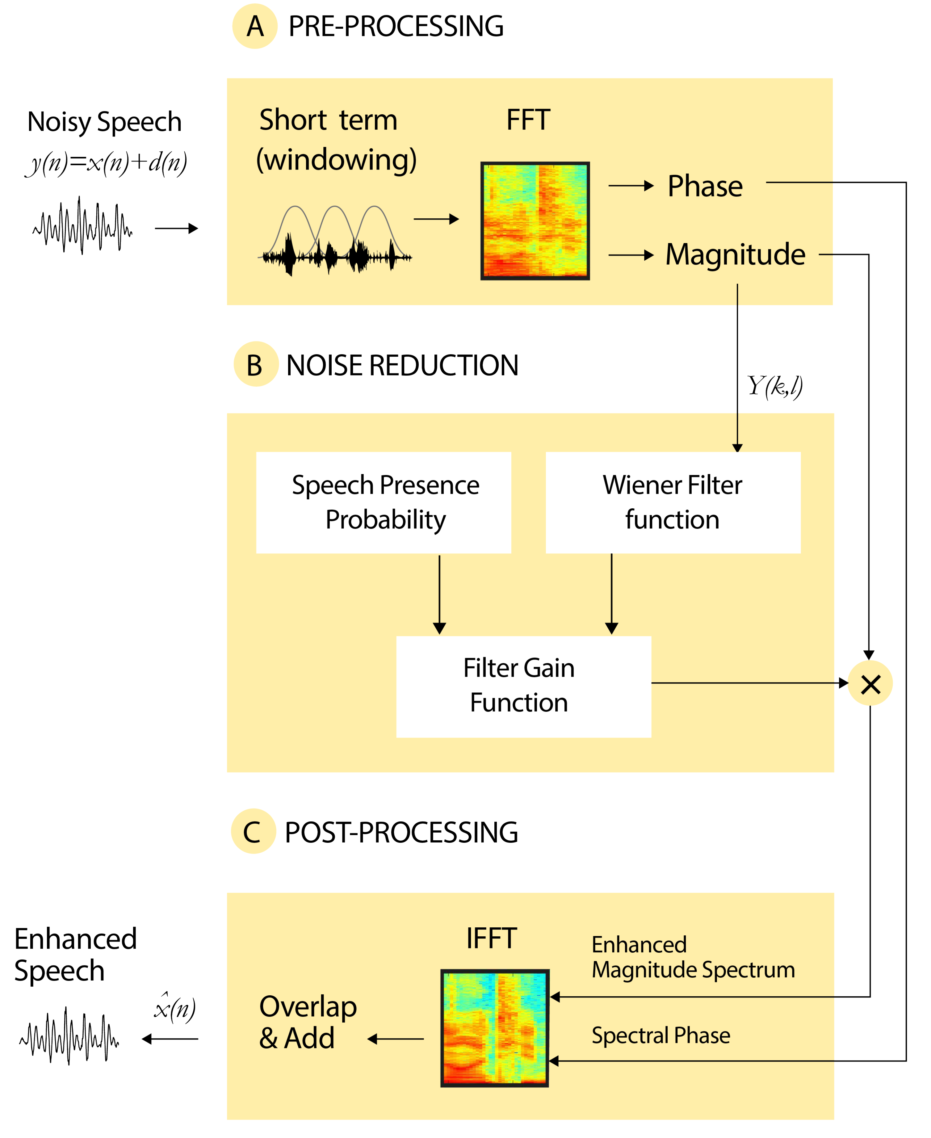
2. Speech Enhancement

Let $y\left(n\right)$ denote the observed noisy speech signal given by $y\left(n\right)=x\left(n\right)+d\left(n\right)$ with $x\left(n\right)$ the clean speech, $d\left(n\right)$ the additive noise, and n the discrete-time index. The pre-processing stage for performing speech enhancement in the spectral domain starts with a short-term speech analysis of the segmented $y\left(n\right)$ into overlapping frames through the application of a window function. Then, a short-term Fourier transform (STFT) is used to obtain the spectral representation:

$$Y(k,l)=\sum _{n=0}^{N-1}y(n+lM)h\left(n\right)e^{-j(2\pi /N)nk},$$

(1)

where l is the time frame index, k is the frequency bin index, $h\left(n\right)$ is the analysis window of size N, and M is the number of samples between two frames.

Figure 1 depicts the spectral-domain speech estimator algorithm. The power spectrum ${\left|Y(k,l)\right|}^2$ is used as input of the noise reduction block, while the spectral phase is kept apart for the last block of post-processing for speech reconstruction. The output of the system, $\widehat{x}\left(n\right)$, is an enhanced version of the noisy signal as similar as possible to clean speech.

The core of the enhancement method is depicted in the central block. This approach is the paradigm followed by the family of spectral-domain speech estimator algorithms. However, notice that this is the case where it is separately considered the hypothesis of speech presence and absence [24,25]. The spectral-domain speech estimator algorithm uses ${\left|Y(k,l)\right|}^2$ for computing the gain of the MMSE estimator ($G_{MMSE}$), which is used for obtaining the filter gain function that modifies the ${\left|Y(k,l)\right|}^2$ according to the speech presence probability (see Section II in [5]).

2.1. Speech Estimation Algorithms

Many speech enhancement algorithms follow the aforementioned scheme. For instance, the well-known approaches, Wiener filter, SS [4], STSA [5], and minimum mean-square error log-spectral amplitude estimator (LSA) and its modified versions [6,24,26].

The main difference among these speech estimators lies in the filter gain function definition. For example, the Wiener filter is an MMSE estimator that minimizes the expected value of the squared error between the clean speech and the enhanced speech $E\left\{\right|x\left(n\right)-\widehat{x}\left(n\right){|}^2\}$. Therefore, in the following, we express the gain function of the Wiener filter directly as [5]

$$G_{MMSE}(k,l)=\frac{{\xi }_{k,l}}{1+{\xi }_{k,l}},$$

(2)

where ${\xi }_{k,l}$ is the a priori SNR computed for each k bin frequency and each time segment l.

From this statement, we can define other speech estimation algorithms in terms of the $G_{MMSE}$. For instance, in the SS algorithm the gain function is defined as the square root of the maximum likelihood estimator of each spectral component variance [25]. In terms of $G_{MMSE}$, this can be defined as

$$G_{SS}(k,l)=\sqrt[\beta ]{G_{MMSE}}$$

(3)

with $\beta =2$. However, several modifications of this algorithm have been studied in terms of changing the value of $\beta$ [1].

For the LSA family, the gain function also depends on the $G_{MMSE}$ [6]

$$G_{LSA}(k,l)=G_{MMSE}exp\left(\frac{1}{2}{\int }_{\upsilon (k,l)}^{\infty }\frac{e^{-t}}{t}dt\right)$$

(4)

where

$$\upsilon (k,l)=\frac{{\left|Y(k,l)\right|}^2}{{\lambda }_d(k,l)}{G}_{MMSE}$$

(5)

with ${\lambda }_d(k,l)={E\left[\right|D(k,l)}^2\left|\right]$ the variance of the kth spectral component of the noise for frame l. Thus, different modifications of the LSA estimator also express the gain function in terms of the $G_{MMSE}$. For instance, the gain function of the optimally modified version of LSA is defined as

$$G_{OMLSA}(k,l)=G_{LSA}^{p(k,l)}{G}_{min}^{1-p(k,l)}$$

(6)

where $G_{min}$ is a gain lowest boundary threshold, and $p(k,l)$ is the speech presence probability. This optimally modified gain function outperforms previous alternatives of the spectral-domain speech estimator [24].

As we can see, $G_{MMSE}$ is a common element of main importance in the definition of the gain function of classical speech estimator algorithms. However, its dependence on the a priori SNR (${\xi }_k$) makes it sensitive to errors, because it is not directly accessible from the observed spectral power ${\left|Y(k,l)\right|}^2$ and has to be estimated for each segment l.

2.2. SNR Estimation

Classical speech enhancement algorithms are commonly described in terms of the a priori and a posteriori SNR [1,5,6,24]. The a priori SNR is defined in terms of the PSD of the clean speech and the noise signal:

$${\xi }_{k,l}=\frac{P_x(k,l)}{P_d(k,l)}$$

(7)

where $P_x(k,l)={E\left[\right|X(k,l)|}^2]$ is the clean speech PSD, $P_d(k,l)={E\left[\right|D(k,l)|}^2]$ is the noise signal PSD, both in frequency bin k. The a posteriori SNR depends on the noise signal PSD and the noisy spectral power $P_y(k,l)={\left|Y(k,l)\right|}^2$:

$${\gamma }_{k,l}=\frac{P_y(k,l)}{P_d(k,l)}$$

(8)

As we can see, with an estimate of the PSD of the noise, the a posteriori SNR can directly be obtained using the noisy spectral power ${\left|Y(k,l)\right|}^2$. Many statistical algorithms have been proposed to estimate the noise spectrum. For instance, there are histogram-based approaches [27], minimum statistics [28], minima controlled recursive averaging (MCRA) [24], etc. However, in general, they lose accuracy when handling realistic non-stationary noises. Additionally, they could distort the speech signal or generate annoying artifacts. The a priori SNR also needs an estimate of the PSD of the clean signal, which is another challenging point of these approaches.

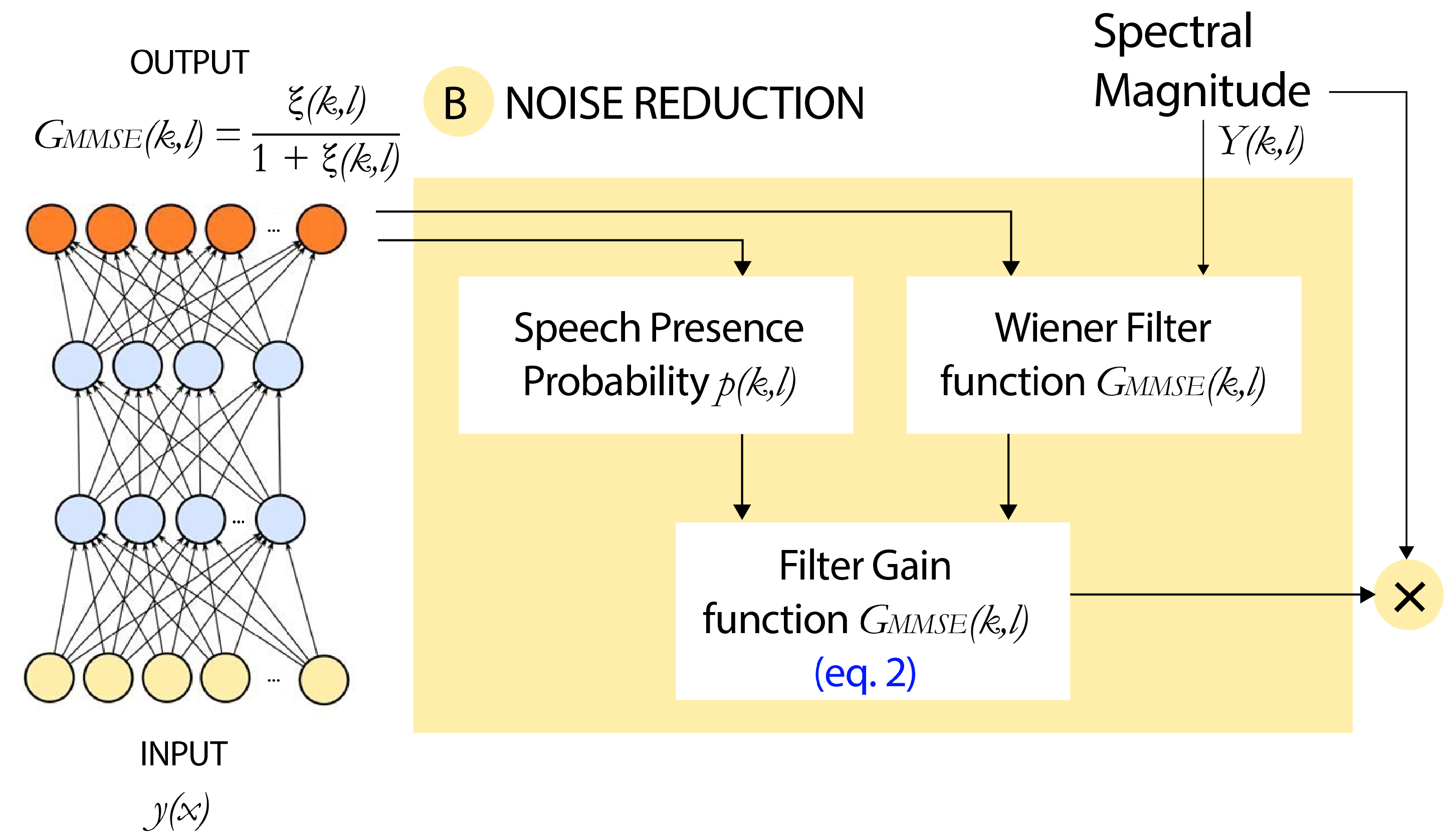
3. Proposal

This paper takes advantage of the data-driven paradigm behind deep learning for modeling the relationship between noise and clean data. We propose to obtain an estimate of the full term $G_{MMSE}(k,l)=\frac{\xi }{1+\xi }$, i.e., the Wiener filter directly from the noisy signal by means of a deep structured network. This term is subsequently used in the expression of the gain function of the optimally modified version of LSA according to Equations (4) and (6).

When the observed signal is barely noise affected, i.e., it is mostly clean, the dynamic range of the SNR can rise to ∞. In this case, the regression would be more sensitive to errors because there will be a huge amount of possible values to provide as result. However, as the $G_{MMSE}$ depends on the SNR (Equation (9)), high SNR conditions provoke high gain values $G_{MMSE}\to 1$, while low SNR conditions dump $G_{MMSE}\to 0$. This way, the dynamic range for the regression to obtain $G_{MMSE}$ would be bounded $[0,1]$, which is a more accurately achievable task for a deep structured network.

$$G_{MMSE}=\frac{1}{1+\frac{1}{SNR}}$$

(9)

Furthermore, the use of a deep structured network in this task was also motivated by the fact that we can implement a causal enhancement system. This means that as this is not necessarily dependent on future time frames, it can be employed in online applications. In addition, the network performs non-recursive estimations, which avoid the re-insertion of estimation errors from previous frames. The mentioned previous statistical SNR-estimators are usually based on recursive and causal schemes [9,13].

Figure 2 depicts the DL-based noise reduction method proposed. The deep structured network is trained in supervised mode with clean speech data and noise patterns through a standard data augmentation process. The goal of the network is to obtain an accurate estimate of the MMSE gain from the noisy signal. During training, in order to obtain this estimate, according to Equations (2) and (7), the network needs to know the PSD of the clean speech $P_x(k,l)$ and the PSD of the noise $P_d(k,l)$. We estimate those PSDs by means of the Welch method [29].

During inference, the input to the network is only the noisy signal $y\left(n\right)$. The $G_{MMSE}(k,l)$ delivered by the network is directly applied along with the speech presence probability term $p(k,l)$ to compute the final speech enhancement filter gain function $G(k,l)$ according to Equations (4) and (6). There are many ways of estimating the speech presence probability. Since the Wiener filter provides a value between 0 (when noise energy is much higher than the speech energy) and 1 (when the noise energy is much lower than the speech energy) we have directly used this term as an accurate estimate of the speech presence probability for each time instant and for each frequency bin. This way of estimating the presence of speech in the noisy signal is also appropriate in the sense that it does not require the use of estimates of the clean signal or the noise signal, avoiding the appearance of feedback loops that involve the speech enhancement gain function estimated by the method.

4. Architecture

For estimating the $G_{MMSE}$ we used a modified Wide-ResNet (WRN) architecture with multiple inputs based on 1-dimensional convolutions. The architecture was built on Pytorch toolkit. As the front end, we used a configuration of speech representations computed on a 25 ms Hamming window frame (overlap = 10 ms). For each frame segment, three types of acoustic feature vectors are computed and stacked to create a single input feature vector for the network: 512-dimensional FFT, 32 Mel filterbank, and 32 cepstral features. Finally, input data are normalized using the mean and variance of the training dataset.

During training, input features are generated on the fly. This way, in a single forward pass, the system computes the mask predictions for every t-f region and obtains the average loss to calculate the gradients. For this process, each audio in the training set is divided into segments of 2 seconds (200 frames). Then, the system creates a batch with 32 of these segments for training the network. During the evaluation, the inference of the mask is computed for the whole utterance in the evaluation set.

The architecture is composed of five blocks of WRN with an increasing number of channels. All the blocks are connected to the input features. Each block has four WRN, and only the first has kernel context in the convolutions as indicated in

Table 1. Description of the network dimensions of the architecture used for estimating $G_{MMSE}$. The dimension corresponds to the number of channels in the sequence of the processed frames.

Layer	Kernel Size	Dilation	Input Dim.	Output Dim.
Block 1 (×4 WRN)	7	3	512	256
Block 2 (×4 WRN)	5	3	512 + 256	512
Block 3 (×4 WRN)	3	2	512 + 512	1024
Block 4 (×4 WRN)	3	2	512 + 1024	2048
Block 5 (×4 WRN)	3	2	512 + 2048	2048
Output (Linear Layer)	-	-	512 + 2048	512

. The network employs causal convolutions such that only information from the past intervenes in the present result. For saving computations, we used groups in the convolutions. The AdamW algorithm was used to train the network [30,31] and PReLUs [32] as a parametric non-linearity. The cost function for a segment of contiguous frames is based on the mean square error (MSE).

5. Experimental Setup

To test the performance of the speech enhancement method proposed, the computation of speech quality measures on simulated speech samples was carried out.

5.1. Datasets

Data for DL training: We used 16 kHz sampled data from Timit (https://catalog.ldc.upenn.edu/LDC93S1 (accessed on 1 September 2022)) and Librispeech (http://www.openslr.org/12/ (accessed on 1 September 2022)) datasets in English, as well as some data in Spanish from Albayzin, Speechdatcar, Domolab, Tcstar, Mavir, and some hours of Spanish TV emissions for a total of approximately 120 h of clean speech. These data were augmented by adding randomly stationary and non-stationary noises from the Musan dataset [33], SNR = 0–30 dB, including music and speech, and scaling the time axis at the feature level.

Data for speech enhancement: We created a simulated noisy dataset with 11,976 speech utterances using clean read phrases in Spanish, phonetically balanced, from the laboratory sessions of the AV@CAR dataset [34]. The dataset is sampled at 16 kHz and includes 20 male and female speakers. The clean data were corrupted with different types of stationary and non-stationary additive noise:

• Babble: Noisy pattern from the talking of many people. It is a special case of non-stationary noise, very difficult to handle because it is highly correlated with the target voice since it is also voice.
• Traffic: Noise from the traffic at a random street, including cars, klaxon, street noise, etc.
• Cafe: Mixture of environmental noises in a cafe, including people talking, noise from cutlery, etc.
• Tram: Environmental noise in a tram station, including some stationary segments when the tram arrives.

In order to have a representation of several noise levels according to different scenarios of application, each noisy subset was evaluated at $SNR=0,5,10,15,20$ dB.

5.2. Speech Quality Measures

To evaluate the speech enhancement performance, the objective quality metric PESQ (perceptual evaluation of speech quality) [35] (from 0.5 to 4.5) is employed. STOI, short-time objective intelligibility [36], is used for objective intelligibility evaluation, where the intelligibility score is presented as a percentage. There are also results for quality metrics related to the MOS index. CBAK and COVL [37] are composite objective quality measures that provide a MOS from 1–5, where the first targets the background-noise intrusiveness, and the second target the overall signal quality. In all mentioned quality metrics, larger values indicate better speech quality.

Additionally, for evaluating the speech estimator, the level of noise reduction was analyzed by means of the SNR output level using the WADA algorithm [38]. The distortion of the enhanced signal was assessed by means of the log-likelihood ratio (also known as Itakura distance) (LLR) [39]. LLR represents the degree of discrepancy between the smoothed spectra of the target and reference signals, computed over the active speech segments of the linear prediction coefficients. For LLR, the closer the target feature to the reference, the lowest the spectral distortion; therefore, smaller values indicate better speech quality.

6. Results and Discussion

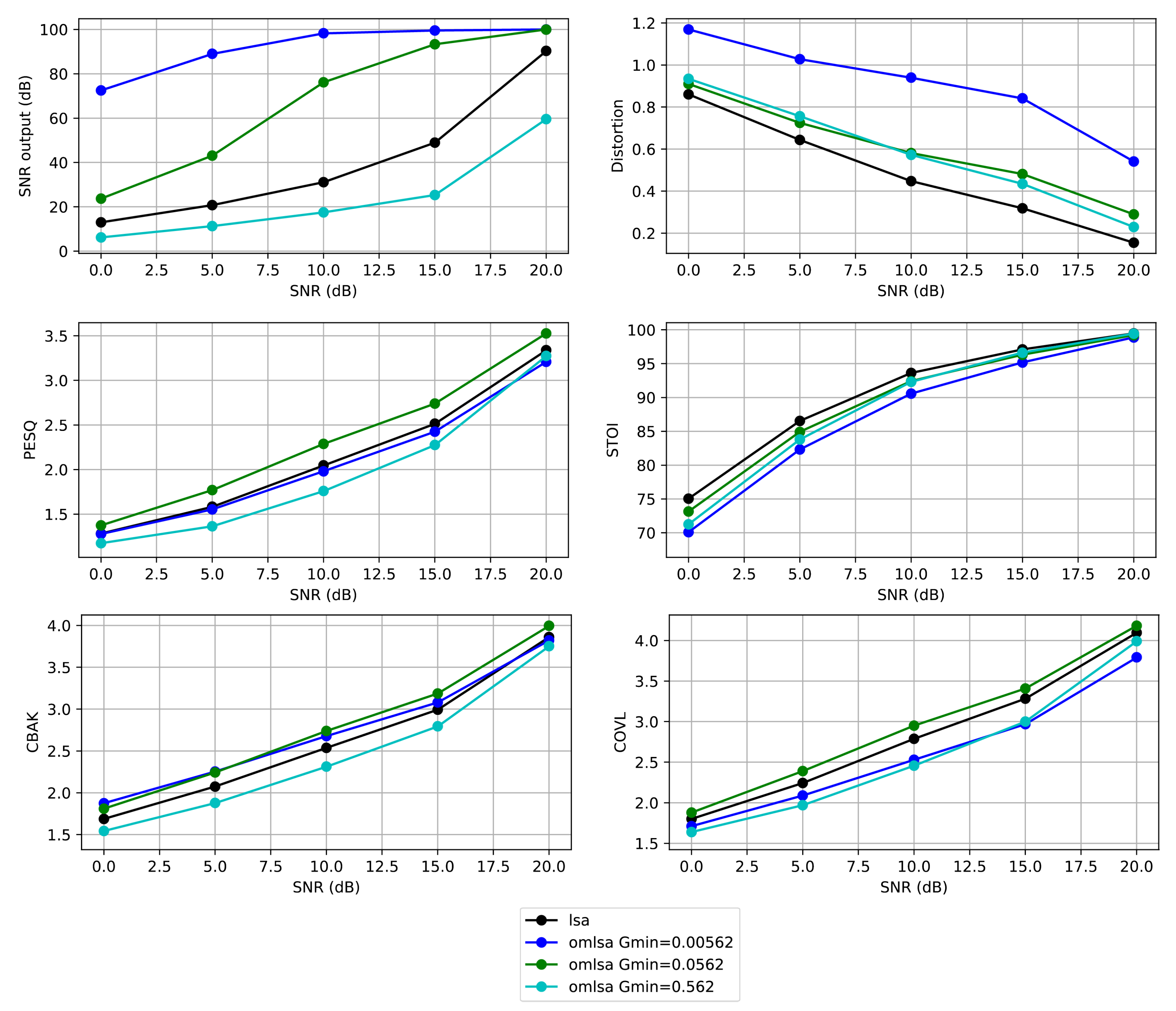
6.1. Evaluation of the Speech Estimator

This section consists of assessing the system performance using two speech estimators: LSA and OMLSA. The objective of this experiment is evaluating the impact of the SPP in the enhancement performance. OMLSA speech estimator applies the Wiener filter according to the spectral distribution of speech and silence. This is defined by a map of the probability of speech for the t-f regions, called speech presence probability (SPP) [24]. In this paper, the SPP feed from the same $G_{MMSE}$ obtained with the deep structured network. Then it is applied according to the $Gmin$ (Equation (6)), which is a boundary for the minimum gain that translates into a regulatory term for the strongest of the enhancement. The following experiment tests different values of $Gmin$ to evaluate its impact in the performance. On the other side, the LSA speech estimator does not use the SPP, and instead it directly employs the Wiener filter estimation as described in Equation (4).

Figure 3 shows the results of quality metrics for the speech estimation based on LSA and OMLSA with different $Gmin$ values. The variation among $Gmin$ values allows seeing the best trade-off between enhancement and distortion throughout the objective quality metrics. The highest SNR was obtained by the system using OMLSA with the lowest $Gmin$ (0.00562). However, in this case, the corresponding signal distortion is also highest among all. Conversely, the system based on LSA achieved the lowest signal distortion in terms of LLR, while the noise reduction is moderated since the SNR was in the middle of cases. The lowest SNR improvement was for $Gmin=0.562$ as expected, where the enhancement is slightly considering the noise dominant bins (see Equation (6)), so the signal remains very noisy. The desirable result is a reasonable trade-off between distortion and SNR level, where the SNR improvement indicates the noise reduction but at the same time, the signal distortion does not increase too much.

On the other side, the best performance for objective quality by PESQ was achieved by the system based on OMLSA with $Gmin=0.0562$. STOI results indicated that the intelligibility was not so variable among all conditions. The best performance was for moderated values of $Gmin$ and also for the system based on LSA. Note that these results are consistent with the system with lowest signal distortion. This is reasonable since we could expect better understanding when the speech is clearer and without robotic sounds. Finally, the best results for MOS-related metrics were again for the system based on OMLSA $Gmin=0.0562$. These results, together with a good improvement of SNR with moderated distortion, confirm that the best trade-off among all quality metrics evaluated belongs to the system based on OMLSA with $Gmin=0.0562$.

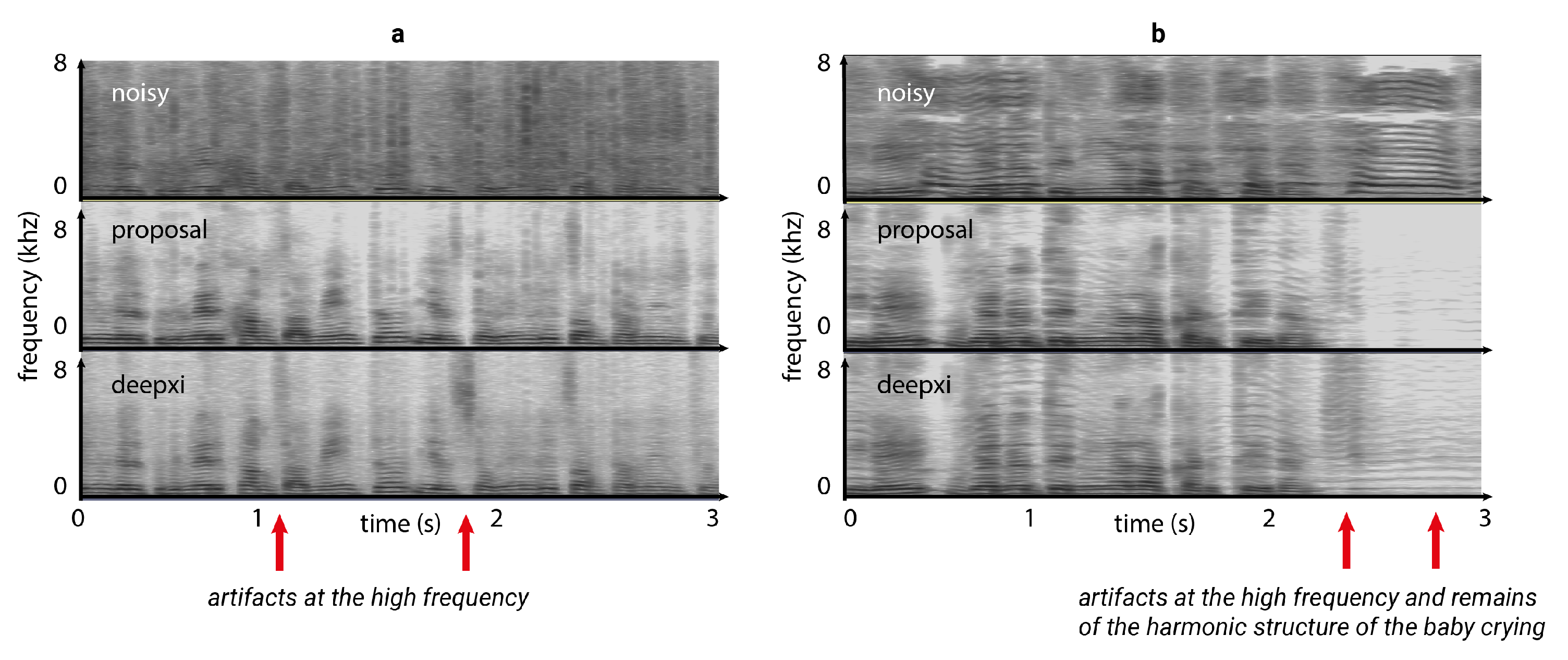
6.2. Preview of the Performance

In this section, there is a preview sketch of the system enhancement using spectrograms. Two audio examples from the dataset were used mixed with different noise types: baby crying and noise from call centers. There are more audio examples of the system enhancement, either on simulated or real noisy speech (http://dayanaribas.vivolab.es/DEMOenhancement/index.html (accessed on 1 September 2022)).

According to the previous section results, the system used was the one based on OMLSA with $Gmin=0.0562$. For comparison purposes, we used $Deepxi$ [22,23], a recent enhancement method from the state of the art with very competitive results (see the bench-marking table in the following link (https://github.com/anicolson/DeepXi (accessed on 1 September 2022)). Moreover, this method has common points with the proposal; for instance, it is also based on the combination of deep learning with classical speech estimators, and the version $DeepXi-ResNet\left(1.1c\right)$ uses Resnet with causal convolutions.

Figure 4a shows the spectrogram of an utterance corrupted with noise from a call center, while Figure 4b shows other speech sample mixed with the sound of a baby crying. In both examples, SNR = 5 dB and the speech is immersed into the noise, so it is difficult to distinguish the spectral structures of speech. Below the noisy speech are the spectrogram corresponding to the method proposed in this paper and the method for comparison purposes $deepxi$. At a glance, we appreciate that the spectrograms of both enhancement methods are very similar. In order to highlight some difference, we see that the structure of harmonics and the speech formants in example (a) are more defined with the method proposed than with $deepxi$, which spectrogram is softer. There are also some artifacts from the noisy speech (indicated with red arrows in the figure) that remain in the $deepxi$ spectrogram, while the method proposed was able to remove them. For example (b), the harmonic structure introduced by the crying is more pronounced in the spectrogram of $deepxi$. So when listening to this example, the baby crying is still a bit stronger in the background of the $deepxi$ sample than the proposal.

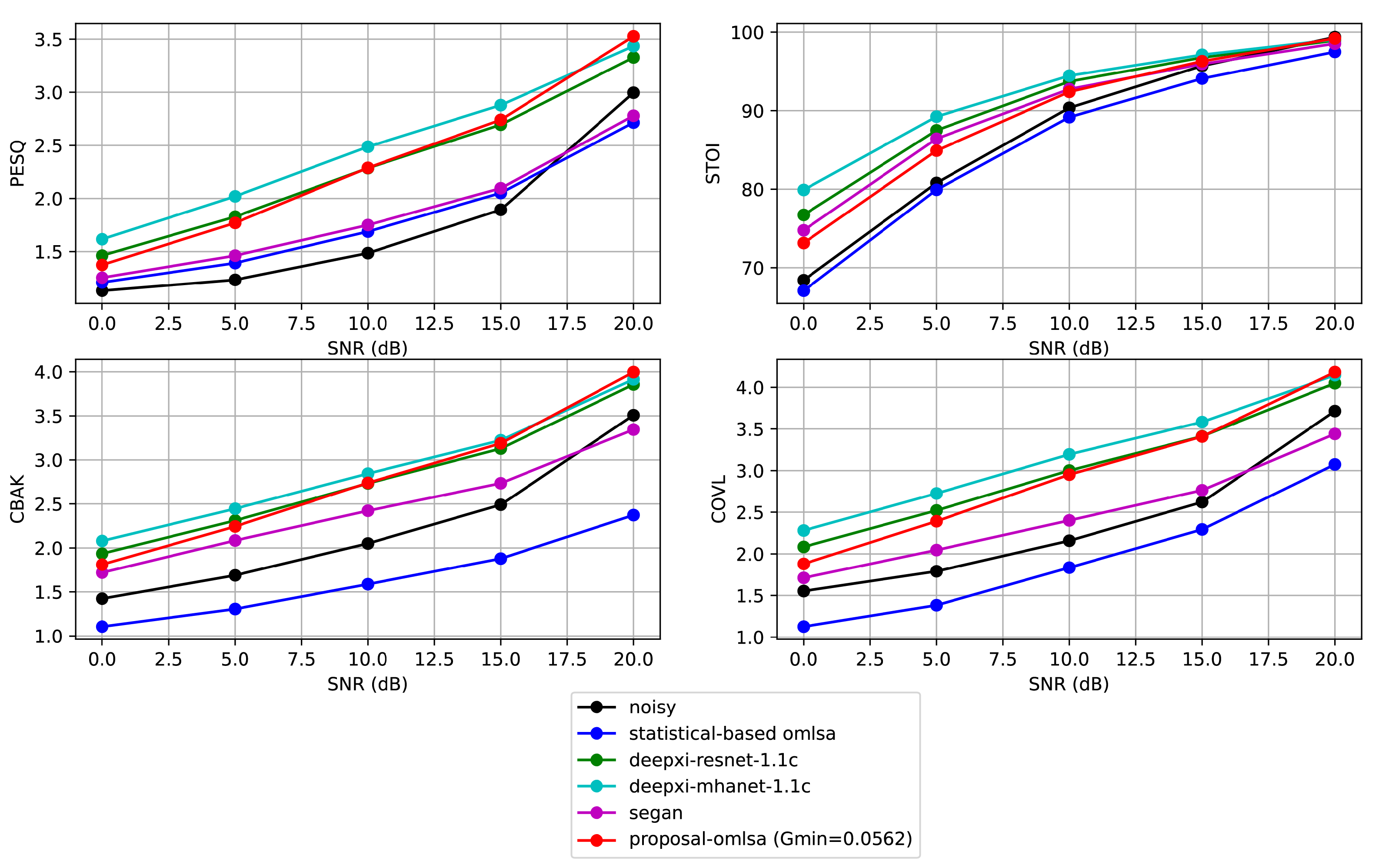
6.3. Objective Quality Metrics

This section presents the results of the objective quality metrics: PESQ, STOI, COVL, and CBAK. The black line is the reference that corresponds to the noisy speech, the blue line represents the statistical-based $omlsa$ method, and the red line is related to the $proposal$. For comparison purposes, we used three state-of-the-art DL-based SE methods $segan$ [40] and two $deepxi$ versions: resnet 1.1c [22] and mhanet 1.1c [23].

Figure 5 shows the results for objective quality metrics. Similar to the behavior shown by the spectrograms below, either the $proposal$, as all methods for comparison, achieved improvement of the objective quality concerning the noisy speech and also the statistical-based $omlsa$. $Segan$ obtained the most moderate results, except for intelligibility (STOI), where the performance is very similar for all methods evaluated. The method proposed and $deepxi$ achieved the best quality, with very similar values indeed. $deepxi$-$mhanet$-$1.1c$ achieved better values for PESQ and COVL. These metrics target the overall signal quality, so it is expected that both agree on the behavior. Note that the architecture behind this method employs multi-head attention (MHA), which is the most powerful architecture among all methods, so this result is expected to some extent. From the point of view of CBAK, $deepxi$ methods and the $proposal$ have almost the same background-noise intrusiveness, with a slight improvement of the proposal for $SNR$ > 10 dB. Note that in general, the difference between $deepxi$ and $proposal$ is slight. So, when listening to the signals enhanced, that difference among objective quality metrics is very hard to perceive in the practice.

In conclusion, the performance of the $proposal$ is very similar to the method $deepxi$-$resnet$-$1.1c$. However, the formulation of the $proposal$ is better suited for a deep learning solution because when targeting the estimation of the Wiener filter directly, it avoids practical issues, such as slow convergence. Additionally, as the estimated values are between 0 and 1, the same Wiener filter can be used as the spectral probability of the speech presence (SPP). This allows for employing the OMLSA-based speech estimator, instead of the LSA-based speech estimator used in both $deepxi$ methods evaluated. Previous results of Section 6.1 indicated that a suitable selection of $Gmin$ compensates for the distortion loss of the OMLSA-based speech estimator and outperforms the LSA-based speech estimator.

7. Conclusions

This paper proposed a deep learning method for estimating the Wiener filter for speech enhancement. Following the classical speech enhancement processing framework, this paper evaluated two spectral domain speech estimator algorithms: LSA and OMLSA. The obtained results indicated that despite LSA introducing very low distortion, the best trade-off among the speech enhancement, the signal distortion, and the objective quality metrics (PESQ, STOI, CBAK, COVL) was for the system based on OMLSA with $Gmin=0.0562$. Further studies on the combination of the DL-based Wiener filter estimation and other speech estimator algorithms would be analyzed in the next steps.

The method was evaluated for speech enhancement on a simulated noisy speech database and compared with state-of-the-art methods. Results showed that the proposal improves the statistical-based OMLSA, providing it with a robust version that accurately performs in simulated and real speech data. Regarding the state of the art, the proposal achieved better or similar performance. However, it proposes a better-suited formulation for a deep learning solution. This consists of directly targeting the estimation of the Wiener filter without the use of compensations for avoiding practical issues with the training convergence or the accuracy of the estimation. On the other side, the comparison with the state of the art shows that more sophisticated deep learning networks could produce more accurate estimation results, such as multi-head attention mechanisms and transformers. Audio examples of the enhancement performed in simulated and real noisy speech are available (http://dayanaribas.vivolab.es/DEMOenhancement/index.html (accessed on 1 September 2022)).

References

- Loizou, P.C. Speech Enhancement: Theory and Practice; CRC Press: New York, NY, USA, 2013. [Google Scholar]
- Hendriks, R.C.; Gerkmann, T.; Jensen, J. DFT-Domain Based Single-Microphone Noise Reduction for Speech Enhancement: A Survey of the State of the Art. Synthesis Lectures on Speech and Audio Processing; Morgan & Claypool: New York, NY, USA, 2013. [Google Scholar]
- Lim, J.S.; Oppenheim, A.V. Enhancement and bandwidth compression of noisy speech. Proc. IEEE 1979, 67, 1586–1604. [Google Scholar] [CrossRef]
- Boll, S. Suppression of acoustic noise in speech using spectral subtraction. IEEE Trans. Acoust. Speech Signal Process. 1979, 27, 113–120. [Google Scholar] [CrossRef]
- Ephraim, Y.; Malah, D. Speech enhancement using a minimum-mean square error short-time spectral amplitude estimator. IEEE Trans. Acoust. Speech Signal Process. 1984, 32, 1109–1121. [Google Scholar] [CrossRef]
- Ephraim, Y.; Malah, D. Speech enhancement using minimum-mean square log spectral amplitude estimator. IEEE Trans. Acoust. Speech Signal Process. 1985, 33, 443–445. [Google Scholar] [CrossRef]
- Breithaupt, C.; Martin, R. Analysis of the Decision-Directed SNR Estimator for Speech Enhancement with Respect to Low-SNR and Transient Conditions. IEEE Trans. Speech Audio Process. 2010, 19, 277–289. [Google Scholar] [CrossRef]
- Xia, B.Y.; Bao, C.C. Speech enhancement with weighted denoising Auto-Encoder. In Proceedings of the 14th Annual Conference of the International Speech Communication Association (Interspeech), Lyon, France, 25–29 August 2013; pp. 3444–3448. [Google Scholar]
- Xia, B.Y.; Bao, C.C. Wiener filtering based speech enhancement with Weighted Denoising Auto-encoder and noise classification. Speech Commun. 2014, 60, 13–29. [Google Scholar] [CrossRef]
- Wang, D.; Chen, J. Binary and ratio time-frequency masks for robust speech recognition. Speech Commun. 2006, 48, 1486–1501. [Google Scholar]
- Wang, D.; Chen, J. Supervised speech separation based on deep learning: An overview. IEEE/ACM Trans. Audio Speech Lang. Process. 2018, 26, 1702–1726. [Google Scholar] [CrossRef]
- Narayanan, A.; Wang, D.L. Ideal ratio mask estimation using deep neural networks for robust speech recognition. In Proceedings of the IEEE International Conference on Acoustic, Speech and Signal Processing (ICASSP), Vancouver, BC, Canada, 26–31 May 2013; pp. 7092–7096. [Google Scholar]
- Narayanan, A.; Wang, D.L. Investigation of speech separation as a front-end for noise robust speech recognition. IEEE Trans. Audio, Speech Lang. Process. 2014, 22, 826–835. [Google Scholar] [CrossRef]
- Healy, E.W.; Yoho, S.E.; Wang, Y.; Wang, D. An algorithm to improve speech recognition in noise for hearing-impaired listeners. J. Acoust. Soc. Am. 2013, 134, 3029–3038. [Google Scholar] [CrossRef]
- Healy, E.W.; Yoho, S.E.; Wang, Y.; Apoux, F.; Wang, D. Speech-cue transmission by an algorithm to increase consonant recognition in noise for hearing-impaired listeners. J. Acoust. Soc. Am. 2014, 136, 3325–3336. [Google Scholar] [CrossRef] [PubMed] [Green Version]
- Healy, E.W.; Yoho, S.E.; Chen, J.; Wang, Y.; Wang, D. An algorithm to increase speech intelligibility for hearing-impaired listeners in novel segments of the same noise type. J. Acoust. Soc. Am. 2015, 138, 1660–1669. [Google Scholar] [CrossRef] [PubMed]
- Healy, E.W.; Delfarah, M.; Johnson, E.; Wang, D. A deep learning algorithm to increase intelligibility for hearing-impaired listeners in the presence of a competing talker and reverberation. J. Acoust. Soc. Am. 2019, 145, 1378–1388. [Google Scholar] [CrossRef]
- Bolner, F.; Goehring, T.; Monaghan, J.; van Dijk, B.; Wouters, J.; Bleeck, S. Speech enhancement based on neural networks applied to cochlear implant coding strategies. In Proceedings of the ICASSP, Shanghai, China, 20–25 March 2016; pp. 6520–6524. [Google Scholar]
- Goehring, T.; Bolner, F.; Monaghan, J.; van Dijk, B.; Zarowski, A.; Bleeck, S. Speech enhancement based on neural networks improves speech intelligibility in noise for cochlear implant users. J. Hear. Res. 2017, 344, 183–194. [Google Scholar] [CrossRef] [PubMed]
- Goehring, T.; Keshavarzi, M.; Carlyon, R.P.; Moore, B.C.J. Using recurrent neural networks to improve the perception of speech in non-stationary noise by people with cochlear implants. J. Acoust. Soc. Am. 2019, 146, 705–708. [Google Scholar] [CrossRef]
- Zhang, Q.; Nicolson, A.; Wang, M.; Paliwal, K.K.; Wang, C. DeepMMSE: A Deep Learning Approach to MMSE-Based Noise Power Spectral Density Estimation. IEEE/ACM Trans. Audio Speech Lang. Process. 2020, 28, 1404–1415. [Google Scholar] [CrossRef]
- Nicolson, A.; Paliwal, K.K. Deep learning for minimum mean-square error approaches to speech enhancement. Speech Commun. 2019, 111, 44–45. [Google Scholar] [CrossRef]
- Nicolson, A.; Paliwal, K.K. On training targets for deep learning approaches to clean speech magnitude spectrum estimation. J. Acoust. Soc. Am. 2021, 149, 3273–3293. [Google Scholar] [CrossRef]
- Cohen, I.; Berdugo, B. Speech enhancement for non-stationary noise environments. Signal Process. 2001, 81, 2403–2418. [Google Scholar] [CrossRef]
- McAulay, R.J.; Malpass, M.L. Speech Enhancement using a Soft-Decision Noise Supression Filter. IEEE Trans. Acoust. Speech Signal Process. 1980, 28, 137–145. [Google Scholar] [CrossRef]
- Malah, D.; Cox, R.; Accardi, A. Tracking speech-presence uncertainty to improve speech enhancement in non-stationary noise environments. In Proceedings of the International Conference on Acoustics, Speech, and Signal Processing (ICASSP), Phoenix, AZ, USA, 15–19 March 1999. [Google Scholar]
- Hirsch, H.; Ehrlicher, C. Noise estimation techniques for robust speech recognition. In Proceedings of the International Conference on Acoustics, Speech, and Signal Processing (ICASSP), Detroit, MI, USA, 9–12 May 1995; pp. 153–156. [Google Scholar]
- Martin, R. Noise power spectral density estimation based on optimal smoothing and minimum statistics. IEEE Trans. Speech Audio Process. 2001, 9, 504–512. [Google Scholar] [CrossRef] [Green Version]
- Welch, P.D. The use of fast Fourier transforms for the estimation of power spectra: A method based on time averaging over short modified periodograms. IEEE Trans. Audio Electroacoust. 1967, 15, 70–73. [Google Scholar] [CrossRef]
- Kingma, D.P.; Ba, J.L. Adam: Amethod for stochastic optimization. In Proceedings of the 3rd International Conference on Learning Representations (ICLR), San Diego, CA, USA, 7–9 May 2015. [Google Scholar]
- Loshchilov, I.; Hutter, F. Fixing weight decay regularization in adam. arXiv 2017, arXiv:1711.05101. [Google Scholar]
- He, K.; Zhang, X.; Ren, S.; Sun, J. Delving deep into rectifiers: Surpassing human-level performance on imagenet classification. In Proceedings of the IEEE International Conference on Computer Vision, Santiago, Chile, 7–13 December 2015; pp. 1026–1034. [Google Scholar]
- Snyder, D.; Chen, G.; Povey, D. MUSAN: A Music, Speech, and Noise Corpus. arXiv 2015, arXiv:1510.08484v1. [Google Scholar]
- Ortega, A.; Sukno, F.; Lleida, E.; Frangi, A.; Miguel, A.; Buera, L.; Zacur, E. AV@CAR: A Spanish multichannel multimodal corpus for in-vehicle automatic audio-visual speech recognition. In Proceedings of the Language Resources and Evaluation (LREC), Reykjavik, Iceland, 26–31 May 2004; pp. 763–766. [Google Scholar]
- ITU-T Recommendation PESQ-862; Perceptual Evaluation of Speech Quality (PESQ): An Objective Method for End-to-End Speech Quality Assessment of Narrow-Band Telephone Networks and Speech Codecs. International Telecommunication Union (ITU): Geneva, Switzerland, 2001.
- Taal, C.H.; Hendriks, R.C.; Heusdens, R.; Jensen, J. A short-time objective intelligibility measure for time-frequency weighted noisy speech. In Proceedings of the 2010 IEEE International Conference on Acoustics, Speech and Signal Processing, Dallas, TX, USA, 14–19 March 2010; pp. 4214–4217. [Google Scholar] [CrossRef]
- Hu, Y.; Loizou, P.C. Evaluation of objective quality measures for speech enhancement. IEEE Trans. Audio Speech Lang. Process. 2007, 16, 229–238. [Google Scholar] [CrossRef]
- Chanwoo Kim, R.M.S. Robust Signal-to-Noise Ratio Estimation Based on Waveform Amplitude Distribution Analysis. In Proceedings of the 9th Annual Conference of the International Speech Communication Association (Interspeech), Brisbane, Australia, 22–26 September 2008; pp. 2598–2601. [Google Scholar]
- Loizou, P.C. Speech Quality Asssessment. In Multimedia Analysis, Processing and Communications; Springer: Berlin/Heidelberg, Germany, 2011; pp. 623–654. [Google Scholar]
- Pascual, S.; Bonafonte, A.; Serr, J. Segan: Speech enhancement generative adversarial network. In Proceedings of the 18th Annual Conference of the International Speech Communication Association (Interspeech), Stockholm, Sweden, 20–24 August 2017; pp. 3642–3646. [Google Scholar]