GLFormer: Global and Local Context Aggregation Network for Temporal Action Detection

Abstract

As the core component of video analysis, Temporal Action Localization (TAL) has experienced remarkable success. However, some issues are not well addressed. First, most of the existing methods process the local context individually, without explicitly exploiting the relations between features in an action instance as a whole. Second, the duration of different actions varies widely; thus, it is difficult to choose the proper temporal receptive field. To address these issues, this paper proposes a novel network, GLFormer, which can aggregate short, medium, and long temporal contexts. Our method consists of three independent branches with different ranges of attention, and these features are then concatenated along the temporal dimension to obtain richer features. One is multi-scale local convolution (MLC), which consists of multiple 1D convolutions with varying kernel sizes to capture the multi-scale context information. Another is window self-attention (WSA), which tries to explore the relationship between features within the window range. The last is global attention (GA), which is used to establish long-range dependencies across the full sequence. Moreover, we design a feature pyramid structure to be compatible with action instances of various durations. GLFormer achieves state-of-the-art performance on two challenging video benchmarks, THUMOS14 and ActivityNet 1.3. Our performance is 67.2% and 54.5% AP@0.5 on the datasets THUMOS14 and ActivityNet 1.3, respectively.

1. Introduction

In recent years, with the popularization of multimedia devices and the rapid development of the Internet, a dramatically increasing number of videos are produced every day, and relying on people to analyze videos has been far from meeting the actual needs. As a fundamental component of video content analysis technology, temporal action detection (TAD) has attracted more and more interest from industry and academia. The TAD task aims to predict the start/end boundaries and action categories for action instances as accurately as possible in the untrimmed video. TAD is mainly for public areas such as security surveillance, precision medicine, and intelligent manufacturing. It needs to collect a large amount of video data; a distributed storage platform that can detect copyright infringement is particularly important. In addition, there is still the threat of the raw video being forged and tampered with. One can refer to the content in [1,2] for further information.

As we all know, image classification and object detection have achieved impressive performance. Most of the previous works were inspired by object detection due to its macroscopic similarity to the temporal action detection task. Notable studies predominantly fall into three paradigms. First is the temporal convolution paradigm, whose representative works include SSAD [3], R-C3D [4], MGG [5], and A2net [6], stacking multiple 1D convolutions with a fixed kernel size to extract feature information. Another thread of work, such as [7,8,9], is tackling the TAD task in the form of evaluating frame-level action probabilities and combining consecutive frames through the watershed algorithm to generate proposals.

The third is a boundary-sensitive network, such as BSN [10] and BMN [11]. For each temporal location, predict the probabilities of whether it belongs to boundaries or actionness, then proposals are generated based on boundary probabilities. However, these approaches fall into a local trap; each temporal location is calculated independently as an isolated point, resulting in a lack of contextual connection and sensitivity to noise.

To solve the island problem, several works have attempted to establish long-range dependencies. PGCN [12] proposed exploiting the relations between proposals using graph convolution. BSN++ [13] optimizes the method that generated proposals only based on boundary probabilities, which designs a proposal relation block to explore the proposal–proposal relations. These methods belong to the local-then-global strategy, whose video-level prediction is achieved by following a post-processing step after the frame-level processing results. However, these works ignore the fact that the internal features of an action instance belong to a whole. Thus, this two-stage processing strategy will fragment the integrity. Inspired by Transformer’s success in NLP [14] and object detection [15], several recent works attempted to adopt the Transformer architecture to establish long-range dependencies, such as TadTR [16], RTD-Net [17], and ActionFormer [18].

We observed that action instances with various durations are randomly distributed in the original video. Therefore, if the Transformer structure is directly applied, there will be noise and multi-scale problems. To address these issues, we present the global and local context aggregation network (GLFormer). Compared with the other visual Transformer methods, we make three significant improvements to adapt to the TAD task. Firstly, to alleviate the noise issues while avoiding attention distraction caused by excessively long temporal ranges, we replace the original self-attention of Transformer with window self-attention. However, we are convinced that long-range dependencies are crucial for generating proposals. Thus, in order to exploit its advantages, the local self-attention module is followed by a lightweight global attention module as another branch. Lastly, to tackle the temporal multi-scale problem, we propose a parallel branch structure, adding a multi-scale local context module, which is parallel to the window self-attention module. Furthermore, the temporal feature pyramid is constructed by the temporal downsampling operation, and each level is regarded as a stage. The structure we design takes into account multi-scale local context, long-range dependencies, and global information, all of which complement each other. We conduct extensive ablation experiments on the THUMOS14 [19] and ActivityNet 1.3 [20] datasets to verify the effectiveness of our work. In summary, our main contributions are three-fold:

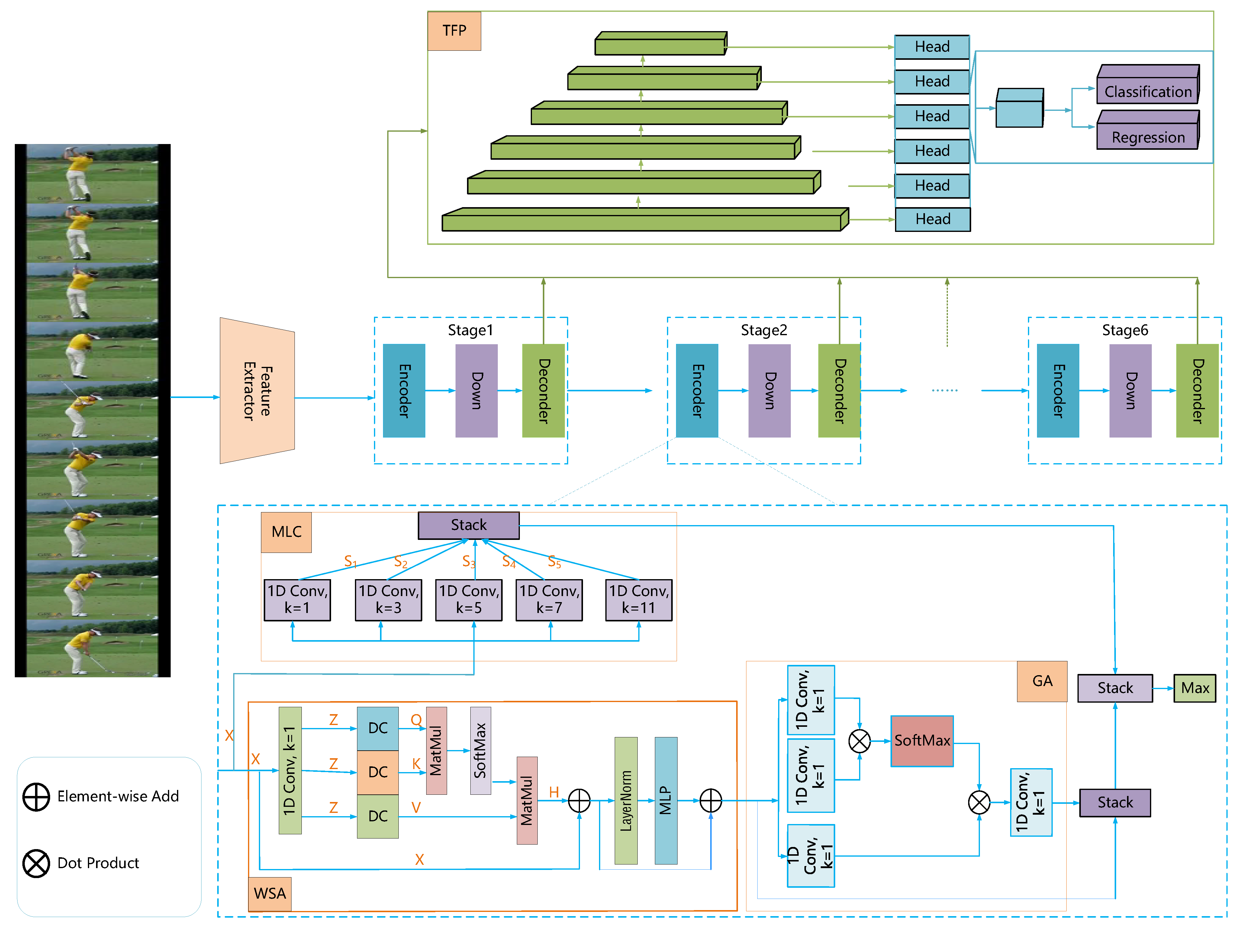
• We design a tandem structure with window self-attention followed by a lightweight global attention module, which can not only establish long-range dependencies, but also effectively avoid the introduction of noise.
• We add a multi-scale local context branch parallel to the window self-attention, forming a dual-branch structure. This stems from our desire to simultaneously take into account local context, long-range dependencies, and global information, which can help adaptively capture temporal context for temporal action detection.
• We design a feature pyramid structure to be compatible with action instances of various durations. Moreover, our network enables end-to-end training and achieves state-of-the-art performance on two representative large-scale human activity datasets, namely THUMOS14 and ActivityNet 1.3.

2. Related Work

2.1. Action Recognition

Like image recognition in the field of image analysis, as a fundamental task in video understanding areas, action recognition has been extensively investigated in recent years. Traditional methods such as MBH [21], HOF [22], and HOG [23] rely heavily on hand-designed ways to extract features. Inspired by the vast success of convolutional neural networks in the image domain, the current mainstream contains two categories: (a) The first is two-stream networks [24], which take RGB and optical flow as the input. The spatial stream captures the appearance features from the RGB image, while the temporal stream learns the motion information from dense optical flow. (b) The C3D network [25] obtains spatial–temporal feature information directly from the input video. A pre-trained action recognition model is usually used as a feature extractor for TAD tasks. By convention, we adopt I3D [26] pre-trained on the Kinetics-400 [27] dataset to generate the feature sequence as the input for our model.

2.2. Temporal Action Localization

Recent approaches in this task can be roughly divided into three categories: (1) The first is local-then-proposal; these methods, such as TAG [8], BSN [10], and R-C3D [4], first extract frame-level or snippet-level features and then generate proposals via action/boundary probabilities or the distance from the boundary. (2) Next is proposal-and-proposal; processing each proposal individually ignores the semantic relationship between proposals. PGCN [12] constructs a graph of proposals to explore the proposal–proposal relations. Complex videos may include overlapping, irregular, or non-sequential instances. AGT [28] proposes a novel Graph Transformer method to model the non-linear temporal structure using graph self-attention mechanisms. (3) The third is global-then-proposal, utilizing the global context in the sequence task. RTD-Net [17] and ActionFormer [18] adopt the Transformer structure, which helps to establish long-range dependencies. A summary of some recent work is shown in

Table 1. Summary of some representative temporal action detection methods.

Characteristic	Ref.	Year	mAP@0.5	Advantages	Limitations
Anchor-Based	RC3D [4]	ICCV-2017	28.9	The method adopts the 3D fully convolutional network and proposalwise pooling to predict the class confidence and boundary offset for each pre-specified anchor.	These methods require pre-defined anchors, which are inflexible for action instances with varying durations.
	TALNet [29]	CVPR-2018	42.8	The method proposes dilated convolutions and a multi-tower network to align receptive fields.
	GTAN [30]	CVPR-2019	38.8	The method learns a set of Gaussian kernels to dynamically predict the duration of the candidate proposal.
	PBRNet [31]	AAAI-2020	51.3	The method uses three cascaded modules to refine the anchor boundary.
Bottom-up	BSN [10]	ECCV-2018	36.9	The method predicts the probability of the start/end/action for each temporal location and then pairs the locations with higher scores to generate proposals.	These methods utilize the boundary probability to estimate the proposal quality, which are sensitive to noise and prone to local traps.
	BMN [11]	ICCV-2019	38.8	The method proposes an end-to-end framework to predict the candidate proposal and category scores simultaneously.
	BUTAL [32]	ECCV-2020	45.4	The method uses the potential relationship between boundary actionness and boundary probabilities to refine the start and end positions of action instances.
	BSN++ [13]	AAAI-2021	41.3	The method exploits proposal–proposal relation modeling and a novel boundary regressor to improve boundary precision.
Anchor-Free	MGG [5]	CVPR-2019	37.4	The method combines two complementary generators with different granularities to generate proposals from fine (frame) and coarse (instance) perspectives, respectively.	These methods directly localize action instances without predefined anchors, thus lacking the guidance of prior knowledge, resulting in easily missed action instances.
	A2Net [6]	TIP-20	45.5	This method combines the anchor-free and anchor-based methods.
	AFSD [33]	CVPR-2021	55.5	The method uses contrastive learning and boundary pooling to refine candidate proposals’ boundary.
	Actionr [18]	2022	65.6	This method introduces Transformer as the feature encoder.

.

2.3. Vision Transformer

Transformer was originally developed by [14] in the machine translation task. The core of Transformer is the self-attention architecture, which can transform one sequence into another sequence. Specifically, the output is computed as the weighted sum of the input features, where the weight is computed by a dot product at each temporal location. Therefore, Transformer can establish long-range dependencies. Recurrent neural networks such as RNN [34], LSTM [35], and GRU [36] have natural advantages in sequence modeling. However, in recent years, they have been gradually replaced by Transformers in many sequential tasks. Transformers have three key advantages: (1) the design of the parallel computing architecture breaks through the inherent serial properties of RNN models; (2) in the self-attention structure, the distance between any two temporal locations is one, which enables the model to remember longer-range dependencies’ information; (3) compared with the convolutional neural network (CNN), the Transformer model has a stronger interpretability. We only use the encoder part of the original Transformer on videos to explore the long-range dependencies.

3. Approach

3.1. Overall Architecture

An overview of our method is depicted in Figure 1. Our method consists of a stack of L = 6 stages, with the temporal length halved except for the first stage, thereby generating a temporal feature pyramid structure. All stages have an identical structure, which is used to aggregate multi-range context features. Moreover, every stage includes three modules: multi-scale local convolution (MLC), window self-attention (WSA), and global attention (GA).

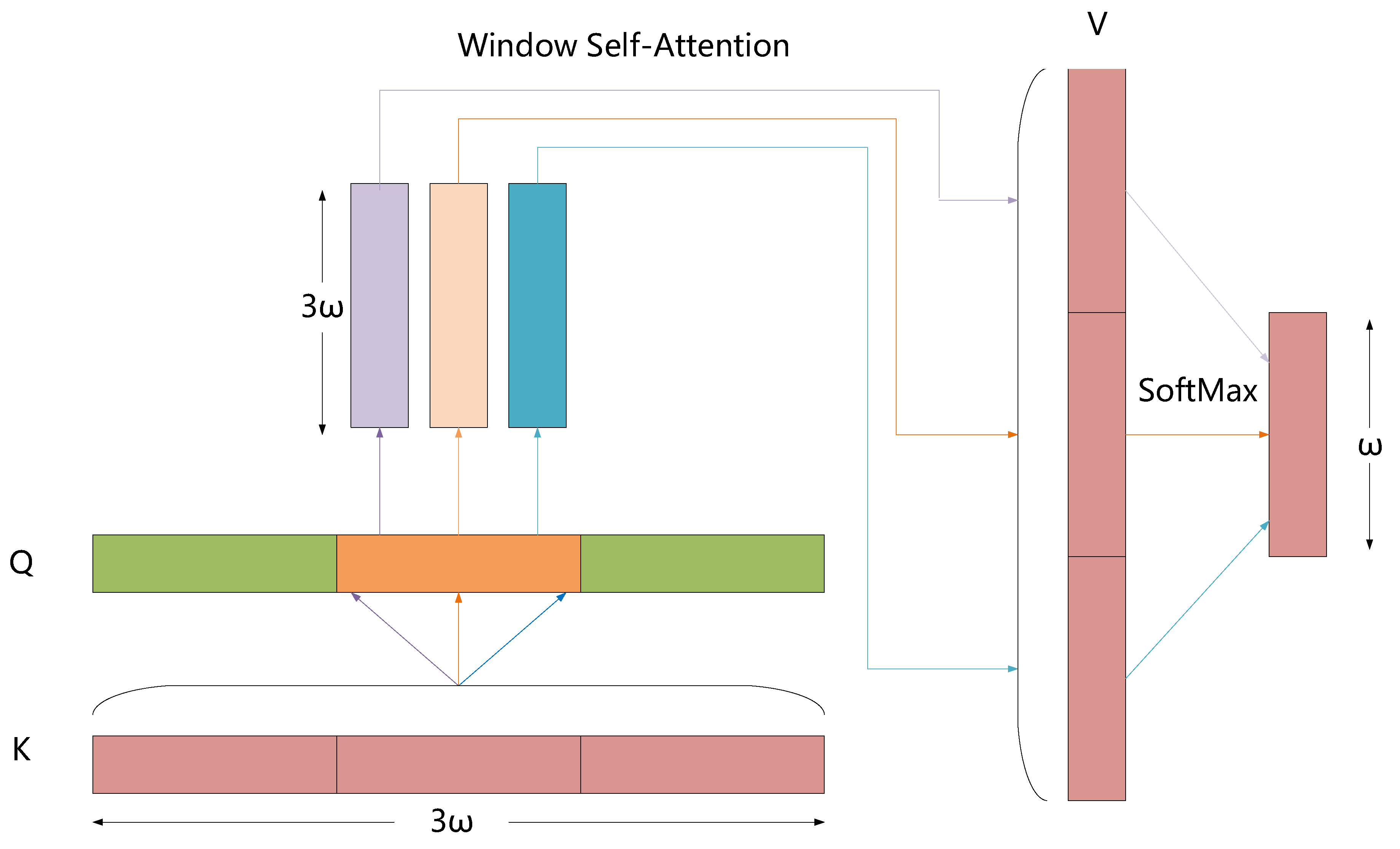
3.2. Window Self-Attention

Unlike the traditional way of directly using X = {$X_1,X_2,X_3,\cdots ,X_T$} as the input, we first use a 1D convolutional network to convert the dimension of the input X ∈$R^{T\times C}$ into the dimension we need $R^{T\times C}$→$R^{T\times D}$, where T denotes the temporal length and C and D represent the channel dimensions. This operation also contributes to the stability of the training process [37], represented as X = $\{X_1,X_2,X_3,\cdots ,X_T\}\stackrel{Conv1D}{⟹}$ Z = $\{Z_1,Z_2,Z_3,\cdots ,Z_T\}$.

The core part in the Transformer [14] network is the self-attention. We inserted a normalization block (Pre-LN [38]) before the self-attention block to remove the learning rate warm-up stage. In order to perform the attention function, the traditional way uses linear projection to generate values (V), queries (Q), and keys (k).These projections are parameter matrices with parameters $W_Q\in R^{D\times d_q}$, $W_K\in R^{D\times d_k}$, $W_V\in R^{D\times d_v}$, used to learn linear projections of features Z $\in R^{T\times D}$ to Q $\in R^{T\times d_q}$, K $\in R^{T\times d_k}$, V $\in R^{T\times d_v}$, where $d_q$, $d_k$, $d_v$ denote the channel dimensions. However, we found that it was beneficial to replace with 1D depthwise convolution (DC), which was implemented by using a layer 1D group convolution with a kernel size of 3 and group numbers the same as the channel dimension. A main advantage of the self-attention block is the ability to capture global-range dependencies across the full sequence. However, this advantage comes at the cost of introducing noise and increasing computation when the temporal length exceeds a certain range. Inspired by the local self-attention from Longformer [39] and Actionformer [18], we adopted the window self-attention mechanism to get rid of the impact of a long sequence. For features at location i ∈ [1, T], we call it a token. This gives a sequence of arbitrary length, and our window self-attention pattern uses a fixed-range attention around each token. For a specified window size $\omega$, we evenly divided the input sequence into T$/\omega$ attention chunks. A chunk is denoted as ${\Phi }_i=\{{\varphi }_i,{\phi }_i,{\psi }_i\}$, i $\in [1,T/\omega ]$, where ${\varphi }_i$${\phi }_i$ and ${\psi }_i$ are keys ($K_i$), queries ($Q_i$), and values ($V_i$) of the feature sequence separately. For a chunk region ${\Psi }_i\in [t_s,t_e]$, we denote its region $R_K=[t_s,t_e]$, $R_Q=[t_s-\omega ,t_e+\omega ],R_V=[t_s-\omega ,t_e+\omega ]$ separately, where $\omega =t_e-t_s$ (see Figure 2). In this way, the range of attention is limited within a chunk. At stage j ∈ [1, L], the range of attention is j × $\omega$. Stacking multiple window self-attention layers naturally integrates short-, medium-, and long-range features, which is beneficial to multi-scale prediction. V, Q, and K are computed as

$$Q=Dw\_Conv1D\left(Z\right),group=in\_channel,k=3$$

(1)

$$V=Dw\_Conv1D\left(Z\right),group=in\_channel,k=3$$

(2)

$$K=Dw\_Conv1D\left(Z\right),group=in\_channel,k=3$$

(3)

We used projection Q and $K-V$ pairs to compute the window attention of each chunk, and the weight assigned to $V\in R^{3\omega \times d_v}$ is computed by matrix multiplication $Q{\mathbf{K}}^{\top }$, where ${\mathbf{K}}^{\top }$ represents the transpose of K, $Q\in R^{\omega \times d_q}$, $K\in R^{3\omega \times d_k}$. The attention of the full sequence is obtained via the temporal sliding window approach with window size 3$\omega$ and stride $\omega$. The result of window self-attention is calculated as a weighted sum of V:

$$H=Attention(Q,K,V)=[Softmax(\frac{Q_i{\mathbf{K}}_{\mathbf{i}}^{\top }}{\sqrt{d_q}})V_i{]}_1^{T/\omega },H\in R^{T\times D}$$

(4)

In order to avoid the problem of gradient disappearance due to the dot product growing large in magnitude, we scaled the dot product S by $1/\sqrt{d_q}$. Similar to Transformer’s multi-head attention, we used h = 4 parallel attention heads [$H_1,H_2,H_3,H_4$], where the dimension of each head is $d_q$ = $d_k$ = $d_v$ = D/h = 256.

$$YW=MultiHead(Q,K,V)=Concat(H_1,H_2,H_3,H_4),YW\in R^{T\times D}$$

(5)

3.3. Global Attention

In the actual processing, a fundamental problem for the window self-attention method is how to set the window size. If it is too long, it goes against the original intention of the design. On the contrary, it may not cover the full context of the longer action instance, resulting in insufficient information. Inspired by Transformer [14] and non_local [40], the window self-attention module is followed by a lightweight global attention module. We define the operation in our network as:

$$YG={[\frac{1}{\mathcal{N}\left(Y{W}_i\right)}\sum _{\forall j}\mathcal{F}(\theta \left(Y{W}_i\right),\varphi \left(Y{W}_i\right))\mathcal{H}\left(Y{W}_i\right)]}_1^T,1\le i,j\le T,YW\in R^{T\times D}$$

(6)

where

$$\begin{array}{c}\hfill \theta \left(Y{W}_i\right)=Conv1D\left(Y{W}_i\right),\varphi \left(Y{W}_j\right)=Conv1D\left(Y{W}_j\right),\mathcal{H}\left(Y{W}_j\right)=Conv1D\left(Y{W}_j\right)\end{array}$$

(7)

The linear projection functions $\theta$, $\varphi$, and $\mathcal{H}$ are implemented in three independent layers of 1D convolutions with kernel size 1. where i ∈ [1, T], j ∈ [1, T]. The pairwise function $\mathcal{F}$ is utilized to calculate the dot product between arbitrary feature vectors, which represent the similarity relationship. This similarity score is normalized by $\mathcal{N}\left(Y{W}_i\right)$ = ${\sum }_{\forall j}$$\mathcal{F}$$\left(\theta \left(Y{W}_j\right)\right),\varphi \left(Y{W}_j\right)$, used to prevent the dot product from becoming too large.

3.4. Multi-Scale Local Convolution

The Transformer structure is mainly used to establish long-range dependencies, and capturing local context is its shortcoming. However, the convolutional neural network (CNN) is adept at capturing local features, and combining convolution kernels of various sizes can simultaneously extract multi-scale local features. Based on this concept, we propose a multi-scale local convolution (MLC) module parallel with the window self-attention module to capture multi-scale local context information. MLC consists of multiple independent 1D convolutions with different kernel sizes, the kernel size with a typical choice $d_1<\cdots <d_n$, which defines increasingly larger receptive fields. Figure 1 shows a sketch of MLC. As seen, MLC is composed of five different 1D convolutions, and the size of the kernels ranges between d, d ∈ {1, 3, 5, 7, 11}. The feature maps ${\left\{M_k\right\}}_{k=1}^5$ are directly concatenated into a dense aggregated intermediate feature map $[M_1,M_2,M_3,M_4,M_5]$. The five features have the same dimension. Then, we used the max pooling operation along the temporal dimension to generate multi-scale local contextual features $YM\in R^{T\times D}$.

3.5. Temporal Feature Pyramid

Inspired by resnet [41] and FPN [42], we designed a temporal feature pyramid by stacking multiple pyramid levels to enhance the expressiveness of the network. Specifically, we applied a temporal downsampling operation at each pyramid level to accommodate action instances with various durations, where the downsampling rate is between d, d ∈ {1, 2, 2, 2, 2, 2}. Each pyramid level consists of MLC, WSA, and GA modules, and the output of each module is independent. Therefore, the network has the ability to capture local, window, and global range features simultaneously. In order to aggregate these features, a MAX operator is adopted along the temporal dimension, which is used to filter out the strongest features. The aggregation strategy can be expressed as

$$\begin{array}{cc}\hfill & \hfill {\overline{S}}_{\tau }=Y{W}^{\tau }\parallel Y{G}^{\tau }\parallel Y{M}^{\tau },\tau =1,2,3,\cdots ,L\hfill \end{array}$$

(8)

$$\begin{array}{cc}\hfill & \hfill {\tilde{S}}_{\tau }=MAX\left({\overline{S}}^{\tau }\right),\tau =1,2,3,\cdots ,L\hfill \end{array}$$

(9)

$$\begin{array}{cc}\hfill & \hfill S_{\tau }=\downarrow \left({\tilde{S}}_{\tau }\right),\tau =2,3,\cdots ,L,S_{\tau }\in {\mathbf{R}}^{T/2(\tau -1)\times D}\hfill \end{array}$$

(10)

where ∥ denotes the concatenation operation, $\tau$ represents the pyramid level, and ↓ represents the downsampling operation, which is implemented with a 1D convolution with a stride of 2. Finally, we combined the results of all stages and obtained the temporal feature pyramid set S = {$S_1,S_2,\cdots ,S_6$}. We designed two lightweight prediction branches with the same structure, but independent of each other, for action classification and boundary regression, respectively. This structure consists of three layers of 1D convolution with a kernel size of 3. We considered every location i ∈ [1, T] in the sequence as an action instance candidate. For the classification branch, a sigmoid function was followed to predict the probability $C_t^i$ of action categories. Similar to the regression branch, in order to ensure that the distance ($d_t^s,d_t^e$) to the left and right boundary is a positive number, a Relu activation function is attached at the end.

4. Training and Inference

4.1. Loss Function

The output of our network includes the start/end boundary $\left(d_t^s,d_t^e\right)$ and class probability $C_t$, and we used the following loss function to optimize the model:

$$\mathcal{L}={\mathcal{L}}_{cls}+\lambda {\mathcal{L}}_{reg}$$

(11)

where $\lambda$ is a hyper-parameter, used to adjust the weight of the classification and regression losses, and we treated these two losses equally and set $\lambda$ = 1. Our classification loss uses the focal loss [43] function, which can effectively solve the problem of the imbalance between the foreground and background

$${\mathcal{L}}_{cls}=\frac{1}{T_j}\sum _{t=0}^{T_j}\sum _{i=0}^N-{\alpha }_{\mathrm{t}}^i{\left(1-p_{\mathrm{t}}^i\right)}^{\gamma }log\left(p_{\mathrm{t}}^i\right)$$

(12)

where

$$\begin{array}{cc}\hfill p_{\mathrm{t}}^i& \hfill =\left\{\begin{array}{cc}\hfill C_t^i\hfill & \hfill \mathrm{if}{y}_t^i=1,i=0,1,2,\cdots ,N\hfill \\ \hfill 1-C_t^i\hfill & \hfill \mathrm{otherwise},i=0,1,2,\cdots ,N\hfill \end{array}\right.\hfill \end{array}$$

(13)

$$\begin{array}{cc}\hfill {\alpha }_{\mathrm{t}}^i& \hfill =\left\{\begin{array}{cc}\hfill \alpha \hfill & \hfill \mathrm{if}{y}_t^i=1,i=0,1,2,\cdots ,N\hfill \\ \hfill 1-\alpha \hfill & \hfill \mathrm{otherwise},i=0,1,2,\cdots ,N\hfill \end{array}\right.\hfill \end{array}$$

(14)

In the above, class label $y_t\in R^N$, $y_t^i\in \{0,1\}$, indicates whether the temporal location t ∈ [1, T] belongs to action ($y_t^i=1$) or background ($y_t={\left\{0\right\}}_{i=0}^N$), the predicted classification score $C_t$ = {$C_t^1,C_t^2,\cdots ,C_t^N$}. $T_j$ is the length of the full sequence in the j-th stage, and N represents the total number of action categories. $\alpha$ and $\gamma$ are hyper-parameters, which are specified as 0.25 and 2 in the experiments. ${\mathcal{L}}_{reg}$ is the intersection over union (IOU) loss [44] between predicted boundaries ${\widehat{\Omega }}_t=\left({\widehat{\theta }}_t,{\widehat{\xi }}_t\right)$ and the corresponding ground truth ${\Omega }_t=\left({\theta }_t,{\xi }_t\right)$:

$${\mathcal{L}}_{reg}=\frac{1}{T_p}\sum _t\mathbb{I}\left(y_t\ge 1\right)\left(1-\frac{|{\widehat{\Omega }}_t\cap {\Omega }_t|}{|{\widehat{\Omega }}_t\cup {\Omega }_t|}\right)$$

(15)

where $T_p$ represents the total number of positive samples. The function $\mathbb{I}$ is used to indicate that the location t ∈ [1, T] is inside ($\mathbb{I}=1$) or outside ($\mathbb{I}=0$) an action instance.

4.2. Inference

During inference, we fed the feature sequences into the network and obtain the predictions $A_t^j$ = ${(C_t^i,d_t^s,d_t^e)}_0^L$ for every temporal location t across all pyramid levels, where i $\in R^N$ and j $\in R^L$ represent the action category and pyramid level, respectively. For the t-th temporal location in the j-th level, the predicted action instance is represented by

$$C_t^i=argmax{C}_t,s_t=t-d_t^s,s_t=t+d_t^e$$

(16)

where $s_t$ and $e_t$ are the left and right offsets of an action instance and $C_t^i$ represents the category of the action instance. Finally, the predicted results from all locations are merged, and we performed Soft-NMS [45] and obtained the final outputs.

5. Experiments

5.1. Datasets and Settings

We evaluated our model on two widely used large-scale datasets, THUMOS14 [19] and ActivityNet 1.3 [20]. THUMOS14 contains 20 sport categories and consist of three parts: training, validation, and testing sets. Among all the videos, the training set with no temporal annotations was used for action recognition. Following previous research [3,6,12], we trained our model on the validation set including 213 untrimmed videos and evaluated the performance on the test set including 200 untrimmed videos. ActivityNet 1.3 is composed of 19,994 videos, which contain 200 action categories, and the dataset is divided into training, testing, and validation subsets in a ratio of 2:1:1.

5.2. Evaluation Metrics

To compare with existing methods, we used official evaluation metrics, the mean average precision (mAP) at different temporal intersection over unions (tIoUs) and the average mAP to evaluate the performance on the two datasets. On THUMOS14, the tIoU thresholds were chosen from [0.3:0.1:0.7], which focuses on the performance of mAP@0.5. On Activitynet v1.3, the tIoU thresholds were selected from 0.5, 0.75, 0.95, which pays more attention to the results of mAP@avg [0.5:0.1:0.95]. Each video in THUMOS14 contains more than 15 short-duration action instances, and each video in Activitynet v1.3 contains an average of 1.7 long-duration action instances. Thus, the two datasets use different evaluation metrics.

5.3. Implementation Details

THUMOS14: In order to extract spatial–temporal features from THUMOS14, we used a two-stream inflated 3D ConvNet (I3D) [26] module pre-trained on the Kinetics-400 [27] dataset. We sampled 16 consecutive RGB and optical-flow with an overlap rate of 75% as clips, which were respectively input to the I3D network, and extracted features of dimension 512 × 2 at the first fully connected layer. Then, the output features of the two-stream network were concatenated to obtain the input features of our model. According to the evaluation method, the mean average precision (mAP) with an IoU threshold {0.3, 0.4, 0.5, 0.6, 0.7} was the evaluation metric used on THUMOS-14. We used Adam [46] to optimize the network and set the batch size, initial learning rate, and total epoch number as 2, ${10}^{-4}$, and 50, respectively.

ActivityNet 1.3: We adopted an R(2+1)D model to extract features from ActivityNet 1.3 pre-trained on the TSP [47] dataset. We sampled 16 consecutive frames with a stride of 16 as clips (i.e., non-overlapping clips). Following [10,18], the length of the sequence was rescaled into a fixed length of 128 using linear interpolation. According to the evaluation method, a mAP with IoU threshold {0.5, 0.75, 0.95} and an average mAP [0.5:0.05:0.95] were the evaluation metrics used on ActivityNet 1.3. We used Adam to optimize the network and set the batch size, initial learning rate, and total epoch number as 16, ${10}^{-3}$, and 15, respectively.

Our method was implemented based on PyTorch 1.1, Python 3.8, and CUDA 11.6. We conducted experiments with one NVIDIA GeForce RTX 3090 GPU, Intel i5-10400 CPU, and 128 G memory.

5.4. Comparison with State-of-the-Art Methods

THUMOS14: We compared our model with several recent state-of-the-art methods including one-stage, two-stage, and Transformer models on the THUMOS14 dataset.

Table 2. Comparison with the state-of-the-art (THUMOS14), measured by the mAP at different tIoU thresholds and the average mAP in {0.3, 0.4, 0.5,0.6,0.7}; the best results are in bold.

Method	Year	Backbone	mAP@0.3	mAP@0.4	mAP@0.5	mAP@0.6	mAP@0.7	mAP@avg
SCNN [50]	CVPR16	C3D	36.3	28.7	19.0	10.3	5.3	19.9
RC3D [2]	ICCV17	C3D	44.8	35.6	28.9	-	-	-
SSAD [3]	ACM17	TSN	43.0	35.0	24.6	-	-	-
TALNet [29]	CVPR18	I3D	53.2	48.5	42.8	33.8	20.8	39.8
BSN [10]	ECCV18	TSN	53.5	45.0	36.9	28.4	20.0	36.8
MGG [5]	CVPR19	I3D	53.9	46.8	37.4	29.5	21.3	37.8
PGCN [12]	ICCV19	I3D	60.1	54.3	45.5	33.5	19.8	42.6
BMN [11]	ICCV19	TSN	56.0	47.4	38.8	29.7	20.5	36.8
A2Net [6]	TIP20	I3D	58.6	54.1	45.5	32.5	17.2	41.6
GTAD [51]	CVPR20	TSN	54.5	47.6	40.2	30.8	23.4	39.3
BCGNN [52]	ECCV20	TSN	57.1	49.1	40.4	31.2	23.1	40.2
CSA [53]	ICCV21	TSN	64.4	58.0	49.2	38.2	27.8	47.5
AFSD [33]	CVPR21	I3D	67.3	62.4	55.5	43.7	31.1	52.0
ContextLoc [49]	ICCV21	I3D	68.3	63.8	54.3	41.8	26.2	50.9
TBOS [54]	CVPR21	C3D	63.2	58.5	54.8	44.3	32.4	50.6
RefactorNet [55]	CVPR2022	I3D	70.7	65.4	58.6	47.0	32.1	54.8
ActionFormer [18]	2022	I3D	75.5	72.5	65.6	56.6	42.7	62.6
BCNet [56]	AAAI22	I3D	71.5	67.0	60.0	48.9	33.0	56.1
RCL [57]	CVPR22	TSN	70.1	62.3	52.9	42.7	30.7	51.7
AES [58]	CVPR22	SF R50	69.4	64.3	56.0	46.4	34.9	54.2
GLFormer(Ours)		I3D	75.9	72.6	67.2	57.2	41.8	62.9

summarizes the performance. It can be seen intuitively that our model outperformed all previous methods, establishing the new state-of-the-art of 67.2% mAP@0.5 on THUMOS14. In particular, our model achieved an improvement of 11.7% (from 55.5% to 67.2%) on mAP@0.5 and 10.9% (from 52.0% to 62.9%) on the average mAP ([0.3:0.1:0.7]) compared with AFSD [33], which is currently the best-performing one-stage detector. We outperformed MUSES [48], which is the strongest two-stage competitor by 10.3% (from 56.9% to 67.2%) on mAP@0.5 and 9.5% on the average mAP (from 53.4% to 62.9%). Moreover, our model achieved up to 1.6% (from 65.6% to 67.2%) on mAP@0.5 and 0.3% (from 62.6% to 62.9%) on the average mAP over the Transformer method [16], which is the current state-of-the-art method in TAD tasks. The excellent performance proved that for TAD, simultaneous modeling of local multi-scale features and long-range temporal dependencies can effectively improve its performance.

ActivityNet 1.3: The performances on the ActivityNet 1.3 dataset are shown in

Table 3. Comparison with the state-of-the-art (ActivityNet 1.3), measured by the mAP at different tIoU thresholds, as well as the average mAP in [0.5:0.1:0.95]; the best results are in bold.

Method	Year	mAP@0.5	mAP@0.75	mAP@0.95	mAP@avg
PGCN [12]	ICCV19	48.3	33.2	3.3	31.1
BMN [11]	ICCV19	50.1	34.8	8.3	33.9
PBRNet [31]	AAAI20	54.0	35.0	9.0	35.0
GTAD [51]	CVPR20	50.4	34.6	9.0	34.1
AFSD [33]	CVPR21	52.4	35.3	6.5	34.4
ContextLoc [49]	ICCV21	56.0	35.2	3.6	34.2
MUSES [48]	CVPR21	50.0	35.0	6.6	34.0
ActionFormer [18]	2022	53.5	36.2	8.2	35.6
BCNet [56]	AAAI22	53.2	36.2	10.6	35.5
RCL [57]	CVPR22	51.7	35.3	8.0	34.4
AES [58]	CVPR22	50.1	35.8	10.5	35.1
GLFormer(Ours)		54.5	37.7	7.6	36.3

. On the average mAP, GLFormer reached an mAP of 36.3%, which is 0.7% higher than the current state-of-the-art of 35.6% by ActionFormer [18]. Our method achieved 37.7% mAP@0.75, outperforming all previous methods by at least 1.5%. GLFormer achieved 54.5% mAP@0.5, but did not perform as well as the previous method ContextLoc [49] (54.5% vs. 56.0%), but outperformed it on other evaluation metrics. Our method achieved 7.6% mAP@0.95 and had no advantage over other methods. Considering that the evaluation index mAP@avg is the average result of multiple tight tIoUs (such as tIoU = 0.95), it requires higher accuracy, so the performance of 36.3% is also commendable. This demonstrates the effectiveness and generalizability of fusing multi-scale context and long-range features.

6. Ablation Experiments

Here, in order to validate the various design decisions, we discuss the contributions from several key modules. All ablation experiments were performed on THUMOS14.

6.1. Effectiveness of WSA Module

By comparing the first and second rows in

Table 4. Ablation study on the window size in WSA. We report the mAP at tIoU from 0.3 to 0.7 and the average mAP in [0.3,0.4,0.5,0.6,0.7] on THUMOS14.

Projection Method	Window Size	mAP@0.3	mAP@0.4	mAP@0.5	mAP@0.6	mAP@0.7	mAP@avg
Conv1D	9	75.9	72.6	67.2	57.2	41.8	62.9
linear	9	75.1	71.9	65.5	55.8	43.1	62.3
Conv1D	4	75.6	72.3	65.7	56.6	42.3	62.5
Conv1D	6	76.0	72.8	66.4	56.1	42.2	62.7
Conv1D	12	75.2	72.2	65.5	55.7	42.0	62.2
Conv1D	18	76.1	73.1	66.9	56.6	42.1	62.9
Conv1D	full	75.5	72.8	65.8	55.8	42.0	62.4

, we found it beneficial to replace the linear projection approach of the traditional Transformer model with a 1D depthwise convolution to project the queries, keys, and values. The results showed that when using the 1D depthwise convolution, the mAP at tIoU 0.5 and the average mAP increased by 0.9% and 0.5%, respectively. This indicates that choosing an appropriate projection approach can help improve the performance of the TAL task. Observed in the third row, we evaluated the effect of the choice of the window size on the results. We can find that increasing the window size from 4 to 9 had an improvement (from 65.7% to 67.2% on mAP@0.5), while the performance dropped from 67.2% to 65.8% after continuing to increase the window size to the full sequence. The features located in the deep layers of the network are already highly abstracted, and simple linear projection may over-reorganize the channel features, resulting in insufficient feature distinguishability. The 1D group convolution prevents the features between groups from interfering with each other, and it learns independent expression patterns, which is beneficial to enhance the distinguishability of features. Setting the window size too small will damage the integrity of the information, while setting the window size too large will distract the attention and introduce irrelevant information.

6.2. Effectiveness of MLC Module

To discuss the effectiveness of the MLC module, we compared two settings: (1) WSA + GA module; (2) MLC + WSA + GA module. MLC is a multi-branch structure, and each branch consists of a layer of 1D convolution with different kernel sizes.

Table 5. Ablation study on the kernel size in MLC. √ indicates whether MLC contains the 1D convolution with corresponding kernel size or not, respectively.

Method	k = 1,3	k = 5,7	k = 9	k = 11	k = 13	k = 15	mAP@0.5	mAP@avg
WSA + GA							65.9	62.0
WSA + GA + MLC	√						66.5	62.9
WSA + GA + MLC	√	√					65.4	62.0
WSA + GA + MLC	√	√	√	√			66.2	62.3
WSA + GA + MLC	√	√	√				65.6	62.0
WSA + GA + MLC	√	√		√			67.2	62.9
WSA + GA + MLC	√	√			√		65.6	62.1
WSA + GA + MLC	√	√				√	65.3	62.2

shows the comparison results on the THUMOS14 test set. It can be seen that MLC + WSA + GA had a +1.1% mAP@0.5 improvement compared to only using the WSA + GA module, suggesting that the MLC module can provide complementary information with WSA + GA. As the number of branches increases, the accuracy further increases, with only a small increase in the model parameters. However, when using a larger kernel size (k_s = 13), the effectiveness of MLC seems to become weaker (−1.4% in mAP@0.5). Further expanding the kernel size (e.g., k_s = 15) leads to greater performance degradation. Multi-scale local features play an important role in enriching the feature details, but the range of the temporal receptive field must be controlled within a certain range. Beyond a certain range, the module’s attention is distracted, not only being unable to capture long-range features, but also unable to focus on the local context.

6.3. Effectiveness of GA Module

We validated the design of the GA module in Figure 1 by comparing three settings: (1) WSA + MLC module; (2) follow a GA after WSA; (3) follow multiple GAs after WSA. We compare the performance with or without the GA module in

Table 6. Ablation study of different GA settings on THUMOS14 in terms of mAP(%)@tIoU.

Method	mAP@0.3	mAP@0.4	mAP@0.5	mAP@0.6	mAP@0.7	mAP@avg
WSA + MLC	75.4	72.5	66.1	56.0	42.1	62.4
WSA + MLC + GA	75.9	72.6	67.2	57.2	41.8	62.9
WSA + MLC + 2GA	75.3	72.1	66.0	56.2	43.0	62.5
WSA + MLC + 3GA	75.4	72.5	66.1	56.3	42.8	62.6

. The result clearly shows that with a GA, the performance improves by 1.1% mAP@0.5. This experiment demonstrated that the GA was beneficial to make the localization precise. However, when we replaced a single GA module with two or three GAs, the performance dropped by 1.2% and 1.1% mAP@0.5, respectively. Using a GA module can help improve performance, indicating that only considering local features is not conducive to the model capturing sufficient features, especially for instances with a long duration. While noise may be introduced, the benefits are greater. Stacking more than two GA modules will amplify the noise in a cumulative manner, negating the benefits of capturing global features.

6.4. Module Complementarity

In order to study the relationship between the three modules of WSA (medium-range), MLC (short-range), and GA (long-range), we compared different combinations of these modules, and the results are presented in

Table 7. Ablation study of complementarity on THUMOS14 in terms of mAP(%)@tIoU.

Method	mAP@0.3	mAP@0.4	mAP@0.5	mAP@0.6	mAP@0.7	mAP@avg
WSA	75.5	72.4	65.8	56.0	41.4	62.2
WSA + GA	75.4	72.0	65.9	55.3	41.1	62.3
WSA + MLC	75.4	72.5	66.1	56.0	42.1	62.4
WSA + MLC + GA	75.9	72.6	67.2	57.2	41.8	62.9

. Just using the WSA module alone, the performance was 65.8% mAP@0.5, which is the strongest contributor to our model’s performance. Combined with MLC or GA, the performance improved by 0.3% and 0.1%, respectively. When we used these three modules together, the result were 67.2% mAP@0.5, which proves that the three modules have a complementary relationship. The MLC module is responsible for capturing multi-scale local contextual information. The WSA module and the following lightweight GA module can not only establish long-range dependencies, but also effectively avoid introducing noise. The three modules work together to enable the network to adaptively capture action instances with randomly varying durations.

6.5. Temporal Feature Pyramid

The temporal feature pyramid is used to accommodate action instances with various durations. In our experiments, different numbers of levels were tried, and the performance are listed in

Table 8. Ablation study of different channel settings on THUMOS14 in terms of mAP(%)@tIoU.

Levels	Channels	mAP@0.3	mAP@0.4	mAP@0.5	mAP@0.6	mAP@0.7	mAP@avg	GFLOPs
4	1024	74.1	69.7	61.3	50.2	36.5	58.4	37.5
5	1024	74.2	71.2	63.9	53.8	38.8	60.4	38.3
6	1024	75.9	72.6	67.2	57.2	41.8	62.9	38.8
7	1024	75.4	72.0	65.9	55.3	41.9	62.1	39.0
6	256	75.2	72.4	65.0	55.1	42.7	60.1	33.9
6	512	75.1	71.6	65.6	56.1	42.6	62.2	35.2
6	2048	75.7	72.4	66.0	56.1	42.5	62.5	50.2
6	4096	75.1	72.3	65.6	55.0	42.5	62.1	90.2

. We can observe that the performance became progressively better as the levels increased, with the six-level pyramid achieving the best result on mAP@0.5 and the average mAP, while using more levels did not result in better performance; this is due to more redundant candidates being involved. In Table 8, we also show the effectiveness of different numbers of channels on the performance. The initial number of channels was set to 256, and increasing the number of channels to 1024 can help improve the performance (from 65.0% to 67.2%). However, when continuing to increase the number of channels to 4096, the performance dropped from 67.2% to 65.6%. The number of channels is directly related to the expressiveness of the network. On the one hand, the low feature dimension will have difficulty providing sufficient information, making it difficult for the network to distinguish instances with a high similarity. On the other hand, for high-dimensional features, performing linear projection operations on highly abstract features not only increases the computational complexity, but also causes network overfitting.

6.6. Temporal Downsampling Module

For each pyramid level, we used a 1D convolution with a stride of 2 (except for the first level, which is 1) to reduce the temporal resolution. In addition, we also tried other downsampling methods, including average pooling and max pooling, and compared their results with this method. The performance is summarized in

Table 9. Ablation study of different downsampling operations on THUMOS14 in terms of mAP(%)@tIoU.

Method	mAP@0.3	mAP@0.4	mAP@0.5	mAP@0.6	mAP@0.7	mAP@avg
Max pooling	75.7	72.3	66.3	57.3	43.1	62.9
Avg pooling	75.5	72.0	66.0	55.6	42.1	62.3
stride = 2	75.9	72.6	67.2	57.2	41.8	62.9

. Among all temporal downsampling modes, the 1D convolution operation achieved the best performance, showing a 1.2% and 0.9% advantage for mAP@0.5 against average pooling and maximum pooling respectively. For max pooling and avg pooling, the cost of losing some feature information will be paid when reducing the time series dimension. However, the convolution with a stride of 2 reduces the dimension while not only retaining the features completely, but also enhancing the expressiveness of the network.

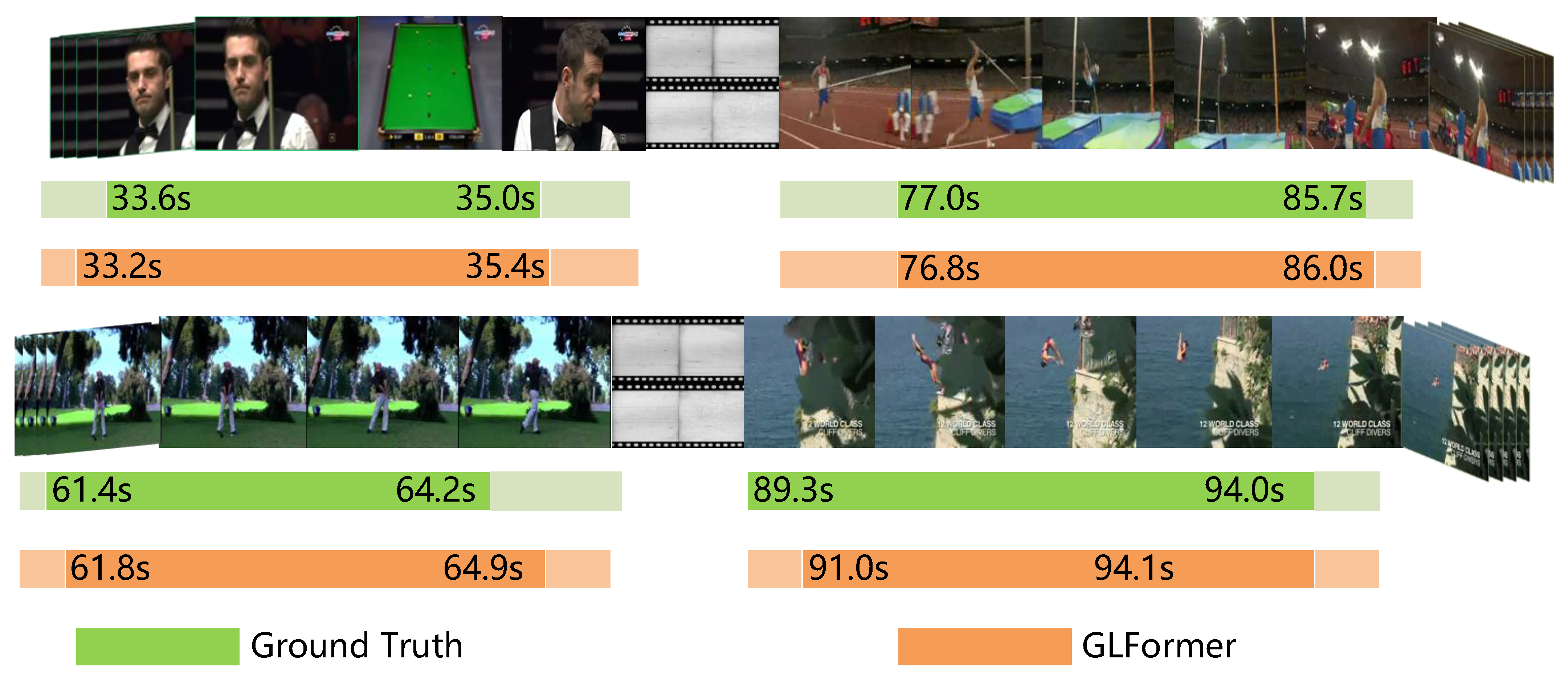
6.7. Visualization Results

We visualize four proposals generated by GLFormer, which include short, medium, and long action instances, and compare them with the ground truth in Figure 3. These four action instance samples are from the THUMOS14 dataset. The visualizations indicate that our results match the corresponding ground truth well even for short and long action instances.

7. Conclusions

In this paper, we introduced GLFormer for temporal action detection (TAD). This network takes advantage of multi-scale 1D convolution, global attention, and window self-attention to learn rich contexts for action classification and boundary prediction. Furthermore, taking into account action instances with various durations, an important component of our network is the temporal feature pyramid, which is achieved by using a 2× downsampling between successive stages. The experimental evaluation shows that our model achieves state-of-the-art performance on the human activity datasets THUMOS14 and ActivityNet 1.3. Overall, this work highlights the importance of aggregating features with different ranges of attention and shows that window self-attention is an effective means to model longer-range temporal context in complex activity videos.

Discussion: Although great achievements have been made in temporal action detection, there still remain many shortcomings that need further improvement: (i) manually labeling data results in excessive human and material investment, combining supervised learning with semi-supervised or even unsupervised learning; (ii) exploring effective post-processing methods to improve boundary positioning accuracy; (iii) the traditional TV-1 algorithm is inefficient and occupies storage space, which is replaced by the deep learning algorithm to realize the end-to-end processing process; (iv) real-world action instances are often dynamic and random (exploring effective methods to model nonlinear video sequence features); (v) adding data preprocessing steps to improve the quality of the raw data, such as the clutter effect, illumination effect, and complex scenarios.

References

1. Kumar, R.; Tripathi, R.; Marchang, N.; Srivastava, G.; Gadekallu, T.R.; Xiong, N.N. A secured distributed detection system based on IPFS and blockchain for industrial image and video data security. J. Parallel Distrib. Comput. 2021, 152, 128–143. [Google Scholar] [CrossRef]
2. Javed, A.R.; Jalil, Z.; Zehra, W.; Gadekallu, T.R.; Suh, D.Y.; Piran, M.J. A comprehensive survey on digital video forensics: Taxonomy, challenges, and future directions. Eng. Appl. Artif. Intell. 2021, 106, 104456. [Google Scholar] [CrossRef]
3. Lin, T.; Zhao, X.; Shou, Z. Single shot temporal action detection. In Proceedings of the 25th ACM International Conference, Mountain View, CA, USA, 23–27 October 2017; pp. 988–996. [Google Scholar]
4. Xu, H.; Das, A.; Saenko, K. R-c3d: Region convolutional 3d network for temporal activity detection. In Proceedings of the IEEE International Conference on Computer Vision, Venice, Italy, 22–29 October 2017; pp. 5783–5792. [Google Scholar]
5. Liu, Y.; Ma, L.; Zhang, Y.; Liu, W.; Chang, S.F. Multi-granularity generator for temporal action proposal. In Proceedings of the IEEE/CVF Conference on Computer Vision and Pattern Recognition, Long Beach, CA, USA, 15–20 June 2019; pp. 3604–3613. [Google Scholar]
6. Yang, L.; Peng, H.; Zhang, D.; Fu, J.; Han, J. Revisiting anchor mechanisms for temporal action localization. IEEE Trans. Image Process. 2020, 29, 8535–8548. [Google Scholar] [CrossRef] [PubMed]
7. Shou, Z.; Chan, J.; Zareian, A.; Miyazawa, K.; Chang, S.F. Cdc: Convolutional-de-convolutional networks for precise temporal action localization in untrimmed videos. In Proceedings of the IEEE Conference on Computer Vision and Pattern Recognition, Honolulu, HI, USA, 21–26 July 2017; pp. 5734–5743. [Google Scholar]
8. Xiong, Y.; Zhao, Y.; Wang, L.; Lin, D.; Tang, X. A pursuit of temporal accuracy in general activity detection. arXiv 2017, arXiv:1703.02716. [Google Scholar]
9. Yuan, Z.; Stroud, J.C.; Lu, T.; Deng, J. Temporal action localization by structured maximal sums. In Proceedings of the IEEE Conference on Computer Vision and Pattern Recognition, Honolulu, HI, USA, 21–26 July 2017; pp. 3684–3692. [Google Scholar]
10. Lin, T.; Zhao, X.; Su, H.; Wang, C.; Yang, M. Bsn: Boundary sensitive network for temporal action proposal generation. In Proceedings of the European Conference on Computer Vision (ECCV), Munich, Germany, 8–14 September 2018; pp. 3–19. [Google Scholar]
11. Lin, T.; Liu, X.; Li, X.; Ding, E.; Wen, S. Bmn: Boundary-matching network for temporal action proposal generation. In Proceedings of the IEEE/CVF International Conference on Computer Vision, Seoul, Korea, 27 October–2 November 2019; pp. 3889–3898. [Google Scholar]
12. Zeng, R.; Huang, W.; Tan, M.; Rong, Y.; Zhao, P.; Huang, J.; Gan, C. Graph convolutional networks for temporal action localization. In Proceedings of the IEEE/CVF International Conference on Computer Vision, Seoul, Korea, 27 October–2 November 2019; pp. 7094–7103. [Google Scholar]
13. Su, H.; Gan, W.; Wu, W.; Qiao, Y.; Yan, J. Bsn++: Complementary boundary regressor with scale-balanced relation modeling for temporal action proposal generation. arXiv 2020, arXiv:2009.07641. [Google Scholar]
14. Vaswani, A.; Shazeer, N.; Parmar, N.; Uszkoreit, J.; Jones, L.; Gomez, A.N.; Kaiser, Ł.; Polosukhin, I. Attention is all you need. In Proceedings of the Advances in Neural Information Processing Systems 30 (NIPS 2017), Long Beach, CA, USA, 4–9 December 2017; pp. 5998–6008. [Google Scholar]
15. Dosovitskiy, A.; Beyer, L.; Kolesnikov, A.; Weissenborn, D.; Zhai, X.; Unterthiner, T.; Dehghani, M.; Minderer, M.; Heigold, G.; Gelly, S.; et al. An image is worth 16 × 16 words: Transformers for image recognition at scale. arXiv 2020, arXiv:2010.11929. [Google Scholar]
16. Liu, X.; Wang, Q.; Hu, Y.; Tang, X.; Bai, S.; Bai, X. End-to-end temporal action detection with transformer. arXiv 2021, arXiv:2106.10271. [Google Scholar] [CrossRef] [PubMed]
17. Tan, J.; Tang, J.; Wang, L.; Wu, G. Relaxed transformer decoders for direct action proposal generation. In Proceedings of the IEEE/CVF International Conference on Computer Vision, Montreal, QC, Canada, 10–17 October 2021; pp. 13526–13535. [Google Scholar]
18. Zhang, C.; Wu, J.; Li, Y. ActionFormer: Localizing Moments of Actions with Transformers. arXiv 2022, arXiv:2202.07925. [Google Scholar]
19. Idrees, H.; Zamir, A.R.; Jiang, Y.G.; Gorban, A.; Laptev, I.; Sukthankar, R.; Shah, M. The THUMOS challenge on action recognition for videos “in the wild”. Comput. Vis. Image Underst. 2017, 155, 1–23. [Google Scholar] [CrossRef]
20. Zhao, Y.; Zhang, B.; Wu, Z.; Yang, S.; Zhou, L.; Yan, S.; Wang, L.; Xiong, Y.; Lin, D.; Qiao, Y.; et al. Cuhk & ethz & siat submission to activitynet challenge 2017. arXiv 2017, arXiv:1710.08011. [Google Scholar]
21. Dalal, N.; Triggs, B.; Schmid, C. Human detection using oriented histograms of flow and appearance. In Proceedings of the European Conference on Computer Vision, Graz, Austria, 7–13 May 2006; pp. 428–441. [Google Scholar]
22. Chaudhry, R.; Ravichandran, A.; Hager, G.; Vidal, R. Histograms of oriented optical flow and binet-cauchy kernels on nonlinear dynamical systems for the recognition of human actions. In Proceedings of the 2009 IEEE Conference on Computer Vision and Pattern Recognition, Miami, FL, USA, 20–25 June 2009; pp. 1932–1939. [Google Scholar]
23. Dalal, N.; Triggs, B. Histograms of oriented gradients for human detection. In Proceedings of the 2005 IEEE Computer Society Conference on Computer Vision and Pattern Recognition (CVPR’05), San Diego, CA, USA, 20–26 June 2005; Volume 1, pp. 886–893. [Google Scholar]
24. Simonyan, K.; Zisserman, A. Two-stream convolutional networks for action recognition in videos. In Proceedings of the Advances in Neural Information Processing Systems 27 (NIPS 2014), Montréal, QC, Canada, 8 December 2014; pp. 568–576. [Google Scholar]
25. Tran, D.; Bourdev, L.; Fergus, R.; Torresani, L.; Paluri, M. Learning spatiotemporal features with 3d convolutional networks. In Proceedings of the IEEE International Conference on Computer Vision, Santiago, Chile, 7 December 2015; pp. 4489–4497. [Google Scholar]
26. Carreira, J.; Zisserman, A. Quo vadis, action recognition? A new model and the kinetics dataset. In Proceedings of the IEEE Conference on Computer Vision and Pattern Recognition, Honolulu, HI, USA, 21–26 July 2017; pp. 6299–6308. [Google Scholar]
27. Kay, W.; Carreira, J.; Simonyan, K.; Zhang, B.; Hillier, C.; Vijayanarasimhan, S.; Viola, F.; Green, T.; Back, T.; Natsev, P.; et al. The kinetics human action video dataset. arXiv 2017, arXiv:1705.06950. [Google Scholar]
28. Nawhal, M.; Mori, G. Activity graph transformer for temporal action localization. arXiv 2021, arXiv:2101.08540. [Google Scholar]
29. Chao, Y.W.; Vijayanarasimhan, S.; Seybold, B.; Ross, D.A.; Deng, J.; Sukthankar, R. Rethinking the faster r-cnn architecture for temporal action localization. In Proceedings of the IEEE Conference on Computer Vision and Pattern Recognition, Salt Lake City, UT, USA, 18–23 June 2018; pp. 1130–1139. [Google Scholar]
30. Long, F.; Yao, T.; Qiu, Z.; Tian, X.; Luo, J.; Mei, T. Gaussian temporal awareness networks for action localization. In Proceedings of the IEEE/CVF Conference on Computer Vision and Pattern Recognition, Long Beach, CA, USA, 15–20 June 2019; pp. 344–353. [Google Scholar]
31. Liu, Q.; Wang, Z. Progressive boundary refinement network for temporal action detection. In Proceedings of the AAAI Conference on Artificial Intelligence, New York, NY, USA, 7–12 February 2020; Volume 34, pp. 11612–11619. [Google Scholar]
32. Zhao, P.; Xie, L.; Ju, C.; Zhang, Y.; Wang, Y.; Tian, Q. Bottom-up temporal action localization with mutual regularization. In Proceedings of the European Conference on Computer Vision, Glasgow, UK, 23–28 August 2020; pp. 539–555. [Google Scholar]
33. Lin, C.; Xu, C.; Luo, D.; Wang, Y.; Tai, Y.; Wang, C.; Li, J.; Huang, F.; Fu, Y. Learning salient boundary feature for anchor-free temporal action localization. In Proceedings of the IEEE/CVF Conference on Computer Vision and Pattern Recognition, Nashville, TN, USA, 19–25 June 2021; pp. 3320–3329. [Google Scholar]
34. Mikolov, T.; Karafiát, M.; Burget, L.; Cernockỳ, J.; Khudanpur, S. Recurrent neural network based language model. In Proceedings of the Interspeech, Chiba, Japan, 26–30 September 2010; Volume 2, pp. 1045–1048. [Google Scholar]
35. Hochreiter, S.; Schmidhuber, J. Long short-term memory. Neural Comput. 1997, 9, 1735–1780. [Google Scholar] [CrossRef] [PubMed]
36. Chung, J.; Gulcehre, C.; Cho, K.; Bengio, Y. Empirical evaluation of gated recurrent neural networks on sequence modeling. arXiv 2014, arXiv:1412.3555. [Google Scholar]
37. Xiao, T.; Singh, M.; Mintun, E.; Darrell, T.; Dollár, P.; Girshick, R. Early convolutions help transformers see better. Adv. Neural Inf. Process. Syst. 2021, 34, 30392–30400. [Google Scholar]
38. Xiong, R.; Yang, Y.; He, D.; Zheng, K.; Zheng, S.; Xing, C.; Zhang, H.; Lan, Y.; Wang, L.; Liu, T. On layer normalization in the transformer architecture. In Proceedings of the International Conference on Machine Learning, Vienna, Austria, 12–18 July 2020; pp. 10524–10533. [Google Scholar]
39. Zhang, P.; Dai, X.; Yang, J.; Xiao, B.; Yuan, L.; Zhang, L.; Gao, J. Multi-scale vision longformer: A new vision transformer for high-resolution image encoding. In Proceedings of the IEEE/CVF International Conference on Computer Vision, Montreal, QC, Canada, 10–17 October 2021; pp. 2998–3008. [Google Scholar]
40. Wang, X.; Girshick, R.; Gupta, A.; He, K. Non-local neural networks. In Proceedings of the IEEE Conference on Computer Vision and Pattern Recognition, Salt Lake City, UT, USA, 18–23 June 2018; pp. 7794–7803. [Google Scholar]
41. He, K.; Zhang, X.; Ren, S.; Sun, J. Deep residual learning for image recognition. In Proceedings of the IEEE Conference on Computer Vision and Pattern Recognition, Las Vegas, NV, USA, 26 June-1 July 2016; pp. 770–778. [Google Scholar]
42. Lin, T.Y.; Dollár, P.; Girshick, R.; He, K.; Hariharan, B.; Belongie, S. Feature pyramid networks for object detection. In Proceedings of the IEEE Conference on Computer Vision and Pattern Recognition, Honolulu, HI, USA, 21–26 July 2017; pp. 2117–2125. [Google Scholar]
43. Lin, T.Y.; Goyal, P.; Girshick, R.; He, K.; Dollár, P. Focal loss for dense object detection. In Proceedings of the IEEE International Conference on Computer Vision, Venice, Italy, 22–29 October 2017; pp. 2980–2988. [Google Scholar]
44. Yu, J.; Jiang, Y.; Wang, Z.; Cao, Z.; Huang, T. Unitbox: An advanced object detection network. In Proceedings of the 24th ACM International Conference, Amsterdam, The Netherlands, 15–19 October 2016; pp. 516–520. [Google Scholar]
45. Bodla, N.; Singh, B.; Chellappa, R.; Davis, L.S. Soft-NMS–improving object detection with one line of code. In Proceedings of the IEEE International Conference on Computer Vision, Venice, Italy, 22–29 October 2017; pp. 5561–5569. [Google Scholar]
46. Kingma, D.P.; Ba, J. Adam: A method for stochastic optimization. arXiv 2014, arXiv:1412.6980. [Google Scholar]
47. Alwassel, H.; Giancola, S.; Ghanem, B. Tsp: Temporally-sensitive pretraining of video encoders for localization tasks. In Proceedings of the IEEE/CVF International Conference on Computer Vision, Montreal, QC, Canada, 10–17 October 2021; pp. 3173–3183. [Google Scholar]
48. Liu, X.; Hu, Y.; Bai, S.; Ding, F.; Bai, X.; Torr, P.H. Multi-shot temporal event localization: A benchmark. In Proceedings of the IEEE/CVF Conference on Computer Vision and Pattern Recognition, Nashville, TN, USA, 19–25 June 2021; pp. 12596–12606. [Google Scholar]
49. Zhu, Z.; Tang, W.; Wang, L.; Zheng, N.; Hua, G. Enriching Local and Global Contexts for Temporal Action Localization. In Proceedings of the IEEE/CVF International Conference on Computer Vision, Montreal, QC, Canada, 10–17 October 2021; pp. 13516–13525. [Google Scholar]
50. Shou, Z.; Wang, D.; Chang, S.F. Temporal action localization in untrimmed videos via multi-stage cnns. In Proceedings of the IEEE Conference on Computer Vision and Pattern Recognition, Las Vegas, NV, USA, 27–30 June 2016; pp. 1049–1058. [Google Scholar]
51. Xu, M.; Zhao, C.; Rojas, D.S.; Thabet, A.; Ghanem, B. G-tad: Sub-graph localization for temporal action detection. In Proceedings of the IEEE/CVF Conference on Computer Vision and Pattern Recognition, Seattle, WA, USA, 13–19 June 2020; pp. 10156–10165. [Google Scholar]
52. Bai, Y.; Wang, Y.; Tong, Y.; Yang, Y.; Liu, Q.; Liu, J. Boundary content graph neural network for temporal action proposal generation. In Proceedings of the European Conference on Computer Vision, Glasgow, UK, 23–28 August 2020; pp. 121–137. [Google Scholar]
53. Sridhar, D.; Quader, N.; Muralidharan, S.; Li, Y.; Dai, P.; Lu, J. Class Semantics-based Attention for Action Detection. In Proceedings of the IEEE/CVF International Conference on Computer Vision, Montreal, QC, Canada, 10–17 October 2021; pp. 13739–13748. [Google Scholar]
54. Li, Z.; Yao, L. Three Birds with One Stone: Multi-Task Temporal Action Detection via Recycling Temporal Annotations. In Proceedings of the IEEE/CVF Conference on Computer Vision and Pattern Recognition, Nashville, TN, USA, 19–25 June 2021; pp. 4751–4760. [Google Scholar]
55. Xia, K.; Wang, L.; Zhou, S.; Zheng, N.; Tang, W. Learning To Refactor Action and Co-Occurrence Features for Temporal Action Localization. In Proceedings of the IEEE/CVF Conference on Computer Vision and Pattern Recognition, New Orleans, LA, USA, 21–24 June 2022; pp. 13884–13893. [Google Scholar]
56. Yang, H.; Wu, W.; Wang, L.; Jin, S.; Xia, B.; Yao, H.; Huang, H. Temporal Action Proposal Generation with Background Constraint. In Proceedings of the AAAI Conference on Artificial Intelligence, Vancouver, BC, Canada, 22 February–1 March 2022; Volume 36, pp. 3054–3062. [Google Scholar]
57. Wang, Q.; Zhang, Y.; Zheng, Y.; Pan, P. RCL: Recurrent Continuous Localization for Temporal Action Detection. In Proceedings of the IEEE/CVF Conference on Computer Vision and Pattern Recognition, New Orleans, LA, USA, 21–24 June 2022; pp. 13566–13575. [Google Scholar]
58. Liu, X.; Bai, S.; Bai, X. An Empirical Study of End-to-End Temporal Action Detection. In Proceedings of the IEEE/CVF Conference on Computer Vision and Pattern Recognition, New Orleans, LA, USA, 21–24 June 2022; pp. 20010–20019. [Google Scholar]
Figure 1. Overview architecture of GLFormer. We first utilize a feature extraction network to encode the raw video into clip features X R C × T , where C and T represent the channel dimension and temporal length, respectively. Our model consists of four unique designs: a multi-scale local convolution (MLC) module for capturing the multi-scale context information, a window self-attention (WSA) module for exploring the relationship between features within the window range, a global attention (GA) module for establishing long-range dependencies across the full sequence, and a temporal feature pyramid module compatible with action instances of various durations. Finally, the model outputs the predicted action category and boundary regression results to produce proposals.
Applsci 12 08557 g001
Figure 2. Visualization of window self-attention process. For a chunk region Ψ i [ t s , t e ] , we denote its region R Q = [ t s , t e ] , R K = [ t s ω , t e + ω ] , R V = [ t s ω , t e + ω ] .
Applsci 12 08557 g002
Figure 3. Visualization of four proposals generated by GLFormer on the THUMOS14 dataset, which include short, medium, and long action instances.
Applsci 12 08557 g003