5G Price Competition with Social Equilibrium Optimality for Social Networks

Abstract

Due to the leaps of progress in the 5G telecommunication industry, commodity pricing and consumer choice are frequently subject to change and competition in the search for optimal supply and demand. We here utilize a two-stage extensive game with complete information to mathematically describe user-supplier interactions on a social network. Firstly, an example of how to apply our model in a practical 5G wireless system is shown. Then we build a prototype that offers multiple services to users and provides different outputs for suppliers, where in addition, the user and supplier quantities are independently distributed. Secondly, we then consider a scenario in which we wish to maximize social welfare and determine if there is a perfect answer. We seek the subgame perfect Nash equilibrium and show that it exists, and also show that when both sides reach it, social welfare likewise reaches its maximum. Finally, we provide numerical results that corroborate the efficacy of our approach on a practical example in the 5G background.

1. Introduction

Because of the telecommunication industry’s irregularity, wireless consumers have complete freedom in selecting providers to achieve the greatest future tradeoff. Public Wi-Fi connections are a well-known example, where users may connect to any Wi-Fi provider for free but are charged for the time they spend connected. Despite the fact that the majority of users prefer to connect to free public Wi-Fi, there are still many users who are willing to pay for a premium service [1]. In this paper, we focus on the Wireless Service Providers (WSPs) in the 5th Generation Mobile Communication Technology (5G) who offer specific limited resources, such as a wireless frequency band, time slots, or transmission power. 5G is a new generation of broadband mobile communication technology that has high-speed rates, minimal latency, and a strong connection, making it superior to previous generations. How providers set commodity pricing and how users pick a source and commodity quantities is an important and fascinating issue. Suppliers are supposed to give different degrees of service to consumers, and users are aware of the difference for in-depth analysis, to monitor each interaction for each characteristic. As a result, each user is thought to have their own utility functions.

We study the widely used linear pricing schemes in the literature (see [2,3]). This spurs many ideas: the current TCP protocol can be explained as usage-based pricing methods that solve the problem of maximizing network utility [2]. Many researchers in the related literature look at resource supply and interaction through the lens of price strategy and game theory. The related research of wireless settings generally is classified as follows: the majorization-based allocation of one supplier’s resource (see [4,5,6,7,8,9]), theoretical study of the game between one supplier’s buyers (see [10,11,12,13]), competition between suppliers in the name of users(see [14,15]), and the price competition between suppliers (see [16,17,18,19,20,21,22,23,24]). Additionally, one work studies a three-tier system for a particular utility function, and the model is similar to ours [20]. The work we are interested in [22] uses evolutionary game theory to study multi-buyer, multi-seller dynamics in a cognitive radio setting. Then finally, the price competition of multihop wireless networks is studied in [23,24]. The work [25] by Chen inspired us to design and prove the decentralized algorithm. Nevertheless, our work has many significant differences. First, we used a less-rigorous precondition to prove our convergence. Second, our research shows that there are a finite (rather than infinite) number of globally optimum solutions. Third, with our work, consumers are free to use any resource quantity they choose. Finally, current research only focused on a single OFDM cell in resource allocation optimization, while we prefer to investigate NOMA or uRLLC with a high-speed network and low delay in the 5G background [26].

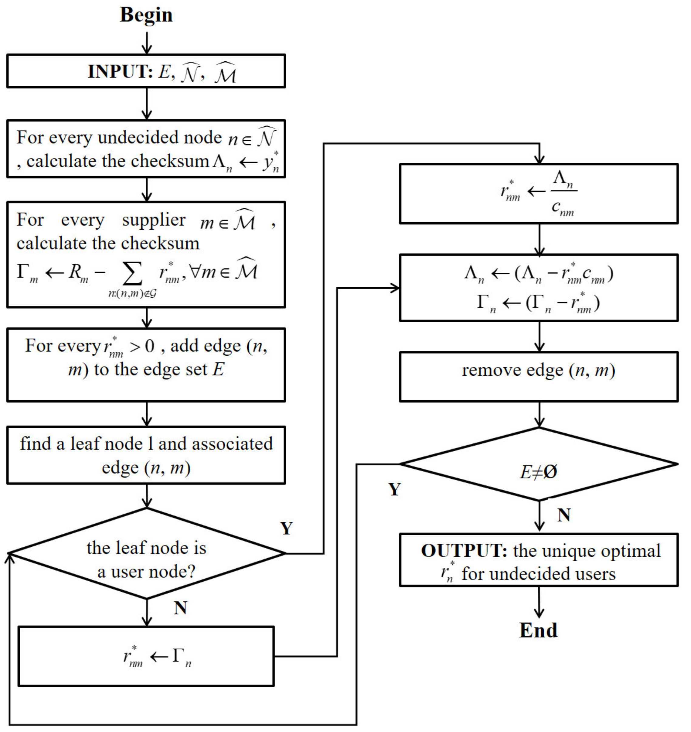
In this study, we explain the user-supplier interaction in the 5G wireless system using a two-stage extended game with comprehensive information (see [27]). To understand how to apply our model in a practical 5G wireless system, we take a 5G popular technology as a specific example. Then we explain how the two-stage works. Suppliers set their commodity pricing in the first stage, and consumers select the amount and supplier in the second stage. A user may choose the less costly commodity with poor service or the more expensive commodity with superior service. Based on users’ responses to suppliers’ prices, the suppliers take advantage and maximize profits. With this in mind, we first create a prototype that provides consumers with a variety of services and distinct outputs for providers. A multistage game model is utilized to describe the user-supplier relationship, and the user and supplier quantities are independently distributed. Next, we consider a social welfare maximization situation and determine that there must be an optimal solution. At that point, we move to the supplier competition game, which generates a decentralized algorithm that gradually finds equilibrium. The flowchart of the proposed algorithm is shown in Figure 1. Users make decisions based merely on the suppliers’ set price; meanwhile, suppliers determine the pricing based on demand (the user’s want). Finally, we present numerical results that demonstrate the efficacy of the suggested approach.

Our model aims to address the lack of a strong strategy to address the mismatch between supply and demand in the current 5G market, as well as the insufficient structure of market, which can have extremely negative effects. The model provides the user with a perspective on how to select a supplier, also provides a perspective for suppliers on the needs of users. It targets welfare maximization and provides an efficient way of managing supply and demand-side constraints. At the same time, the model helps to motivate market participants to make decisions that are most beneficial to the remaining economic agents.

2. The Model

Let us start with the features of 5G. In this section, 5G wireless networks will surpass the mobile Internet. In addition to increasing data rates compared to today’s 4G and 4.5G (LTE Advanced), new IoT and key communication examples will require new ways to improve performance. For example, “low latency” is about providing real-time interactivity for services that use the cloud: this is crucial to the success of self-driving cars for example. In addition, low power consumption enables networked objects to run for months or years without human assistance.

To better understand our research, we explain some notions here. As we set about formulating our problem, initially, we assume there are two sets: $\mathcal{M}=\{1,\dots ,M\}$ represent the 5G wireless suppliers and $\mathcal{N}=\{1,\dots ,N\}$ represent the 5G wireless users. Supplier $m\in \mathcal{M}$ provides a $R_m$ unit commodity to the users to maximize its return. User $n\in \mathcal{N}$ buys commodities from one or more suppliers to maximize its payoff. We assume that each user utilizes orthogonal resources, there is no interference between them, and meanwhile, the communication can be upward or backward. We simplify the interaction to be a multileader-follower game (see [28,29]), with suppliers leading the way and users following. In a relatively static network environment, channel gains are almost constant and also, public information is known to both sides. For example, every supplier gathers its respective channel information on every user and then applies it to all users. Section 4 assumes that our decentralized algorithm yields the same outcome as the supplier competition game.

2.1. Supplier Competition Game

There are two stages in the supplier competition game. Each supplier claims its price in the first stage. In the price vector b = [$b_1$,…,$b_M$], $b_m$ represents the price for the unit commodity that supplier m charges. In addition, every user $n\in \mathcal{N}$ chooses a demand from different suppliers, depicted by vector $r_n$ = [$r_{n1}$,…,$r_{nM}$]. Then we use a vector to depict the overall demand: r = [$r_1$,…,$r_N$].

In the second stage, as prices b have already been set, user n selects its demand $r_n$ to maximize its payoff based on the price. We define the payoff as a utility after subtracting expenses:

$$v_n(r_n,b)=u_n(\sum _{m=1}^M{r}_{nm}{c}_{nm})-\sum _{m=1}^M{b}_m{r}_{nm}.$$

(1)

In this equation, $c_{nm}$ is the offset of channel quality between provider m and user n (see Example 1 and Assumption 2). Here, $u_n$ is the utility function, which is concave and increases with quantity. We can see that the utility function is based on the term ${\sum }_{m=1}^M{r}_{nm}{c}_{nm}$, which is the amount of service that users acquire, and also the function of commodity uses. In the first stage, after taking into account the resource constraint ${\sum }_{n=1}^N{r}_{nm}⩽R_m$, and in the second stage, after factoring users’ demand, then supplier m sets the price to $b_m$ to maximize its return $b_m{\sum }_{n=1}^N{r}_{nm}$. We assume linear pricing, with each user facing the same price.

In this model, any user can buy a commodity from more than one supplier simultaneously. In other words, for users, n, more than one $r_{nm}$ ($m\in M$) can be positive. It may be reasonable only if the user’s device has several wireless interfaces. Interestingly, for most users ($N-M$ at least), the optimal strategy is to select one or no supplier.

In the following, a specific example shows how to apply our model in a practical 5G wireless system.

Example 1

(NOMA). Non-Orthogonal Multiple Access (NOMA) is a popular technology to improve the efficiency of the 5G spectrum, with low latency, low signaling cost, and attenuation resistance (see [30,31]). $W_m$, $m\in \mathcal{M}$ are the non-orthogonal frequency bands on which wireless providers operate. $r_{nm}$ is the portion of time user n can transmit exclusively on supplier m’s frequency band, in which ${\sum }_{n\in N_m}{r}_{nm}=1$, $m\in \mathcal{M}$ is the constraint. We assume a peak power constraint $P_n$ exists as well for each user. Then we define $c_{nm}$ as $W_{m}log(1+\frac{P_n{\left|h_{nm}\right|}^2}{{\sigma }_{nm}^2{W}_m})$ by Shannon’s theorem, in which the channel’s Gaussian noise variance is ${\sigma }_{nm}^2$ between provider m and user n, while $h_{nm}$ is channel gain, channel gain describes the transmission capability characteristics of the channel itself. The payoff for the user, then, is the remaining utility after subtracting payment for the service, $v_n=u_n({\sum }_{m=1}^M{r}_{nm}{c}_{nm})-{\sum }_{m=1}^M{b}_m{r}_{nm}$.

Similarly, our model applies when suppliers sell bandwidth of ultra-reliable low latency communication (uRLLC) tones to users who face a maximum power constraint [32]. For example, $c_{nm}$—the offset factor in Example 1—not only represents channel capability but essentially any aspect of the channel capacity’s increasing function. Compared with other previous technologies, 5G has a more significant channel gain. According to the Shannon formula, when the channel gain $h_{nm}$ increases, the channel capacity $c_{nm}$ will increase to achieve an extremely low delay.

Although the payment for the 5G service is high, the significant improvement of quality of service(QoS): utility function $u_n$, is enough to offset the payment, and the final income is significantly higher than that of time division multiple access(TDMA), and it can also meet the requirements of low delay and high spectrum efficiency in modern times.

Finally, we find that this problem resembles a generalized network flow setting’s multipath routing problem. A user parallels a source, similar to how a supplier corresponds to a link. Fortunately, there is one fundamental similarity: the multipath routing problem is equal-weighted, which applies to our model and does not hold in the TDMA model.

2.2. Assumptions about the Model

To focus on the problem of social welfare optimization, we make hypotheses, ignoring some unnecessary factors in the supplier competition game. Here, we outline our model assumptions.

Assumption 1.

$u_n\left(y\right)$ is increasing, differentiable, and strictly concave in y for each user $n\in \mathcal{N}$. In the network literature, this is how resilient data applications typically are modeled.

Assumption 2.

We draw offset $c_{nm}$ for the channel’s quality from continuous, different probability distributions. $c_{nm}$ are independent of each other, and evidently, different $c_{nm}$ cannot be equal. $c_{nm}$ indicates that a user will have different results if it buys the same commodity quantity from different suppliers.

As Example 1 shows, $c_{nm}$ is a function of $h_{nm}$, which is the channel gain between a supplier and user. Given that $h_{nm}$ is drawn from the independent continuous-probability distributions, these assumptions can be fulfilled. In the next section, we study a related socially optimal resource-allocation problem to analyze the supplier competition game. Additionally, we show the solution based on a user’s unique demand. In Section 4, we return to the supplier competition game. We find that the socially optimal, unique solution resembles the supplier competition game’s unique equilibrium. Here, even when suppliers and users are selfish, the game remains as efficient as previously.

3. Social Welfare Optimization

3.1. Maximizing Social Welfare

In the following, we study social welfare, a problem where we maximize the sum of payoffs for both users and suppliers. We show that the solution is unique based on the user’s demand. As users pay for advanced 5G resources and give money to suppliers, the payments between users and suppliers offset one another. Therefore, to maximize social welfare, we need to maximize users’ utility functions. We define the social welfare maximization problem as a function of service acquired by users, which is ultimately inherent to users’ interests.

Definition 1.

Let $y=[y_1,\dots ,y_N]$ be the vector of services acquired, where the service acquired by user n, $y_n={\sum }_{m=1}^M{r}_{nm}{c}_{nm}$ acts as a function of $r_n=[r_{n1},\dots ,r_{nM}]$, the demand for resources by user n.

Then we define the social welfare optimization problem (SWO) as

$$\begin{array}{cc}\hfill SWO:& maxu\left(y\right)=\sum _{n=1}^N{u}_n\left(y_n\right)+c\hfill \\ \hfill s.t.& \sum _{n=1}^N{r}_{nm}=R_m,m\in \mathcal{M}\hfill \\ \hfill & \sum _{m=1}^M{r}_{nm}{c}_{nm}=y_n,n\in \mathcal{N}\hfill \\ \hfill over& r_{nm},y_n\ge 0,\forall n\in \mathcal{N},m\in \mathcal{M}.\hfill \end{array}$$

(2)

Here, c is a variable that denotes the unpredictable change, but for simplicity, we set c = 0. Two variables comprise the SWO: the service-acquired vector y and the demand vector r. In fact, y is uniquely determined by r. So y is a function of variable r. Then we can write y as $y\left(r\right)$. For brevity, we write $u\left(y\right(r\left)\right)$ as $u\left(r\right)$.

3.2. Socially Optimal Demand Vector $r^{*}$’s Uniqueness

However, it is interesting that $u_n(·)$s fail to be strictly concave to the demand vector $r_n$, as is the case of SWO to r. As we all know, a maximization problem that is not strictly concave may have more than one global optimal solution (see [33,34]). To get more than one solution of vector $r^{*}$ in SWO, we simply modify $c_{nm}$s, $R_m$s, and $u_n(·)$s to some value. For example, if $c_{nm}$ is constant and the same for different n, m as it is for $R_m$, we can get a non-unique maximizer of SWO. However, as we showed previously, $c_{nm}$s are independent random variables from continuous distributions, and the probability of that case occurring is zero (see Assumption 2).

As we also learn in Lemma 1, no two maximizing demand vectors can exist in SWO that possess the same nonzero components. If two maximizing demand vectors combine, the result is still a maximizing demand vector. Finally, with the previous intermediate result, we see that maximizing demand vectors yields no convex combinations possessing different nonzero components, and this contradicts Lemma 1. So, we can use this to prove the primary finding of this section (Theorem 1).

Next, we define a demand vector $r_n$’s support set.

Definition 2.

User n’s support set is composed of suppliers from which user n’s demand is strictly positive:

$${\widehat{\mathcal{M}}}_n\left(r_n\right)=\{m\in \mathcal{M}:r_{nm}>0.\}$$

Given demand vector r, we define the support sets’ ordered collection ${\widehat{\mathcal{M}}}_1,{\widehat{\mathcal{M}}}_1,\dots ,{\widehat{\mathcal{M}}}_N$ as ${\{{\widehat{\mathcal{M}}}_n\}}_{n=1}^N$.

Lemma 1.

If $r^{*}$ is SWO’s maximizing demand vector containing the corresponding collection of support sets of ${\{{\widehat{\mathcal{M}}}_n\}}_{n=1}^N$, then it is almost true that $r^{*}$ can be a unique maximizing demand vector compared to ${\left\{{\widehat{\mathcal{M}}}_n\right\}}_{n=1}^N$.

Proof. 

Equation (2) holds for the maximizing demand vector $r^{*}$, and $r^{*}$ is uniquely constructed from ${\left\{{\widehat{\mathcal{M}}}_n\right\}}_{n=1}^N$. □

Then two categories exist for the users: decided and undecided.

We define that the decided users are those who buy from one supplier $(|{\widehat{M}}_n|=1)$, while the undecided users are those who buy from more than one supplier $(|{\widehat{M}}_n|>1)$. In fact, some users will buy nothing. Without loss of generality, these users are defined as decided users. $y_n^{*}={\sum }_{m=n}^M{r}_{nm}^{*}{c}_{nm}$ holds for all users. If user n is a decided user—which means that he only buys from supplier m and buys nothing from other suppliers—we can reduce the equation to $y_n^{*}=r_{n\overline{m}}^{*}{c}_{n\overline{m}}$, because other terms are zero. Then the unique demand vector that corresponds is $r_n^{*}=[0\dots 0,\frac{y_n^{*}}{c_{n\overline{m}}},0\dots 0]$.

Theorem 1.

There is a unique maximizing solution $b^{*}$ with probability 1 in SWO. There are no multiple maximizing demand vectors, and the convex combination of SWO for maximizing demand vectors retains the same support.

Proof. 

Suppose that more than one SWO optimal demand vector exists. Two of them are $r^{\prime }$ and $r^{*}$. We learn from Lemma 1 that $r^{*}$ and $r^{\prime }$ almost certainly have distinct support sets ${\left\{{\widehat{M}}_n^{*}\right\}}_{n=1}^N$ and ${\left\{{\widehat{M}}_n^{\prime }\right\}}_{n=1}^N$. Then, let $r^{\lambda }=\lambda r^{*}+\overline{\lambda }{r}^{\prime },\lambda \in \left(0,1\right),\overline{\lambda }=1-\lambda$. If $y_n^{*}={\sum }_{m=1}^M{r}_{nm}^{*}{c}_{nm}={\sum }_{m=1}^M{r}_{nm}^{\prime }{c}_{nm}$ and ${\sum }_{m=1}^M{r}_{nm}^{\lambda }{c}_{nm}=\lambda {\sum }_{m=1}^M{r}_{nm}^{*}{c}_{nm}+\overline{\lambda }{\sum }_{m=1}^M{r}_{nm}^{\prime }{c}_{nm}=y_n^{*}$, then we can say that $r^{\lambda }$ is an SWO maximizing solution for each $\lambda \in (0,1)$. Next, we can say that support set ${\widehat{M}}_n^{\lambda }\left(r^{\lambda }\right)=\left\{m\in \mathcal{M}:r_{nm}^{\lambda }=\lambda r_{nm}^{*}+\overline{\lambda }{r}_{nm}^{\prime }>0\right\}$ when user n is ${\widehat{M}}_n^{\lambda }={\widehat{M}}_n^{*}\cup {\widehat{M}}_n^{\prime }$, for every $\left(\lambda \in (0,1)\right)$. Note that the support sets $\left({\left\{{\widehat{M}}_n^{\lambda }\right\}}_{n=1}^N\right)$, in particular, are the same for all $\left(\lambda \in (0,1)\right)$. If two maximizing demand vectors exist with different support sets of SWO, then the convex combinations of SWO for two maximizing demand vectors retain the same support. This contradicts Lemma 1. □

We prove the uniqueness and existence of a Lagrange multiplier vector $b^{*}$ based on an SWO’s optimal demand vector $r^{*}$ [35]. In the following, we explain how the supplier competition game’s unique equilibrium is ($r^{*}$, $b^{*}$).

4. Game Analysis

So far, with the multileader-follower supplier competition game, we showed that the equilibrium is existing and unique, which is compared to the Lagrange multipliers and SWO’s unique optimal solution. Now, here we explain that the Lagrange multipliers are prices announced by suppliers. Furthermore, in this equilibrium, there are no more than $M-1$ undecided users.

The equilibrium concept is interpreted as follows [27]:

Definition 3.

Say that we have a subgame perfect equilibrium (SPE) with a price demand tuple $(b^{*},r^{*})$, in which no participant would like to change at any stage of the game. Moreover, given the price $b^{*}$, every user maximizes their payoff. Given users’ demand, $r^{*}\left(b^{*}\right)$ and other participants’ price, every supplier maximizes its return.

The equilibrium is solved by backward induction. In Stage 2, the users’ equilibrium strategy, users choose the best amount of resource $r^{*}\left(b\right)$ based on the vector of prices b. The function of Stage 2 is used to substitute the terms in Stage 1, the suppliers’ equilibrium strategy, resulting in equilibrium price $b^{*}$. According to BGR decoding, $r^{*}\left(b\right)$ is uniquely determined by equilibrium price $b^{*}$.

4.1. Users’ Equilibrium Strategy

Taking every user’s decision into account, we can solve the problem of user payoff maximization (UPM):

$$UPM:\underset{r_n⩾0}{max}{v}_n=\underset{r_n⩾0}{max}{u}_n(\sum _{m=1}^M{r}_{nm}{c}_{nm})-\sum _{m=1}^M{b}_m{r}_{nm}.$$

(3)

Lemma 2.

Regarding the UPM problem, with each maximizer $r_n$, ${\sum }_{m=1}{c}_{nm}{r}_{nm}=y_n^{*}$, for a unique nonnegative value of $y_n^{*}$. Furthermore, for any m such that $r_{nm}>0$, $\frac{b_m}{c_{nm}}={min}_{k\in M}\frac{b_k}{c_{ik}}$.

Proof. 

We can easily verify that Slater’s conditions are satisfied via UPM [36]. The following are the Karush–Kuhn–Tucker (KKT) conditions required for an optimal solution $r_n\ge 0$ of UPM of user n:

$$u_n^{\prime }\left(y_n\right)c_{nm}\le b_m,m\in \mathcal{M}$$

(4)

$$r_{nm}(u_n^{\prime }\left(y_n\right)c_{nm}-b_m)=0,m\in \mathcal{M},$$

(5)

$$where{y}_n=\sum _{m=1}^M{r}_{nm}{c}_{nm},r_n\ge 0.$$

(6)

Here, (4) implies that $u_n^{\prime }\left(y_n\right)\le \phi$, where $\phi ={min}_{k\in \mathcal{M}}\frac{b_k}{c_{nk}}.$ Based on user n’s utility function, two scenarios are possible: $u_n^{\prime }\left(0\right)<\phi$ and $u_n^{\prime }\left(0\right)\ge \phi$.

For the first scenario, $u_n^{\prime }\left(0\right)c_{nm}-b_m<0$, so $c_{nm}{u}_n^{\prime }\left(y_n\right)-b_m<0$ for all $m\in \mathcal{M}$ since, by Assumption 1, $u_n^{\prime }(·)$ is a marginal utility-with a strictly decreasing function. So, keeping (5) in mind, $r_{nm}=0$ for all $m\in \mathcal{M}$. Then $r_n=0$, and with (6), we see $y_n^{*}=0$. So, Equations (4)–(6) hold for the $y_n^{*}=0$ unique value.

With the second scenario, $u_n^{\prime }\left(0\right)\ge \phi$. However, keeping in mind that $u_n^{\prime }(·)$ dwindles to zero (Assumption 1), a unique ${\widehat{y}}_n\ge 0$ exists, such that $u_n^{\prime }\left({\widehat{y}}_n\right)=\phi$. First, we make sure $r_n$ exists, such that Equations (4)–(6) hold with $y_n={\widehat{y}}_n$. We find that Equation (4) holds, because $u_n^{\prime }\left({\widehat{y}}_n\right)=\phi \le b_m/c_{nm}$ for all $m\in \mathcal{M}.$ Then, with (5), we remember that for any m such that $b_m/c_{nm}>\phi =u_n^{\prime }\left({\widehat{y}}_n\right)$ there is $r_{nm}=0$. For any other m, $b_m/c_{nm}=\phi =u_n^{\prime }\left({\widehat{y}}_n\right)$, so, when it comes to (5), $r_{nm}$ can take any non-negative value. In particular, so that (6) holds for the set $\left\{m\in \mathcal{M}:b_m/c_{nm}=\phi \right\}$, it is possible to choose $r_{nm}$’s.

We provide the last part of the lemma by noting that $r_{nm}$ is positive only when $b_m/c_{nm}=\phi$. It remains to be seen whether ${\widehat{y}}_n$ is the only value of $y_n$ for which $r_n$ satisfies Equations (4)–(6). We can say that for any $y_n<{\widehat{y}}_n$, $u_n^{\prime }\left(y_n\right)>\phi$, which violates (4) for $m\in argmin{b}_k/c_{nk}$. Then, for each $y_n>{\widehat{y}}_n,u_n\left(y_n\right)<\phi$, which means that $u_n\left(y_n\right)c_{nm}-b_m<0$ for every $m\in \mathcal{M}$. Equation (5) implies, then, that $r_{nm}=0$ for every $m\in \mathcal{M}$, meaning that $y_n=0$; this is contradictory to $y_n>{\widehat{y}}_n>0$. The unique searched value $y_n^{*}$ is thus ${\widehat{y}}_n$. □

Definition 4.

Each supplier $m\in \mathcal{M}$ with $\frac{b_m}{c_{nm}}={min}_{k\in \mathcal{M}}\frac{b_k}{c_{ik}}$ is included in user n’s preference set ${\mathcal{M}}_n\left(b\right)$ for price vector b.

According to Lemma 2 and Section 2, we can divide users into decided and undecided users based on the preference sets’ cardinality. The support sets in Section 2 are quite similar to the preference sets. However, unlike support sets where users buy resources from suppliers, it is just possible for a user to request a resource from suppliers in the preference set. Evidently, the support set acts as a subset for the preference set: ${\widehat{\mathcal{M}}}_n\left(r\left(b\right)\right)\subset {\mathcal{M}}_n\left(b\right)$. Knowing this, we set about using the preference sets to construct a BGR so that there are on-loops with probability 1.

We define the Lagrange multipliers $b^{*}$ as prices. Every user knows this information, so it is not difficult to calculate the preference sets of other users and construct the BGR in comparison. Undecided users can determine their unique demand vector using a BGR decoding algorithm. For this, we consider all the demand vectors at a specific time and consider the equality of supply and demand. Then we find the uniqueness of the demand from BGR decoding. Although an infinite amount of best responses exist under prices $b^{*}$, the supply and demand will balance only if the demands are found by BGR decoding. Later, we prove that it is the supplier competition’s unique SPE.

4.2. Suppliers’ Equilibrium Strategy

The user’s utility functions determine the suppliers’ optimal choice of prices. A utility function $u_n$ can be characterized by its coefficient of relative risk aversion [37], i.e., $k_{RRA}^n=-\frac{{yu}_n^{″}\left(y\right)}{u_n^{\prime }\left(y\right)}$. This quantity characterizes the relationship between price and user demand.

Assumption 3.

Relative risk-aversion coefficient. $k_{RRA}^n<1,\forall n\in N$.

Some utility functions satisfy Assumption 3—for example, $log(1+y)$ and the $\phi -fair$ utility function s $\frac{y^{1-\phi }}{1-\phi }$, for $\phi \in (0,1)$[38]. To maximize the return, a monopoly will sell all the resources $R_m$. Once a supplier decreases the price, the users’ demand substantially increases, resulting in the supplier earning more than before. Thus, the supplier will lower the price until total supply and total demand are equal.

Theorem 2.

In keeping with Assumption 3, SPE as a price vector tuple meeting KKT conditions. We constitute the supplier competition game’s SPE using the Lagrange multiplier vector $b^{*}$ and SWO’s unique socially optimal demand vector $r^{*}$.

Proof. 

Suppose $b=[b_1,b_2,\dots ,b_M]$ is the price that suppliers charge. As defined in Equation (3), every user faces a local maximization problem UPM${}_n\left(b\right)$. Given Assumption 3, we further remark that r is an SPE of the supplier competition game only if each supplier’s supply equals demand, n.e., ${\sum }_{n=1}^N{r}_{nm}=R_m$ for every $m\in \mathcal{M}$. So, we consider the SPE as a price vector tuple meeting KKT conditions. Moreover, these meet the KKT conditions for any vector tuple b, r to be the SWO’s maximizing solution. We, therefore, designed a formal equivalence between the maximizing demand vector and SPE of the supplier competition game and the SWO problem ($r^{*},b^{*}$)’s Lagrangian multipliers. From this, we deduce that ($r^{*},b^{*}$) form the supplier competition game’s unique SPE. □

That social efficiency is not reduced by suppliers’ competition results in users’ utility functions being strictly concave and the users’ demand is relatively elastic. Therefore, if the price decreases a bit; demand will increase so much that the return is more than before. If suppliers set the price different from the optimal price $b^{*}$, the supply and demand are unequal. According to Theorem 2, we define the supplier competition game’s unique SPE $(b^{*},r^{*})$ as the equilibrium.

5. The Algorithm

Here, we provide a continuous-time algorithm, in which all the variables are functions of time. For brevity, we write $r_{nm}\left(t\right)$ and $b_m\left(t\right)$ as $r_{nm}$ and $b_m$, respectively. Then we write their time derivatives $\frac{\partial r_{nm}}{\partial t}$ and $\frac{\partial b_m}{\partial t}$ as $\dot{r_{nm}}$ and $\dot{b_m}$. Note that $r^{*}$ is the SWO’s unique maximizer, while the corresponding Lagrange multiplier vector is $b^{*}$. According to Theorem 2, we know that the supplier competition game’s unique SPE is $(b^{*},r^{*})$, and its values are invariant.

Given the demand vector $r_n\left(t\right)$, we write user N’s marginal utility according to $r_{nm}$ as ${\psi }_{nm}\left(t\right)$ or simply ${\psi }_{nm}$.

$${\psi }_{nm}=\frac{\partial u_n\left(r_n\right)}{\partial r_{nm}}=c_{nm}\frac{\partial u_n\left(y\right)}{\partial y}{|}_{y=y_n={\sum }_{m=1}^M{r}_{nm}{c}_{nm}}.$$

(7)

Here, we denote ${\psi }_{nm}\left(t\right)$’s value evaluated at $r_n^{*}$ as ${\psi }_{nm}^{*}$. Then we define column vectors: $\nabla u_n\left(r_n\right)={[{\psi }_{n1},\dots ,{\psi }_{nM}]}^T$ and $\nabla u_n\left(r_n^{*}\right)={[{\psi }_{n1}^{*},\dots ,{\psi }_{nM}^{*}]}^T$.

Next, ${\left(y\right)}^{+}=max(0,y)$ is defined, so that

$${\left(y\right)}_x^{+}=\left\{\begin{array}{cc}y& \begin{array}{c}x>0\end{array}\\ {\left(y\right)}^{+}& \begin{array}{c}x\le 0.\end{array}\end{array}\right.$$

In the following, the standard primal-dual variable update algorithm is motivated by the work in [25]:

$${\dot{r}}_{nm}=k_{nm}^r{({\psi }_{nm}-b_m)}_{r_{nm}}^{+},n\in \mathcal{N},m\in \mathcal{M}$$

(8)

$${\dot{b}}_m=k_m^b{(\sum _{n=1}^N{r}_{nm}-R_m)}_{b_m}^{+},m\in \mathcal{M}.$$

(9)

Here, $k_{nm}^r$ and $k_m^b$ are the constants that represent update rates. It is ensured that a variable of interest ($r_{nm}$ or $b_m$) will not turn negative when it is zero, even if the update’s direction is negative. We define the tuple $\left(r\right(t),b(t\left)\right)$ controlled by Equations (8) and (9) as the differential equations’ solution trajectory. Users only need to be given the prices that suppliers request. The providers do not need to be given other suppliers’ demands of the users, except for that of their resources. Only user n needs to know $c_{nm},m\in \mathcal{M}$.

The procedure of bipartite graph representation is as follows. First of all, for every undecided node $n\in \widehat{\mathcal{N}}$, calculate the checksum ${\Lambda }_n\leftarrow y_n^{*}$. Then, for every supplier $m\in \widehat{\mathcal{M}}$ calculate the checksum ${\Gamma }_m\leftarrow R_m-{\sum }_{n:(n,m)\notin \mathcal{G}}{r}_{nm}^{*}$, $\forall m\in \widehat{\mathcal{M}}$. Next, for every $r_{nm}^{*}>0$, add edge $(n,m)$ to the edge set E. And we have two steps in the loop. Step 1, Find a leaf node l and associated edge $(n,m)$, if the leaf node is a user node, then $r_{nm}^{*}\leftarrow \frac{{\Lambda }_n}{c_{nm}}$, else $r_{nm}^{*}\leftarrow {\Gamma }_n$. Step 2, Let ${\Lambda }_n\leftarrow ({\Lambda }_n-r_{nm}^{*}{c}_{nm})$ and ${\Gamma }_n\leftarrow ({\Gamma }_n-r_{nm}^{*})$, remove edge $(n,m)$. Keep doing these two steps until $E\in \varnothing$.

To find the unique optimal $r_n^{*}$ for undecided users, the algorithm provides detailed procedures. Here, E, $($, and $($ are sets of edges, user nodes, and supplier nodes separately. Using the algorithm, we can find the demand of undecided users. Because the probability that a BGR has no loops is 1, suppose that the BGR is an unrooted tree. Then an uncomplicated iterative algorithm can remove a node with a single associated edge, which we define as a leaf node and its incoming edge at each iteration. First, a leaf node is found in the BGR. Second, the demand of the leaf node’s incoming line is given from BGR Feature (1) or (2). Third, the parent node’s check-sum is updated with this value. Finally, the leaf node and incoming edge are removed. This process is one iteration. Iterate until no edges exist in the graph.

We can run the step finding the demand of undecided users because the probability that a BGR has no loops is 1, and we suppose that the BGR has no loops. However, in the last iteration, only one supplier node m plus one user node n exist, connected via an edge with value $r_{nm}^{*}$. ${\Lambda }_n$ and ${\Gamma }_m$ are their check-sums, which satisfy ${\Lambda }_n={\Gamma }_m{c}_{nm}$, because ${\Lambda }_n=r_{nm}^{*}{c}_{nm}$ and ${\Gamma }_m=r_{nm}^{*}$. At last, undecided users’ unique demand is given by the algorithm.

6. Numerical Results

We need to expand the settings to get numerical results. In Example 1, the fraction of time restricted to the 5G wireless supplier’s frequency band is the resource that is being sold, i.e., $R_m=1$ for $m\in \mathcal{M}$. Let $W_m$ = 700 MHz, $m\in \mathcal{M}$. $W_m$ means the 5G wireless suppliers’ bandwidth. $a_n$ log(${\sum }_{m=1}^M{r}_{nm}{c}_{nm}+1$) is user n’s utility function, in which the spectral efficiency $c_{nm}$ from the Shannon formula $\frac{1}{2}Wlog(1+\frac{E_b/N_0}{W}{\left|h_{nm}\right|}^2)$, $a_n$ is the “willingness to pay” factor, which we assume is the same among users, $r_{nm}$ is allocated time fraction, and $E_b/N_0$ is the transmit power divided by thermal noise.

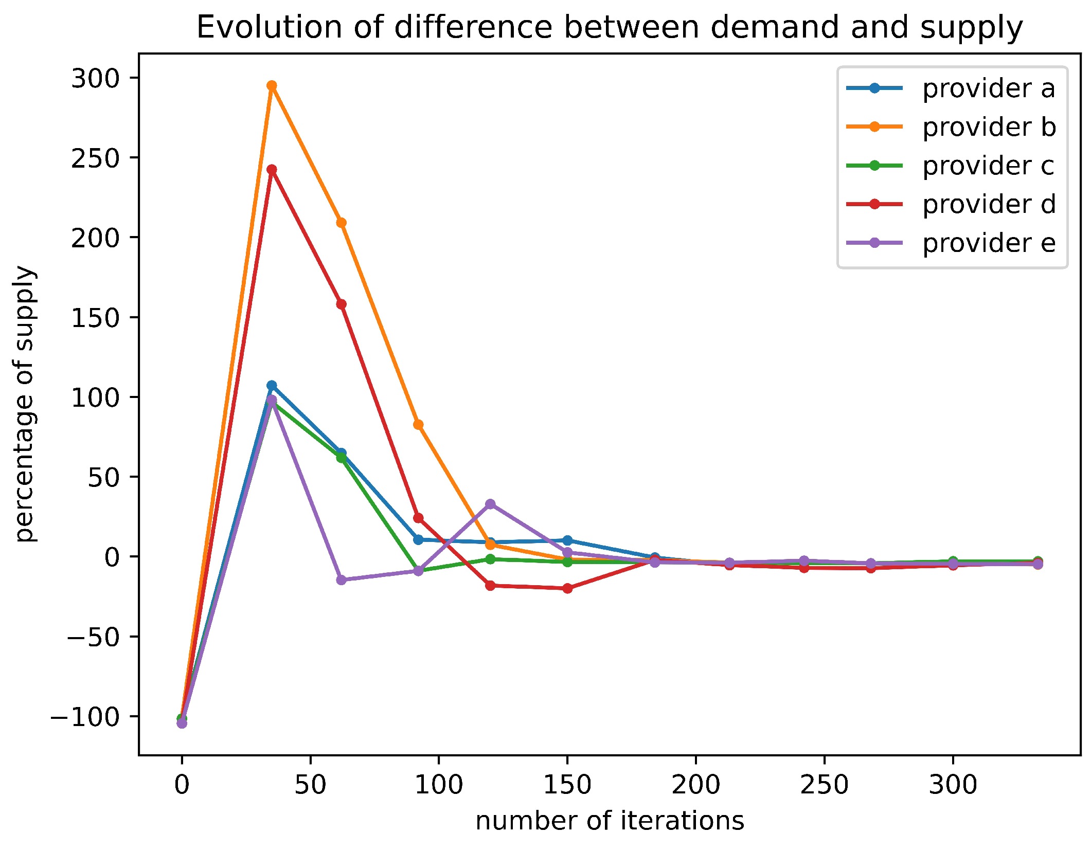
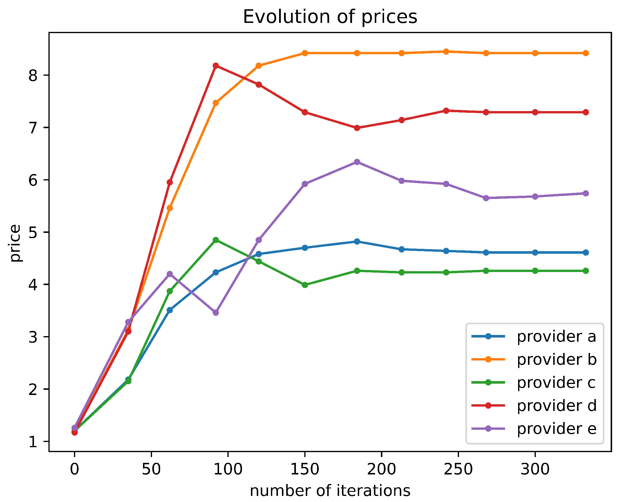
Suppose that the coding choices and modulation are perfect, with a continuum of values supplying a steady communication rate. Users are placed, then, uniformly in field that is $500\times 500$ square meters. We only provide these parameters to elucidate our point; we can change the numbers and the theory still applies to the parameters. Let us think of an example in the 5G background with 5 suppliers and 20 users. In Figure 2 and Figure 3, the equilibrium prices are represented as dashed lines. The competition among users can influence the equilibrium. Notice that supplier d offers a higher price than supplier a. Therefore, although supplier d can provide better resource quality, the user’s choice will also be affected by the equilibrium prices. Meanwhile, supplier b has the most buyers, its price is the highest, as Figure 2 and Figure 3 shows.

As for the convergence time in the discrete-time version: Suppose there are only five suppliers, then the number of users increases from 20 to 100. At each condition, we repeat the experiments 2000 times with random locations of suppliers and users. That way, we can obtain the average convergence speed and plot it. We define convergence as the number of iterations after which $\epsilon R_m$ is larger than the gap between demand and supply. For different $\epsilon$,

Table 1. Average time to convergence for different $\epsilon$. When $\epsilon R_m$ is larger than the gap between demand and supply, we define the number of iterations as convergence. In comparison, the smaller the parameter $\epsilon$, the larger the gap between supply and demand, so more iterations are required. For instance, if $\epsilon ={10}^{-3}$, the time to convergence is 2000–4000 in most cases, if $\epsilon ={10}^{-7}$, the time to convergence is 6000–12,000.

	Number of Users	$\mathit{\epsilon }={10}^{-3}$	$\mathit{\epsilon }={10}^{-4}$	$\mathit{\epsilon }={10}^{-5}$	$\mathit{\epsilon }={10}^{-6}$	$\mathit{\epsilon }={10}^{-7}$
	20	2022.4	3105.7	4209.9	5314.0	6209.9
	30	2068.8	3006.3	4068.8	5110.5	6110.5
	40	2407.0	3802.9	5011.2	6302.9	7532.0
	50	2786.8	4203.5	5807.7	7016.0	8203.5
Number of iterations	60	3145.8	4833.3	6312.5	8020.8	9520.8
	70	3525.6	5129.8	7025.6	8733.9	10,067.3
	80	3988.8	5509.6	7530.4	9509.6	10,926.3
	90	4243.6	6035.3	8056.1	10,076.9	11,931.1
	100	4435.9	6456.8	8435.9	10,540.1	12,519.3

shows the average convergence time. Generally, if $\epsilon ={10}^{-3}$, the time to convergence is 2000–4000. If $\epsilon ={10}^{-4}$, the time to convergence is 3000–6000.

In

Table 2. Average time to convergence for different numbers of suppliers when $\epsilon ={10}^{-3}$. The chart shows that when the ratio of suppliers to users is too high or low, the algorithm will iterate many times to converge. For instance, nearly 7000 iterations are required for 9 suppliers and 20 users. When the number of users increases gradually, the number of users is approximately positively correlated with the average convergence time.

	Number of Users	5 Suppliers	7 Suppliers	9 Suppliers
	20	6814.7	4199.3	3199.3
	30	3947.5	3493.0	3045.4
	40	3493.0	3793.7	3793.7
Number of iterations	50	3849.6	4150.3	4255.2
	60	4402.0	4604.8	4807.6
	70	4807.6	5101.3	5304.1
	80	5108.3	5437.0	5611.8
	90	5611.8	5723.7	6108.3
	100	6059.4	6213.2	6562.9

, we change the number of suppliers and see how the average convergence time changes. Now, let $\epsilon ={10}^{-4}$, and let it be constant. The update rates decide the convergence time: with low rates, the variables are likely to stabilize, and they will not take long to converge. In contrast, with high rates, the variables may converge rapidly. Based on Section 4’s theoretical analysis, to obtain the algorithm’s global convergence, let us distribute update variables randomly. Generally, the algorithm will iterate many times to converge if the ratio of users per supplier is too low or too large.

At last,

Table 3. Including standard deviation in the average time to convergence.

	Number of Users	Mean	Standard Deviation
	20	3098.0	2397.7
	30	3053.3	899.1
	40	3804.0	1095.1
Number of iterations	50	4208.9	853.1
	60	4798.3	1002.9
	70	5306.9	904.9
	80	5608.1	1089.3
	90	6013.0	1037.5
	100	6510.1	1198.8

presents the average convergence time when there are five suppliers with the standard variation. If the number of users is not 20, it does not affect the convergence time variance. If the number of users per supplier is under 4, update rates significantly impact the algorithm. In Table 2, we find that demands and prices vibrate and converge slowly in such instances.

7. Conclusions

This paper considers the competition between a random number of 5G wireless providers to attract users with different channel gains and willingness to pay. In this study, we utilized a two-stage wireless provider game to simulate the interaction in this work, and we proved the convergence and unique equilibrium. In the provider competition, our findings show that there is only one socially optimum resource allocation. At equilibrium, there are some undecided users. There are also fewer undecided users than providers. Finally, we designed a decentralized algorithm that uses only regional information to converge to the equilibrium demand vectors and price.