Article

A Graph-Cut-Based Approach to Community Detection in Networks

1
School of Electronic and Electrical Engineering, Hongik University, Seoul 04066, Korea
2
Department of Civil and Environmental Engineering, Hongik University, Seoul 04066, Korea
*
Author to whom correspondence should be addressed.
Appl. Sci. 2022, 12(12), 6218; https://doi.org/10.3390/app12126218
Submission received: 6 May 2022 / Revised: 14 June 2022 / Accepted: 16 June 2022 / Published: 18 June 2022
(This article belongs to the Special Issue Artificial Intelligence in Complex Networks)

Abstract

:
Networks can be used to model various aspects of our lives as well as relations among many real-world entities and objects. To detect a community structure in a network can enhance our understanding of the characteristics, properties, and inner workings of the network. Therefore, there has been significant research on detecting and evaluating community structures in networks. Many fields, including social sciences, biology, engineering, computer science, and applied mathematics, have developed various methods for analyzing and detecting community structures in networks. In this paper, a new community detection algorithm, which repeats the process of dividing a community into two smaller communities by finding a minimum cut, is proposed. The proposed algorithm is applied to some example network data and shows fairly good community detection results with comparable modularity Q values.

1. Introduction

Graphs consisting of vertices and edges can be used to model various aspects of our lives and real-world environments. For example, social media services can model each service subscriber as a vertex and a friend relationship between two individuals as an edge connecting the two corresponding vertices. Another example would be a water supply network; a pipe network connecting many water sources and consumers can be modeled as a graph. The Internet and the world wide web can be modeled as networks as well.
As networks can represent many abstract contexts of our lives, it is a natural desire to try to discover a core structure inherent in them. Partitioning a network via grouping vertices of similar affiliations can help us to grasp the main structure of a given network with a holistic viewpoint. In other words, a community structure of a network can give us a better understanding of its characteristics, properties, and inner workings. An example of community detection of a network is shown in Figure 1.
There has been significant research on detecting and evaluating community structures in networks. Many fields, including social sciences, biology, engineering, computer science, and applied mathematics, have identified their own needs for developing methods to analyze and detect community structures in networks. Graph partitioning problems in graph theory are also closely related to the community detection problem. Many algorithms for community detection and clustering have been proposed so far, and there are a few extensive review papers on them [1,2].
The main contribution of this paper is to propose a new community detection algorithm, which repeats the process of dividing a community into two smaller communities by finding a minimum cut of the community. In order to compute the minimum cut of a community, the betweenness centrality values of vertices are used to choose the source and sink nodes. The modularity criterion is used in a greedy way to determine the local optimal partition among many candidate communities to be cut.
The rest of this paper is organized as follows. Section 2 briefly reviews prior work on community detection methods. Section 3 presents the proposed algorithm, and Section 4 illustrates the results of the algorithm applied to a few example networks. Finally, Section 5 discusses the results and concludes the paper.

2. Prior Works

Uncovering community structures inherent in networks can shed light on many aspects of our world because networks can model various relations and inner workings among entities and objects. Therefore, community detection in networks has received a lot of attention from many fields [2,3,4,5,6,7], and it is rapidly evolving. Scientists and researchers from various fields have accordingly produced a large number of research articles and study results.
The community detection problem has been studied mainly for static networks, but the problem has also been studied for dynamic networks as well as overlapping communities recently [8,9,10,11,12,13,14]. At their initial development phase, community detection algorithms concerned disjoint communities, where each vertex of a network belongs to only one community. However, many real-world networks such as social networks can have overlapping communities, so that a vertex is permitted to belong to several communities at the same time. Even though the problems for dynamic networks or overlapping communities are interesting and worth tackling, this paper limits its scope to methods for disjoint community detection of static networks.
Since it is unrealistic to review all the previously proposed algorithms for community detection, only a few representative algorithms are mentioned in this section. More detailed reviews and studies regarding community detection can be accessed through several extensive review articles and books [2,3,4,5,15,16,17].
Even though many algorithms for community detection have been proposed so far, it seems that there is no single algorithm that can detect communities universally well for many kinds of various networks [18,19]. Therefore, it is believed to be better to have multiple different algorithms and apply suitable one to each particular network. Most algorithms proposed for disjoint community detection of static networks may be classified into three categories: traditional, modularity-based, and dynamic algorithms [2].
Traditional algorithms include hierarchical clustering [1,20,21,22,23,24], Girvan–Newman (GN) algorithms [25,26,27,28] and their variants [29,30,31], spectral clustering [32,33,34,35,36,37,38,39], and graph-partitioning-based algorithms [39,40]. Most of these algorithms are based on clustering, and they have provided basic concepts of community detection for later developments.
Modularity-based algorithms include the Guimera and Amaral algorithm [41], the fast GN algorithm [27], the Clauset algorithm [42], optimization-based algorithms [25,41,43,44,45,46], and genetic algorithms [47,48,49,50,51]. The concept of modularity was introduced by Newman and Girvan [25], and modularity-based algorithms try to optimize the modularity value by finding a good community structure in a network via some heuristics. The concept of modularity is briefly reviewed in Section 3.
Dynamic algorithms include those that are based on spin models, random walk, and synchronization. A random walk can be used for community detection by letting an entity make random moves along the edges of a network [52,53,54,55]. More details on dynamic algorithms can be found in review papers and books [2,3,4,5].
Since many algorithms and methods for community detection have been proposed, the task of evaluating them becomes important as well. To measure the performance of the algorithms and methods, a few standard benchmarks of complex networks with known community structures have been devised. Among these benchmarks, the GN and LFR (Lancichinetti, Fortunato, and Radicchi) benchmarks are frequently used [56,57]. These benchmark networks are synthesized with predetermined community structures, and an algorithm is evaluated by comparing the result of community detection to the known answer, i.e., the predetermined community structure. Besides these synthetic benchmarks, there are some real-world network data that are frequently used to evaluate community detection algorithms. In Section 4, some of these real-world network data are used to illustrate the performance of the algorithm proposed in this paper.

3. Methods

The community detection method proposed in this paper is based on the idea that connections between vertices of the same community tend to be denser than connections between vertices of different communities. Since a minimum cut in graph theory finds as few connections to a cut as possible, applying a minimum cut to a network may give us boundaries between different communities. In other words, a minimum cut might result in a cut-set that contains more inter-connections between communities than intra-connections within communities.
The proposed method of this paper iteratively applies the minimum cut solution to a network to generate a community structure. The method first finds two temporary source and sink nodes that are expected to be of different communities, and computes a minimum cut between the two nodes. As a result of the cut, the network is divided into two groups. Then, the same procedure is applied to each group, and quality measures of the resulting community structures of the entire network are compared to select the better result between the two. The same procedure is repeated until no further refinement of the quality of community structure is obtained. A precise description of the proposed algorithm is presented later in this section.

3.1. Network and Community Structure

To describe the problem and the proposed algorithm precisely, some basic notations are introduced.
Definition 1.
A network is a graph G = ( V , E ) defined by V and E, where V and E are the set of vertices (nodes) and the set of edges, respectively. An edge is a pair of two vertices. Given a network G = ( V , E ) and a subset C V of vertices, E ( C ) E is a subset of E consisting of all the edges whose endpoints belong to C.
This paper concerns undirected graphs without loops or multiple edges even though the proposed method may be easily extended to the case of directed graphs. Therefore, an edge e = { u , v } E is a pair of two vertices u , v V , and the order of the two is not relevant unless it is noted otherwise. We also assume that the graph is connected; every pair of vertices ( u , v ) of G has a path from u to v. In this paper, networks are used interchangeably with graphs.
Definition 2.
A community structure C = { C 1 , C 2 , , C k } of a network G = ( V , E ) is a partition of V, the set of vertices of G. In other words, i = 1 k C i = V and C i C j = for i , j = 1 , , k with i j . Here, k refers to the number of communities of the community structure C.
With these definitions, the objective of the community detection problem can be stated as finding a good community structure C when a network G is given.

3.2. Minimum Cut

Since the minimum cut in graph theory is employed in the proposed method, a brief review is provided in this section.
Definition 3.
A cut C = ( S , T ) is a partition of the set of vertices V of a graph G = ( V , E ) into two subsets S and T. The cut-set of a cut C = ( S , T ) is the set { u , v } E | u S , v T of edges that have one endpoint in S and the other endpoint in T. If s and t are specified vertices of the graph G, then an s-t cut is a cut C = ( S , T ) such that s S and t T .
In this paper, we consider networks whose edges have no weight values assigned, i.e., unweighted and undirected graphs. However, graphs may have edge weights in general, and the weight of a cut in an undirected graph is defined as follows.
Definition 4.
In an unweighted and undirected graph, the size or weight of a cut is defined to be the number of edges that belong to the cut-set of the cut. In a weighted graph, the value or weight of a cut is defined to be the sum of the weights of the edges in the cut-set.
Given the definitions of a cut and the weight of a cut, a minimum cut of a network is defined as follows.
Definition 5.
A minimum cut of an undirected graph is a cut whose weight is not larger than the weight of any other cut.
It is well known in network science that the maximum flow of a flow network from a source vertex s to a sink vertex t is equal to the capacity of a minimum cut that separates the two vertices s and t. This result is called the max-flow min-cut theorem and was introduced by Ford and Fulkerson [58]. The Ford–Fulkerson method can be used to find a minimum cut and a maximum flow, and the Edmonds–Karp algorithm is an implementation of the method that runs in polynomial time [59,60].
Even though the max-flow min-cut theorem deals with a directed graph with capacity values assigned on edges, it is straightforward to extend the theorem to undirected and weighted graphs. Besides the Ford–Fulkerson method, there are other algorithms for finding a minimum cut of undirected edge-weighted graphs such as the Stoer–Wagner algorithm [61,62]. The Stoer–Wagner algorithm has the time complexity of O ( | V | | E | + | V | 2 log | V | )  [62].
Since the max-flow min-cut theorem is well known and there are many algorithms for finding a minimum cut of undirected graphs, we denote such an algorithm as MINIMUM-CUT without a detailed description of the procedure.
Definition 6.
Given a connected graph G = ( V , E ) , a capacity function c, and source and sink vertices s and t, the procedure MINIMUM-CUT ( G , c , s , t ) is an implementation of a method that finds a minimum cut of the graph G with c, s, and t.
The capacity function c in Definition 6 gives the weight value of each edge of a weighted graph, i.e., a capacity is used interchangeably with a weight in this paper. The MINIMUM-CUT procedure is employed in our proposed algorithm, and more details are described later.

3.3. The Betweenness Centrality

To apply MINIMUM-CUT to a graph, source and sink vertices s and t should be provided as well as the capacity c for each edge. For community detection, the source and sink vertices should be chosen so that the two vertices do not belong to the same community, because the two vertices are cut by MINIMUM-CUT. The betweenness centrality in graph theory is used to select two vertices in our proposed method. In particular, the two vertices of highest betweenness centrality values are chosen as the source and sink vertices in applying MINIMUM-CUT.
In graph theory, betweenness centrality is a measure of the centrality of a vertex in a graph [63]. Roughly speaking, the betweenness centrality of a vertex represents the degree of how many pairs of nodes are connected via the shortest paths passing through the vertex. The betweenness centrality c B ( v ) of a vertex v V of a graph G = ( V , E ) based on shortest paths is defined as the following
c B ( v ) = s , t V σ ( s , t | v ) σ ( s , t ) ,
where σ ( s , t ) is the number of shortest paths from s V to t V , and  σ ( s , t | v ) is the number of those paths passing through a vertex v other than s and t [64,65]. If  s = t , we let σ ( s , t ) = 1 , and if v { s , t } , we let σ ( s , t | v ) = 0 . On unweighted graphs, computing betweenness centrality takes O ( | V | | E | ) times using Brandes’ algorithm [64].
As briefly mentioned before, the betweenness centrality values for all the vertices are computed to select the source and sink vertices s and t, which are provided as inputs to MINIMUM-CUT. Those two vertices of the highest values are chosen because it is expected that many shortest paths connecting vertices of different communities pass through these two nodes.

3.4. The DIVIDE-INTO-TWO Algorithm

To find a community structure of a given network, the proposed algorithm of this paper iterates by dividing a group of vertices into two smaller groups until a stopping criterion is satisfied. Before the algorithm is described precisely, we present the procedure of dividing a group of vertices into two smaller groups in Algorithm 1, called DIVIDE-INTO-TWO.
Algorithm 1: The DIVIDE-INTO-TWO algorithm.
   Input: A connected graph G = ( V , E )
   Output:  C = { C 1 , C 2 } , a partition of G
1:
   procedure DIVIDE-INTO-TWO(G)
2:
         if  | V | 1  then
3:
           C { V }
4:
         else
5:
          Compute betweenness centrality c B ( v ) for all v V
6:
           s arg max v V c B ( v )
7:
           t arg max v V \ { s } c B ( v )
8:
           S v V | { s , v } E
9:
           T v V | { t , v } E
10:
        for all  { u , v } E  do
11:
            c u v 1
12:
        end for
13:
        for all  v S  do
14:
           if  v T { t }  then
15:
               c s v
16:
           end if
17:
        end for
18:
        for all  v T  do
19:
           if  v S { s }  then
20:
               c t v
21:
           end if
22:
        end for
23:
         C MINIMUM-CUT ( G , c , s , t )
24:
          end if
25:
  end procedure
After the source s and sink t are selected by the betweenness centrality computation, DIVIDE-INTO-TWO initializes the capacity values of all the edges of the network to be one. Then, it assigns infinity as the capacity to the edges that are connected to the source or sink vertices. This assignment is to prevent the edges connected to s or t from being cut by MINIMUM-CUT. The procedure forms a group of vertices S and T, where vertices of S and T are neighbors of the source and sink nodes, respectively. The capacity value of infinity makes the vertices of groups S or T strongly connected to themselves, which prevents the edges from being cut by MINIMUM-CUT. All the other edges remain with a capacity of one, as initialized.
When assigning infinity as a capacity value to edges, it should be avoided that the source s and sink t are connected by a path whose every edge has infinity as its capacity value. If there is any path connecting the source and sink vertices where all the edges of the path have infinity as capacity, then MINIMUM-CUT cannot find a cut set of finite minimum cut value. To carefully assign infinity as capacity, DIVIDE-INTO-TWO checks whether the other vertex belongs to S or T, as described precisely in Algorithm 1.
Computing the betweenness centralities via Brandes’ algorithm takes O ( | V | | E | ) time, while the MINIMUM-CUT procedure takes O ( | V | | E | + | V | 2 log | V | ) time when using the Stoer–Wagner algorithm. The Stoer–Wagner algorithm is one of the fast algorithms for finding a minimum cut from a graph. Considering these time complexities, the DIVIDE-INTO-TWO algorithm has the same time complexity as MINIMUM-CUT. Note that all the other executions of DIVIDE-INTO-TWO except for the two main procedures can be performed in linear time. For example, selecting the source and sink vertices and forming the two sets S and T can be done in linear time. Assigning capacity values to all the edges also takes linear time.

3.5. Modularity: A Quality Measure

In most practical cases, community detection algorithms are applied to a network whose community structure is not known ahead of time. Therefore, it is necessary to have a quality measure to evaluate a community structure derived by a community detection algorithm. In other words, we need a measure to answer the question of how well the found community structure represents the underlying connection characteristics of the network.
Even though a quality measure of community structure is needed, there exists one difficulty in defining such a measure. There is no pre-defined precise answer for the community structure of a given network; two people may have different opinions about the inherent community structure of the same network. It is hard to say that a community structure of a network is strictly better than another community structure of the same network. Examples that illustrate this difficulty are presented in Section 4.
Although it is difficult to find a well-defined and unified quality measure to evaluate a particular division of a given network, some measures have been proposed so far. One of the widely used measures is modularity [25]. The modularity measure is defined as follows.
Definition 7.
Given a network G = ( V , E ) with a community structure C = { C 1 , C 2 , , C k } , a  k × k symmetric matrix M is defined, where each element M i j for i , j = 1 , , k is the fraction of all edges that connect vertices in community i to vertices in community j. Then, the modularitymeasure Q of the community structure C of the network G is defined by
Q ( C ; G ) = Tr M M 2 ,
where X is the sum of the elements of the matrix X.
Note that the row sum m i = j M i j of the matrix M represents the fraction of edges that have at least one vertex in community i at its endpoints. If all the pre-existing edges are removed and new edges are randomly placed between vertices while preserving the row sums, the expected fraction of all the new edges that connect vertices in community i and vertices in community j equals m i · m j . Therefore, the difference between the pre-existing and the expected fraction, M i i m i 2 , may be used as an indication of how strongly the vertices in the community i are connected to each other. In other words, it can measure how densely the vertices in the community i are linked. By adding these differences for all the k communities, the modularity measure can be defined as
Q = i = 1 k M i i m i 2 ,
which is shown to be equal to the right side of Equation (2).
The maximum value that Q can have is Q = 1 , and this value indicates a network with a very strong community structure [25,66]. The modularity Q values for networks with strong community structure usually range from about 0.3 to 0.7 .
Our proposed algorithm computes the modularity value after each division of the given network via graph cuts, and it determines the next step based on the calculated Q values. In particular, the Q value is used as a stopping criterion to stop iterations of community division. Therefore, the Q values are critical for the algorithm.

3.6. The Proposed Algorithm

The proposed algorithm is a divisive one, so that a given network is divided into groups of vertices in a stepwise manner. The main idea of the algorithm is that a connected network may be partitioned into two subgroups by finding a minimum cut separating the two, which is expected to reveal a good community structure of the given network. After a division of each connected component of a network, the Q value for the resulting community structure is calculated. By comparing the resulting Q value for every connected component, the algorithm selects the best partition and creates two communities out of the selected component. The algorithm iterates this process until no further improvement in the modularity value is observed. The algorithm is named MCCD (Minimum Cut-based Community Detection) and is presented precisely in Algorithm 2.
Algorithm 2: The MCCD algorithm.
   Input: A connected graph G = ( V , E )
   Output:  C = { C 1 , , C k } , a community structure of G
1:
   procedure MCCD(G)
2:
          C { V }
3:
          Q 0
4:
         loop
5:
            if  | C | = | V |  then
6:
               break
7:
            end if
8:
            for  i 1 to | C |  do
9:
                { C i 1 , C i 2 } DIVIDE-INTO-TWO( C i , E ( C i ) )
10:
               Q i Q { C 1 , , C i 1 , C i 1 , C i 2 , C i + 1 , , C | C | } ; G
11:
           end for
12:
            m arg max i Q i
13:
           if  Q > Q m  then
14:
              break
15:
           end if
16:
            C { C 1 , , C m 1 , C m 1 , C m 2 , C m + 1 , , C | C | }
17:
            Q Q m
18:
       end loop
19:
  end procedure
Note that the locally optimal partition { C 1 , , C m 1 , C m 1 , C m 2 , C m + 1 , , C | C | } , where m   =   arg max i Q i , is selected at each iteration of the MCCD algorithm. The iteration repeats until a decrease in the modularity Q value is observed or each vertex has its own community, i.e., the entire network is partitioned into one-vertex communities. As illustrated in Section 4, however, the Q value starts decreasing after only a few iterations for many networks. In other words, many networks are expected to have a community structure consisting of not so many communities.
Even though the MCCD algorithm stops its iteration of dividing each community into two smaller communities when it detects decreasing Q values, it is also possible to continue the iteration until a desired number of communities are obtained, via a slight modification of the algorithm. This modified algorithm is precisely presented in Algorithm 3 and is called k-MCCD. The desired number of communities k, which is given as an input, is assumed to satisfy 1 k | V | . As presented in Algorithm 3, k-MCCD stops its iterations when the number of communities reaches the desired number k.
Algorithm 3: The k-MCCD algorithm.
   Input: A connected graph G = ( V , E ) and a desired number of communities k
   Output:  C = { C 1 , , C k } , a community structure of G
1:
   procedurek-MCCD(G, k)
2:
          C { V }
3:
          Q 0
4:
         loop
5:
            if  | C | = k  then
6:
               break
7:
            end if
8:
            for  i 1 to | C |  do
9:
                { C i 1 , C i 2 } DIVIDE-INTO-TWO( C i , E ( C i ) )
10:
               Q i Q { C 1 , , C i 1 , C i 1 , C i 2 , C i + 1 , , C | C | } ; G
11:
           end for
12:
            m arg max i Q i
13:
            C { C 1 , , C m 1 , C m 1 , C m 2 , C m + 1 , , C | C | }
14:
            Q Q m
15:
       end loop
16:
  end procedure
As mentioned previously, the procedure DIVIDE-INTO-TWO has the time complexity of O ( | V | | E | + | V | 2 log | V | ) . Therefore, when MCCD calls DIVIDE-INTO-TWO( C i , E ( C i ) ) for a community C i , it takes O ( | C i | | E ( C i ) | + | C i | 2 log | C i | ) time. MCCD calls DIVIDE-INTO-TWO for each community C i during one iteration, so the total computation time summed for every community can be given by
i = 1 | C | O ( | C i | | E ( C i ) | + | C i | 2 log | C i | ) .
The computation time of Equation (4) satisfies
i = 1 | C | O ( | C i | | E ( C i ) | + | C i | 2 log | C i | ) i = 1 | C | O ( | C i | | E | + | C i | 2 log | C i | ) O ( | V | | E | + | V | 2 log | V | ) ,
where the convexity of a function f ( x ) = y x + x 2 log x for sufficiently large x is used for the second inequality.
Besides DIVIDE-INTO-TWO, another procedure should be accounted for when considering the time complexity of MCCD, which is the computation of the modularity Q i for each community C i . Assuming that the change in Q is tracked during the iterations, it is known that the time complexity of modularity computation is bounded by O ( | V | + | E | ) [27]. Therefore, the modularity computation does not affect the time complexity of MCCD, because DIVIDE-INTO-TWO takes a longer time. Since MCCD iterates dividing a community into two smaller communities until the stopping criterion is satisfied, in the worst case where the iteration number is equal to | V | , the time complexity of MCCD is given by O ( | V | 2 | E | + | V | 3 log | V | ) , which is in polynomial time. However, many practical networks are believed to have a small number of communities, which is equal to the total number of iterations of MCCD. Therefore, the time complexity of MCCD may be bounded by O ( | V | | E | + | V | 2 log | V | ) in those cases.

4. Results

This section describes the results of application of the proposed MCCD algorithm to four different example networks. The first example deals with a very simple network whose community structure is obvious. This example checks the validity of the proposed algorithm; if the algorithm cannot detect the obvious community structure of the simple network, it is useless to consider it any further. After the simple validity check, three more examples are used to show the performance of the MCCD algorithm. These examples are frequently used in the literature on the study of networks, so they can provide an evaluation of the performance of the proposed algorithm.

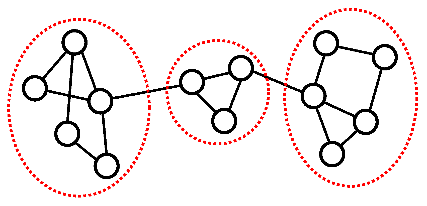
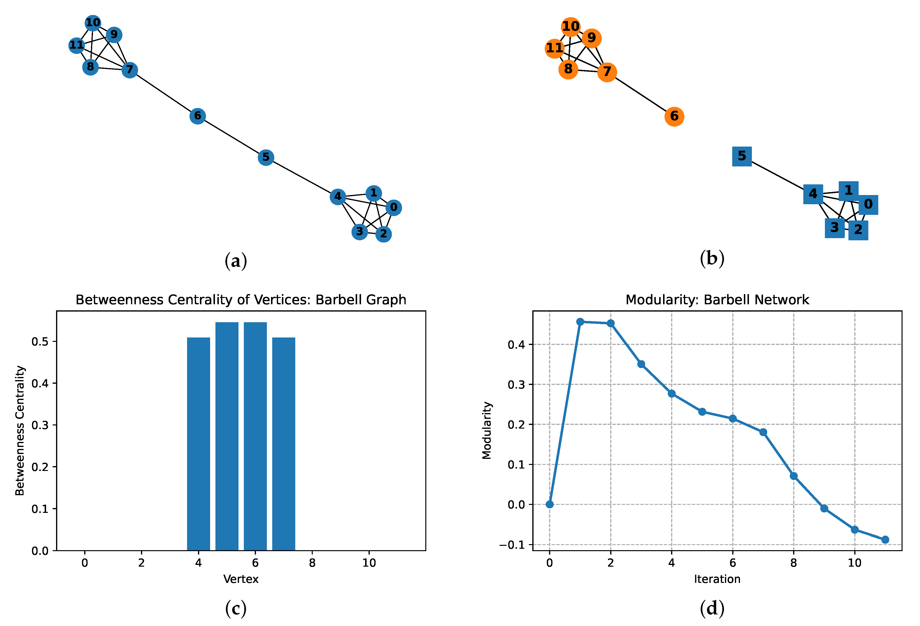
4.1. Example 1: A Simple Network

A very simple network, whose community structure is obvious, is generated as shown in Figure 2a. The network is a slightly generalized version of a graph, usually called an n-barbell graph, and it has two complete subgraphs that are connected by a path [67,68,69]. It is obvious that the network has two communities: C 1 = { 0 , 1 , 2 , 3 , 4 , 5 } and C 2 = { 6 , 7 , 8 , 9 , 10 , 11 } .
The result of the MCCD algorithm applied to the network is shown in Figure 2b. As expected, the MCCD algorithm detects the two obvious communities, and they are represented as blue rectangles ( C 1 ) and orange circles ( C 2 ) in the figure. Therefore, the MCCD algorithm works well for the simple barbell graph.
The betweenness centrality value c B ( v ) for all vertices v of the barbell network is shown in Figure 2c. Vertices 5 and 6, which are boundary nodes of each community, have the highest betweenness centrality value because the shortest paths connecting nodes of the network pass through them more than any other nodes. Therefore, the MCCD algorithm selects the two vertices 5 and 6 as the source and sink nodes at the first iteration of the process. The algorithm then succeeds in finding the minimum cut between the two vertices and in detecting the obvious communities C 1 and C 2 .
Note that the MCCD algorithm stops its iteration after the second pass because the modularity score of the second pass, which is about 0.4527 , is lower than that of the first pass, which is about 0.4565 . The modularity value of every iteration is shown in Figure 2d, where the MCCD algorithm is slightly modified to perform its iterations even though the modularity value Q m of each iteration starts decreasing; the lines 13–15 of MCCD Algorithm 2 are temporarily ignored to repeat the DIVIDE-INTO-TWO procedure until every edge is cut, so that each vertex forms its own community. As can be observed in Figure 2d, the modularity value quickly decreases as MCCD repeats its iteration passes.

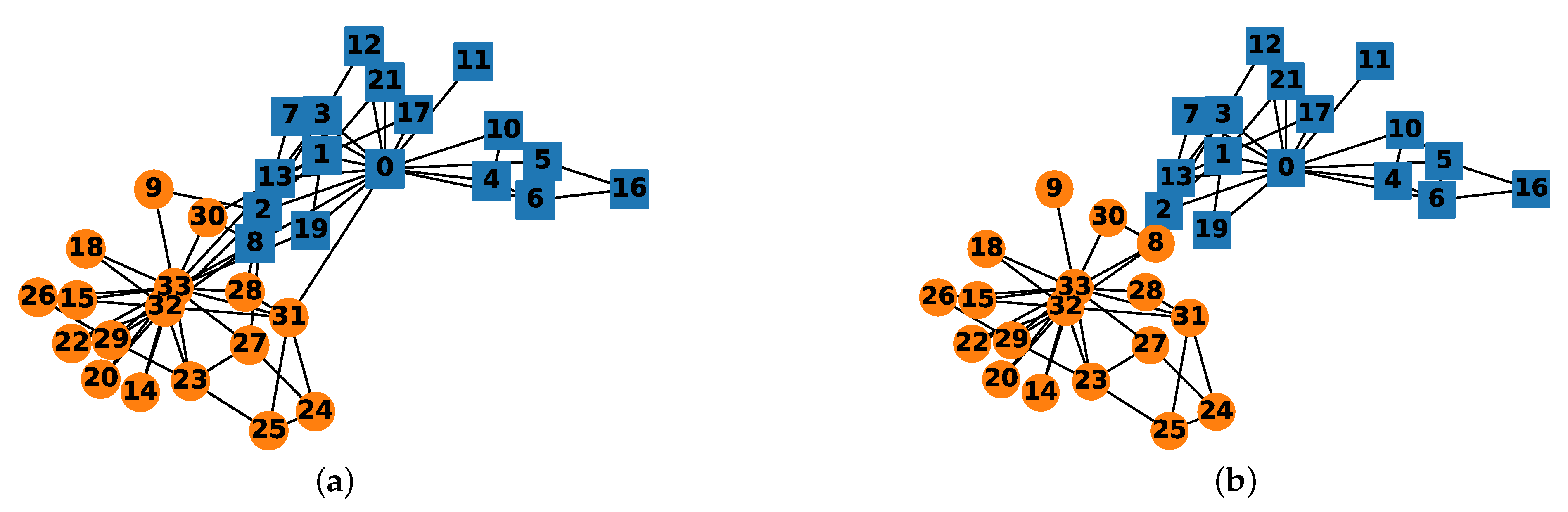
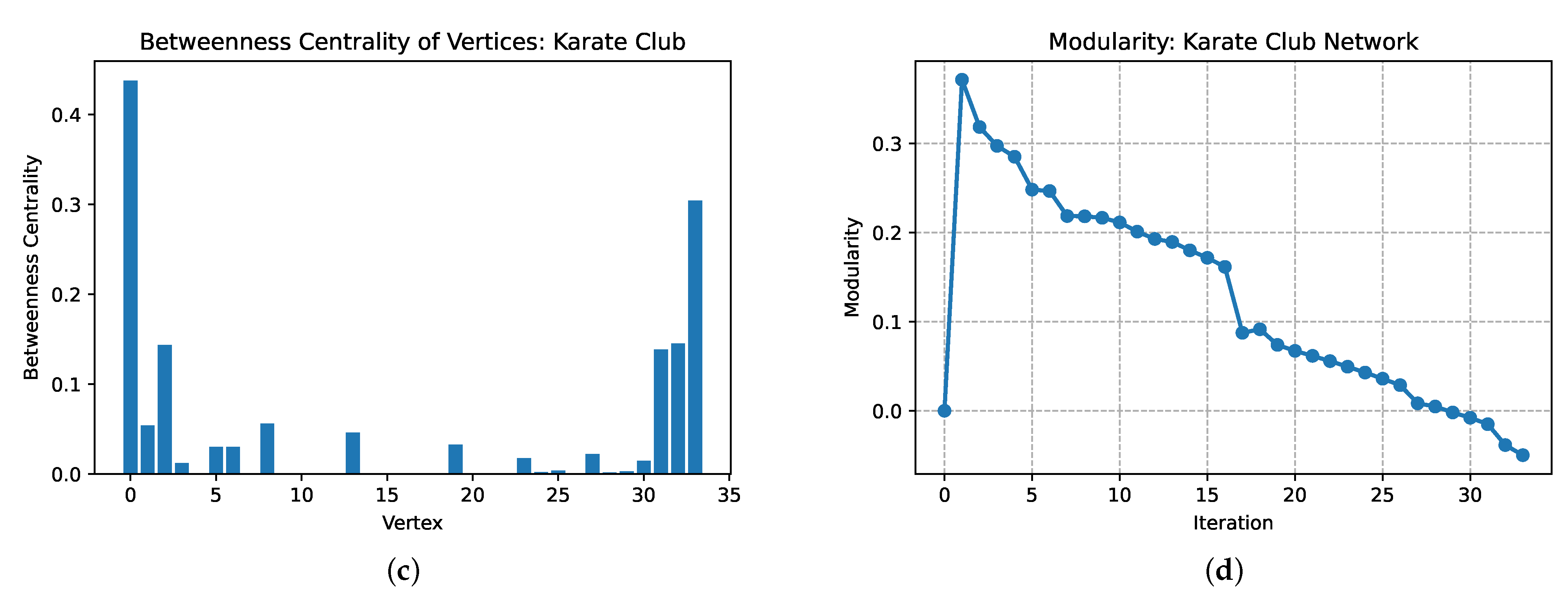
4.2. Example 2: Zachary’s Karate Club Network

One of the frequently used real-world network data is Zachary’s karate club network [7]. The karate club network represents social interactions between 34 individuals, who were the members of a karate club at a university. Wayne Zachary obtained the network data by observing social interactions between the members for a period of three years from 1970 to 1972.
Before the study began, the club had employed an instructor (Mr. Hi) for karate lessons. At the beginning of the study, there was a conflict between the instructor and the club president (John A.) over the price of karate lessons. The instructor wished to raise prices while the president wanted to stabilize them. As time passed, there arose a series of factional confrontations, and then the president fired the instructor for attempting to raise lesson prices unilaterally. The supporters of the instructor resigned and formed a new organization headed by the instructor, thus completing the fission of the club.
Figure 3a shows the karate club network, where each vertex represents a member of the club. Vertices 0 and 33 represent the instructor and the president, respectively; the members who belong to the group headed by the instructor after the fission are represented by blue square vertices and the members who belong to the other group are represented by orange circle vertices. An edge of the network is drawn if two individuals were observed to interact outside the normal activities of the club, i.e., if they could be said to be friends outside the club activities.
The result of the proposed MCCD algorithm is shown in Figure 3b. Comparing the result with the data shown in Figure 3a, only one vertex, which is labeled 8, is misclassified by MCCD; vertex 8 joined the organization headed by the instructor after the fission, but the MCCD algorithm predicts that it belongs to the other group. Therefore, it can be said that MCCD works well for the karate club network.
Figure 3c shows the betweenness centrality values c B ( v ) for the vertices of the network. As expected, the instructor and the president nodes have the highest values, so MCCD selects the two vertices as the source and sink nodes at its first iteration. The modularity values after each iteration of MCCD are shown in Figure 3d. The modularity value achieves its maximum value of 0.3715 after the first iteration, and the values quickly decrease as MCCD iterates its DIVIDE-INTO-TWO procedures.
To model information flow in the karate club, Zachary defined a capacitated network for the club, which includes a capacity matrix C whose entries are interpreted as representing a capacity or value of maximum possible information flow between two members of the club [7]. In other words, each edge of the network has a quantified value representing the strength/weakness of friend relationship between the two end vertices. These capacity values were assigned by analyzing data of social interactions between the club members. Using this capacitated network model, Zachary employed the max-flow min-cut theory and applied the labeling procedure of Ford and Fulkerson [58,70,71]. To apply the algorithm, the vertices 0 and 33 of the network were manually designated as the source and sink nodes.
Zachary obtained the same result as MCCD, which is expected, and explained why vertex 8 is misclassified [7]. One point to note is that, contrary to Zachary’s method, MCCD automatically selects the source and sink nodes and iterates the DIVIDE-INTO-TWO operation to find the best result for community detection.
Many community detection algorithms that have been proposed previously used the karate club network data to verify their performances, and the modularity results of a few well-known algorithms are shown in Table 1. Most algorithms result in higher modularity values than MCCD, but the ground truth of the karate club network has the modularity value of 0.371 [6]. As described above, MCCD misclassifies only one vertex, so that the modularity value of MCCD is very close to the ground truth. This result illustrates that modularity is not a perfect measure even though it is a very good one.
Table 1. Modularity values for the karate club network of a few well-known community detection algorithms and MCCD: Girvan and Newman (GN) [25]; Newman (FN) [27]; Clauset, Newman, and Moore (CNM) [42]; Duch and Arenas (DA) [72]. Data from [25,27,46,72].
AlgorithmGNFNCNMDAMCCD
Modularity0.4010.3810.3810.4190.372

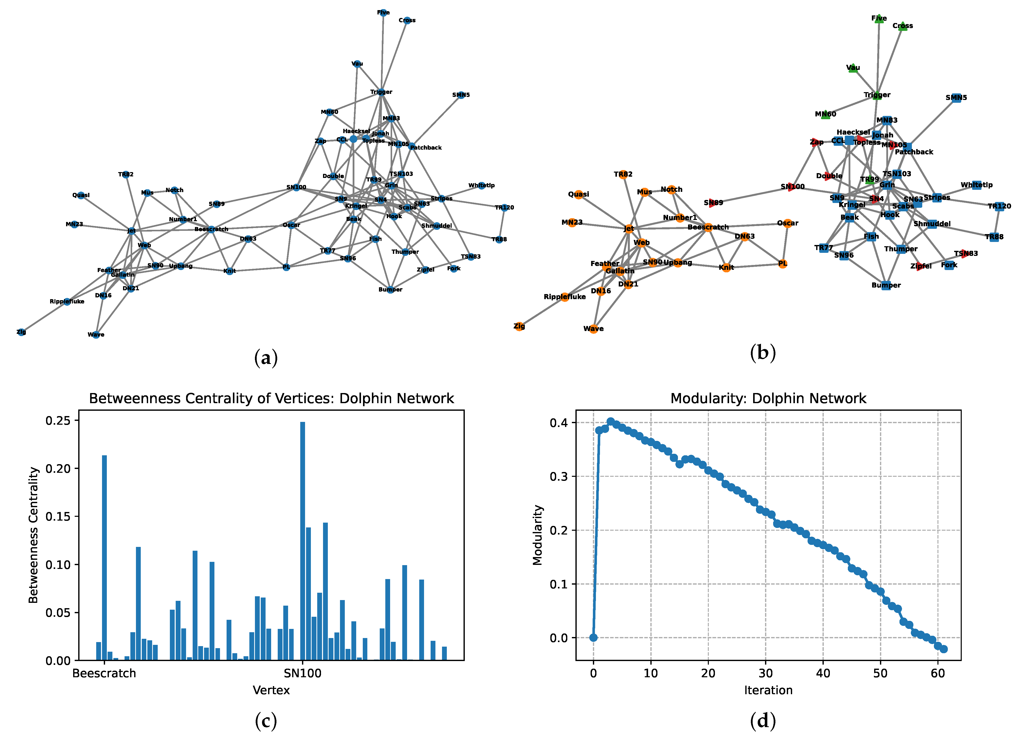
4.3. Example 3: The Social Network of Bottlenose Dolphins

The third example network is the social network of bottlenose dolphins that was studied by Lusseau [73]. Lusseau conducted a study about a social network of bottlenose dolphins residing in the Doubtful Sound, Fiordland, New Zealand, from November 1994 to November 2001. Based on the observations and study, 62 dolphins were formed into a social network, and it is shown in Figure 4a [74].
As can be seen from Figure 4a, the community structure of the dolphin network is not random, but it is not obvious, either. In other words, it seems that there is a weak community structure in the network, and different people may have different opinions on the structure as well as the number of communities. As mentioned before, it is hard to find a universally agreed answer for the community structure of a network, and this example illustrates this difficulty.
Figure 4b shows the result of MCCD application to the network. The modularity value achieved its maximum of 0.4021 after three iterations; hence, MCCD detects four communities shown in the figure. The betweenness centrality values of the vertices and the modularity values after each iteration are shown in Figure 4c,d, respectively. It turns out that the modularity values of the first few iterations are similar, and this implies that it is hard to tell which structure is best for community detection. Even though MCCD generates the four community structure, structures of slightly different numbers of communities are also plausible. Lusseau presented a sociogram with three groups in his original paper [74]. In fact, the whole network visually seems to have two large groups, where the network is divided into two groups mostly by the gender of dolphins: males and females.

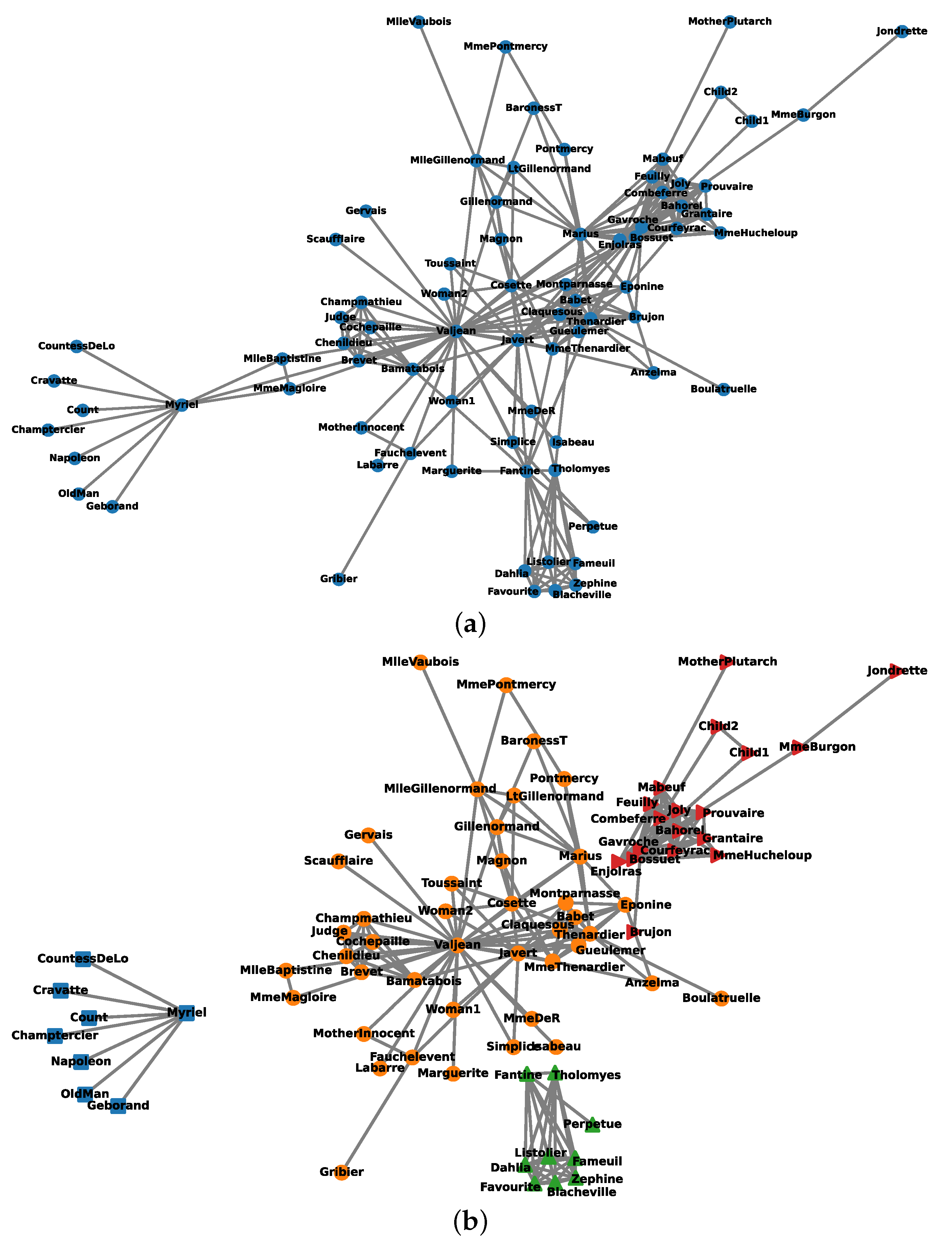
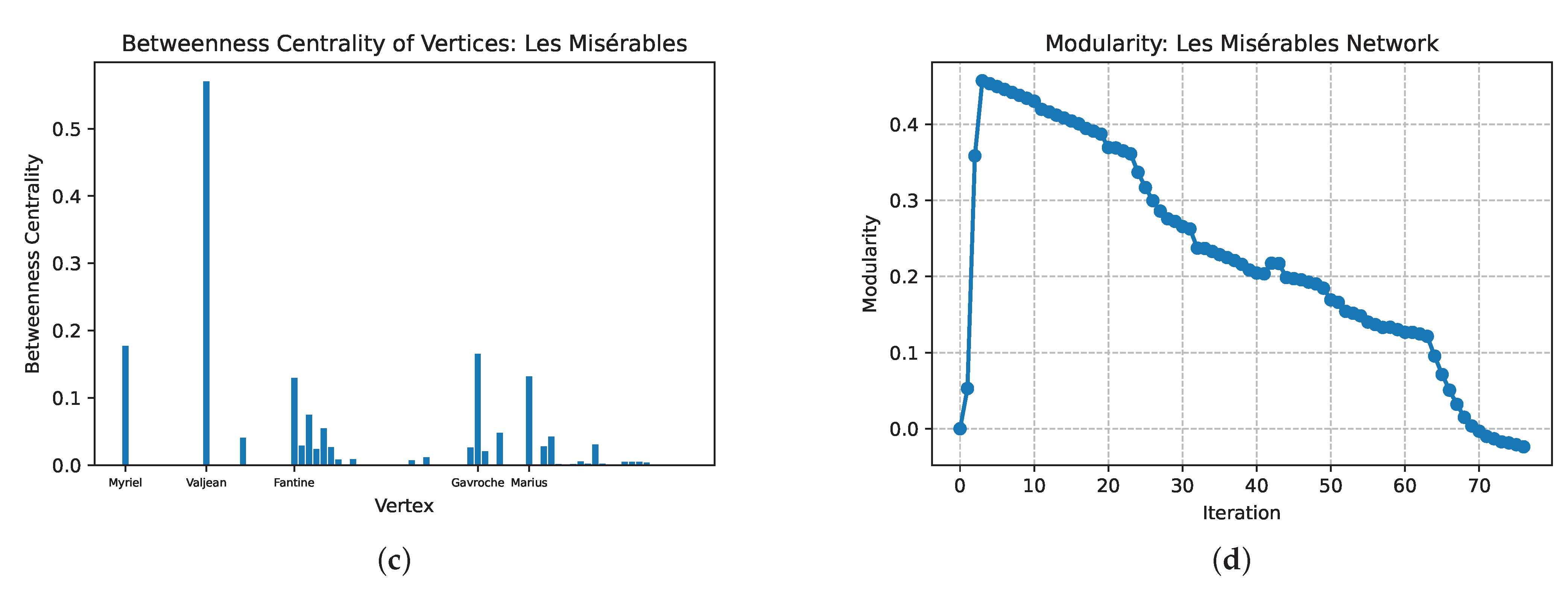
4.4. Example 4: The Characters Network of Les Misérables

Figure 5a shows the network of major characters in Les Misérables, a famous novel written by Victor Hugo. The network data was constructed by considering coappearances of characters in the same chapter of the book [75]. The 77 vertices of the network are major characters, and an edge between two vertices represents coappearance of the corresponding two characters in the same chapter. Even though Knuth assigned a value to each edge by counting the number of coappearances of the two characters, our method does not use the edge attribute values; MCCD uses the network structure only.
The result of MCCD application to the network is shown in Figure 5b. As shown in Figure 5d, the modularity value achieves its maximum of 0.4570 when the network is partitioned into four communities. As expected, the protagonist Jean Valjean and the police officer Javert form the central positions of the main community. Another community that consists mainly of the members of the Friend of the ABC, the fictional association of revolutionary French republican students, is also detected. Enjolras, the charismatic leader of the association, belongs to this community. Furthermore, two more communities are also detected, and it can be observed that these two are centered by the main characters Myriel and Fantine, respectively.

5. Discussion

In this paper, a new algorithm for community detection was proposed and some experimental results were provided. As previously mentioned, the problem of community detection has its inherent difficulties; there is no exact solution for the problem. People may have different opinions about the community structure of a given network. As seen in Section 4, the networks of bottlenose dolphins and of characters in the novel Les Misérables are complicated, so that there is no universally agreed-upon community structure. Even though the modularity measure Q can provide a criterion to estimate the quality of community structures, it is only an indirect measure, and some may find a lower-scored community structure to be better than a higher-scored one.
Considering that the problem of community detection has no exact solution, the proposed algorithm MCCD shows fairly good results with comparable Q values when applied to the example networks of Section 4. In particular, the algorithm shows satisfactory results for the barbell graph and Zachary’s karate club network. For the more complicated networks in Section 4, it also detects community structures well, which can be visually observed from Figure 4 and Figure 5.
Even though the proposed algorithm showed its feasibility via the example networks of Section 4, further evaluation of the performance of the algorithm by using various benchmarks and larger network data is needed and remains as future work. Frequently used benchmarks such as GN and LFR may be used for the evaluation. For the example networks of Section 4, MCCD takes a few seconds with typical current computers, but the time performance should be carefully investigated with larger networks and benchmarks.
Optimization of the MCCD algorithm implementation is also left as future work. Many procedures called by MCCD may be carefully modified and implemented to reduce computation time. Modifying the algorithm so that it can be applied to detect overlapping community structures may be left as another element of future work. This may not be easy, however, because graph cut methods in general divide vertices without overlapping.

Author Contributions

Conceptualization, H.S. and J.P.; methodology, H.S.; software, H.S.; validation, H.S., J.P. and D.K.; formal analysis, H.S.; investigation, J.P. and D.K.; resources, H.S. and D.K.; data curation, H.S.; writing—original draft preparation, H.S.; writing—review and editing, J.P. and D.K.; visualization, H.S.; supervision, H.S., J.P. and D.K.; project administration, D.K.; funding acquisition, H.S. All authors have read and agreed to the published version of the manuscript.

Funding

This research was supported partly by the Basic Science Research Program through the National Research Foundation of Korea (NRF) funded by the Ministry of Science and ICT (NRF-2019R1C1C1008017) and partly by the Hongik University new faculty research support fund.

Institutional Review Board Statement

Not applicable.

Informed Consent Statement

Not applicable.

Data Availability Statement

The data presented in this study are available in this article and there are no other data to share.

Conflicts of Interest

The authors declare no conflict of interest. The funders had no role in the design of the study; in the collection, analyses, or interpretation of data; in the writing of the manuscript, or in the decision to publish the results.

Abbreviations

The following abbreviations are used in this manuscript:
GNGirvan and Newman
LFRLancichinetti, Fortunato, and Radicchi
MCCDMinimum Cut-based Community Detection
CNMClauset, Newman, and Moore
DADuch and Arenas

References

  1. Fortunato, S. Community detection in graphs. Phys. Rep. 2010, 486, 75–174. [Google Scholar] [CrossRef] [Green Version]
  2. Javed, M.A.; Younis, M.S.; Latif, S.; Qadir, J.; Baig, A. Community detection in networks: A multidisciplinary review. J. Netw. Comput. Appl. 2018, 108, 87–111. [Google Scholar] [CrossRef]
  3. Danon, L.; Díaz-Guilera, A.; Duch, J.; Arenas, A. Comparing community structure identification. J. Stat. Mech. Theory Exp. 2005, 2005, P09008. [Google Scholar] [CrossRef]
  4. Lancichinetti, A.; Fortunato, S. Community detection algorithms: A comparative analysis. Phys. Rev. E 2009, 80, 056117. [Google Scholar] [CrossRef] [Green Version]
  5. Yang, B.; Liu, D.; Liu, J. Discovering Communities from Social Networks: Methodologies and Applications. In Handbook of Social Network Technologies and Applications; Furht, B., Ed.; Springer: Boston, MA, USA, 2010; pp. 331–346. [Google Scholar] [CrossRef]
  6. Cheng, J.; Leng, M.; Li, L.; Zhou, H.; Chen, X. Active Semi-Supervised Community Detection Based on Must-Link and Cannot-Link Constraints. PLoS ONE 2014, 9, e110088. [Google Scholar] [CrossRef]
  7. Zachary, W.W. An Information Flow Model for Conflict and Fission in Small Groups. J. Anthropol. Res. 1977, 33, 452–473. [Google Scholar] [CrossRef] [Green Version]
  8. Asur, S.; Parthasarathy, S.; Ucar, D. An Event-Based Framework for Characterizing the Evolutionary Behavior of Interaction Graphs. ACM Trans. Knowl. Discov. Data 2009, 3, 1–36. [Google Scholar] [CrossRef]
  9. Backstrom, L.; Huttenlocher, D.; Kleinberg, J.; Lan, X. Group Formation in Large Social Networks: Membership, Growth, and Evolution. In Proceedings of the 12th ACM SIGKDD International Conference on Knowledge Discovery and Data Mining, Philadelphia, PA, USA, 20–23 August 2006; pp. 44–54. [Google Scholar] [CrossRef]
  10. Dunlavy, D.M.; Kolda, T.G.; Acar, E. Temporal Link Prediction Using Matrix and Tensor Factorizations. ACM Trans. Knowl. Discov. Data 2011, 5, 1–27. [Google Scholar] [CrossRef] [Green Version]
  11. Fu, W.; Song, L.; Xing, E.P. Dynamic Mixed Membership Blockmodel for Evolving Networks. In Proceedings of the 26th Annual International Conference on Machine Learning, Montreal, QC, Canada, 14–18 June 2009; pp. 329–336. [Google Scholar] [CrossRef]
  12. Chakraborty, T.; Chakraborty, A. OverCite: Finding Overlapping Communities in Citation Network. In Proceedings of the 2013 IEEE/ACM International Conference on Advances in Social Networks Analysis and Mining, Niagara, ON, Canada, 25–28 August 2013; pp. 1124–1131. [Google Scholar] [CrossRef]
  13. Yang, J.; Leskovec, J. Overlapping Community Detection at Scale: A Nonnegative Matrix Factorization Approach. In Proceedings of the Sixth ACM International Conference on Web Search and Data Mining, Rome, Italy, 4–8 February 2013; pp. 587–596. [Google Scholar] [CrossRef]
  14. Maity, S.; Rath, S.K. Extended Clique percolation method to detect overlapping community structure. In Proceedings of the 2014 International Conference on Advances in Computing, Communications and Informatics (ICACCI), Delhi, India, 24–27 September 2014; pp. 31–37. [Google Scholar] [CrossRef]
  15. Gulbahce, N.; Lehmann, S. The art of community detection. BioEssays 2008, 30, 934–938. [Google Scholar] [CrossRef] [Green Version]
  16. Papadopoulos, S.; Kompatsiaris, Y.; Vakali, A.; Spyridonos, P. Community detection in Social Media: Performance and application considerations. Data Min. Knowl. Discov. 2012, 24, 515–554. [Google Scholar] [CrossRef]
  17. Chintalapudi, S.R.; Prasad, M.H.M.K. A survey on community detection algorithms in large scale real world networks. In Proceedings of the 2015 2nd International Conference on Computing for Sustainable Global Development (INDIACom), New Delhi, India, 11–13 March 2015; pp. 1323–1327. [Google Scholar]
  18. Plantié, M.; Crampes, M. Survey on Social Community Detection. In Social Media Retrieval; Ramzan, N., van Zwol, R., Lee, J.S., Clüver, K., Hua, X.S., Eds.; Springer: London, UK, 2013; pp. 65–85. [Google Scholar] [CrossRef] [Green Version]
  19. Yang, Z.; Algesheimer, R.; Tessone, C. A Comparative Analysis of Community Detection Algorithms on Artificial Networks. Sci. Rep. 2016, 6, 30750. [Google Scholar] [CrossRef] [PubMed] [Green Version]
  20. Wu, Z.; Leahy, R. An optimal graph theoretic approach to data clustering: Theory and its application to image segmentation. IEEE Trans. Pattern Anal. Mach. Intell. 1993, 15, 1101–1113. [Google Scholar] [CrossRef] [Green Version]
  21. Shen, H.; Cheng, X.; Cai, K.; Hu, M.B. Detect overlapping and hierarchical community structure in networks. Phys. A Stat. Mech. Its Appl. 2009, 388, 1706–1712. [Google Scholar] [CrossRef] [Green Version]
  22. Ahn, Y.Y.; Bagrow, J.P.; Lehmann, S. Link communities reveal multiscale complexity in networks. Nature 2010, 466, 761–764. [Google Scholar] [CrossRef] [Green Version]
  23. Barabási, A.L.; Albert, R. Emergence of Scaling in Random Networks. Science 1999, 286, 509–512. [Google Scholar] [CrossRef] [Green Version]
  24. Hastie, T.; Friedman, J.; Tibshirani, R. The Elements of Statistical Learning; Springer: New York, NY, USA, 2009. [Google Scholar] [CrossRef]
  25. Newman, M.E.J.; Girvan, M. Finding and evaluating community structure in networks. Phys. Rev. E 2004, 69, 026113. [Google Scholar] [CrossRef] [Green Version]
  26. Newman, M.E.J. Properties of highly clustered networks. Phys. Rev. E 2003, 68, 026121. [Google Scholar] [CrossRef] [Green Version]
  27. Newman, M.E.J. Fast algorithm for detecting community structure in networks. Phys. Rev. E 2004, 69, 066133. [Google Scholar] [CrossRef] [Green Version]
  28. Newman, M.E.J. Analysis of weighted networks. Phys. Rev. E 2004, 70, 056131. [Google Scholar] [CrossRef] [Green Version]
  29. Tyler, J.R.; Wilkinson, D.M.; Huberman, B.A. E-Mail as Spectroscopy: Automated Discovery of Community Structure within Organizations. Inf. Soc. 2005, 21, 143–153. [Google Scholar] [CrossRef] [Green Version]
  30. Wilkinson, D.M.; Huberman, B.A. A method for finding communities of related genes. Proc. Natl. Acad. Sci. USA 2004, 101, 5241–5248. [Google Scholar] [CrossRef] [PubMed] [Green Version]
  31. Rattigan, M.J.; Maier, M.; Jensen, D. Graph Clustering with Network Structure Indices. In Proceedings of the 24th International Conference on Machine Learning, Corvalis, OR, USA, 20–24 June 2007; pp. 783–790. [Google Scholar] [CrossRef]
  32. Shi, J.; Malik, J. Normalized cuts and image segmentation. IEEE Trans. Pattern Anal. Mach. Intell. 2000, 22, 888–905. [Google Scholar]
  33. von Luxburg, U. A tutorial on spectral clustering. Stat. Comput. 2007, 17, 395–416. [Google Scholar] [CrossRef]
  34. Donath, W.E.; Hoffman, A.J. Lower Bounds for the Partitioning of Graphs. IBM J. Res. Dev. 1973, 17, 420–425. [Google Scholar] [CrossRef]
  35. Fiedler, M. Algebraic connectivity of graphs. Czechoslov. Math. J. 1973, 23, 298–305. [Google Scholar] [CrossRef]
  36. Barnard, S.T.; Pothen, A.; Simon, H. A spectral algorithm for envelope reduction of sparse matrices. Numer. Linear Algebra Appl. 1995, 2, 317–334. [Google Scholar] [CrossRef] [Green Version]
  37. Meilă, M.; Shi, J. A random walks view of spectral segmentation. In Proceedings of the 8th International Workshop on Artificial Intelligence and Statistics, Key West, FL, USA, 4–7 January 2001; pp. 203–208. [Google Scholar]
  38. Ng, A.; Jordan, M.; Weiss, Y. On Spectral Clustering: Analysis and an algorithm. In Proceedings of the Advances in Neural Information Processing Systems, Vancouver, BC, Canada, 3–8 December 2001; Volume 14. [Google Scholar]
  39. Pothen, A. Graph Partitioning Algorithms with Applications to Scientific Computing. In Parallel Numerical Algorithms; Keyes, D.E., Sameh, A., Venkatakrishnan, V., Eds.; Springer: Dordrecht, The Netherlands, 1997; pp. 323–368. [Google Scholar] [CrossRef]
  40. Kernighan, B.W.; Lin, S. An Efficient Heuristic Procedure for Partitioning Graphs. Bell Syst. Tech. J. 1970, 49, 291–307. [Google Scholar] [CrossRef]
  41. Guimerà, R.; Nunes Amaral, L.A. Functional cartography of complex metabolic networks. Nature 2005, 433, 895–900. [Google Scholar] [CrossRef] [Green Version]
  42. Clauset, A.; Newman, M.E.J.; Moore, C. Finding community structure in very large networks. Phys. Rev. E 2004, 70, 066111. [Google Scholar] [CrossRef] [Green Version]
  43. Newman, M.E.J. Detecting community structure in networks. Eur. Phys. J. B Condens. Matter 2004, 38, 321–330. [Google Scholar] [CrossRef]
  44. Boettcher, S.; Percus, A.G. Extremal optimization for graph partitioning. Phys. Rev. E 2001, 64, 026114. [Google Scholar] [CrossRef] [PubMed] [Green Version]
  45. Liu, J.; Liu, T. Detecting community structure in complex networks using simulated annealing with k-means algorithms. Phys. A Stat. Mech. Its Appl. 2010, 389, 2300–2309. [Google Scholar] [CrossRef]
  46. Newman, M.E.J. Modularity and community structure in networks. Proc. Natl. Acad. Sci. USA 2006, 103, 8577–8582. [Google Scholar] [CrossRef] [Green Version]
  47. Liu, C.; Liu, J.; Jiang, Z. A Multiobjective Evolutionary Algorithm Based on Similarity for Community Detection From Signed Social Networks. IEEE Trans. Cybern. 2014, 44, 2274–2287. [Google Scholar] [CrossRef]
  48. Pizzuti, C. GA-Net: A Genetic Algorithm for Community Detection in Social Networks. In Proceedings of the Parallel Problem Solving from Nature—PPSN X, Dortmund, Germany, 13–17 September 2008; pp. 1081–1090. [Google Scholar]
  49. Gong, M.; Fu, B.; Jiao, L.; Du, H. Memetic algorithm for community detection in networks. Phys. Rev. E 2011, 84, 056101. [Google Scholar] [CrossRef] [Green Version]
  50. Gong, M.; Ma, L.; Zhang, Q.; Jiao, L. Community detection in networks by using multiobjective evolutionary algorithm with decomposition. Phys. A Stat. Mech. Appl. 2012, 391, 4050–4060. [Google Scholar] [CrossRef]
  51. Zeng, Y.; Liu, J. Community Detection from Signed Social Networks Using a Multi-objective Evolutionary Algorithm. In Proceedings of the 18th Asia Pacific Symposium on Intelligent and Evolutionary Systems, Singapore, 10–12 November 2014; Volume 1, pp. 259–270. [Google Scholar]
  52. Hughes, B.D. Random Walks and Random Environments: Random Walks; Oxford University Press: Oxford, UK, 1995; Volume 1. [Google Scholar]
  53. Zhou, H. Distance, dissimilarity index, and network community structure. Phys. Rev. E 2003, 67, 061901. [Google Scholar] [CrossRef] [Green Version]
  54. Zhou, H.; Lipowsky, R. Network Brownian Motion: A New Method to Measure Vertex-Vertex Proximity and to Identify Communities and Subcommunities. In Proceedings of the Computational Science—ICCS 2004, Kraków, Poland, 6–9 June 2004; pp. 1062–1069. [Google Scholar]
  55. Pons, P.; Latapy, M. Computing Communities in Large Networks Using Random Walks. In Proceedings of the Computer and Information Sciences—ISCIS 2005, Istanbul, Turkey, 26–28 October 2005; pp. 284–293. [Google Scholar]
  56. Girvan, M.; Newman, M.E.J. Community structure in social and biological networks. Proc. Natl. Acad. Sci. USA 2002, 99, 7821–7826. [Google Scholar] [CrossRef] [Green Version]
  57. Lancichinetti, A.; Fortunato, S.; Radicchi, F. Benchmark graphs for testing community detection algorithms. Phys. Rev. E 2008, 78, 046110. [Google Scholar] [CrossRef] [Green Version]
  58. Fulkerson, D.R.; Ford, L.R. Flows in Networks; Princeton University Press: Princeton, NJ, USA, 1962. [Google Scholar]
  59. Dinic, E.A. Algorithm for solution of a problem of maximum flow in networks with power estimation. Soviet Math. Doklady 1970, 11, 1277–1280. [Google Scholar]
  60. Edmonds, J.; Karp, R.M. Theoretical improvements in algorithmic efficiency for network flow problems. J. ACM 1972, 19, 248–264. [Google Scholar] [CrossRef]
  61. Nagamochi, H.; Ibaraki, T. Computing edge-connectivity in multigraphs and capacitated graphs. SIAM J. Discret. Math. 1992, 5, 54–66. [Google Scholar] [CrossRef]
  62. Stoer, M.; Wagner, F. A Simple Min-Cut Algorithm. J. ACM 1997, 44, 585–591. [Google Scholar] [CrossRef]
  63. Freeman, L.C. A Set of Measures of Centrality Based on Betweenness. Sociometry 1977, 40, 35. [Google Scholar] [CrossRef]
  64. Brandes, U. A faster algorithm for betweenness centrality. J. Math. Sociol. 2001, 25, 163–177. [Google Scholar] [CrossRef]
  65. Brandes, U. On variants of shortest-path betweenness centrality and their generic computation. Soc. Netw. 2008, 30, 136–145. [Google Scholar] [CrossRef] [Green Version]
  66. Newman, M.E.J. Mixing patterns in networks. Phys. Rev. E 2003, 67, 026126. [Google Scholar] [CrossRef] [Green Version]
  67. Wilf, H.S. The Editor’s Corner: The White Screen Problem. Am. Math. Mon. 1989, 96, 704. [Google Scholar] [CrossRef]
  68. Ghosh, A.; Boyd, S.; Saberi, A. Minimizing Effective Resistance of a Graph. SIAM Rev. 2008, 50, 37–66. [Google Scholar] [CrossRef] [Green Version]
  69. Herbster, M.; Pontil, M. Prediction on a Graph with a Perceptron. In Proceedings of the Advances in Neural Information Processing Systems 19 (NIPS 2006), Vancouver, BC, Canada, 4–7 December 2006. [Google Scholar]
  70. Ford, L.R.; Fulkerson, D.R. Maximal Flow Through a Network. Can. J. Math. 1956, 8, 399–404. [Google Scholar] [CrossRef]
  71. Ford, L.R.; Fulkerson, D.R. A Simple Algorithm for Finding Maximal Network Flows and an Application to the Hitchcock Problem. Can. J. Math. 1957, 9, 210–218. [Google Scholar] [CrossRef] [Green Version]
  72. Duch, J.; Arenas, A. Community detection in complex networks using extremal optimization. Phys. Rev. E 2005, 72, 027104. [Google Scholar] [CrossRef] [PubMed] [Green Version]
  73. Lusseau, D. The emergent properties of a dolphin social network. Proc. R. Soc. Lond. Ser. B Biol. Sci. 2003, 270, S186–S188. [Google Scholar] [CrossRef] [PubMed] [Green Version]
  74. Lusseau, D.; Schneider, K.; Boisseau, O.J.; Haase, P.; Slooten, E.; Dawson, S.M. The bottlenose dolphin community of Doubtful Sound features a large proportion of long-lasting associations. Behav. Ecol. Sociobiol. 2003, 54, 396–405. [Google Scholar] [CrossRef]
  75. Knuth, D.E. The Stanford GraphBase: A Platform for Combinatorial Computing; ACM Press: New York, NY, USA, 1993; Volume 1. [Google Scholar]
Figure 1. An example of community detection of a network.
Applsci 12 06218 g001
Figure 2. A barbell graph and the application of MCCD to the graph. (a) The barbell graph; (b) the two detected communities by MCCD; (c) the betweenness centrality values c B ( v ) ; (d) the modularity values after each iteration of DIVIDE-INTO-TWO.
Applsci 12 06218 g002
Figure 3. Zachary’s karate club network and the application of MCCD to the network. (a) The karate club network; (b) the two detected communities by MCCD; (c) the betweenness centrality values c B ( v ) ; (d) the modularity values after each iteration of DIVIDE-INTO-TWO.
Applsci 12 06218 g003aApplsci 12 06218 g003b
Figure 4. The social network of bottlenose dolphins in Doubtful Sound, New Zealand, and the application of MCCD to the network. (a) The social network of bottlenose dolphins; (b) the communities detected by MCCD; (c) the betweenness centrality values c B ( v ) ; (d) the modularity values after each iteration of DIVIDE-INTO-TWO.
Applsci 12 06218 g004
Figure 5. The character network of Les Misérables and the application of MCCD to the network. (a) The network; (b) the communities detected by MCCD; (c) the betweenness centrality values c B ( v ) ; (d) the modularity values after each iteration of DIVIDE-INTO-TWO.
Applsci 12 06218 g005aApplsci 12 06218 g005b
Publisher’s Note: MDPI stays neutral with regard to jurisdictional claims in published maps and institutional affiliations.

