Call Failure Prediction in IP Multimedia Subsystem (IMS) Networks

Abstract

An explosion of traffic volume is the main driver behind launching various 5G services. The 5G network will utilize the IP Multimedia Subsystems (IMS) as a core network, same as in 4G networks. Thus, ensuring a high level of survivability and efficient failure management in the IMS is crucial before launching 5G services. We introduce a new methodology based on machine learning to predict the call failures occurring inside the IMS network using the traces for the Session Initiation Protocol (SIP) communication. Predicting that the call will fail enables the operator to prevent the failure by redirecting the call to another radio access technique by initiating the Circuit Switching fallback (CS-fallback) through a 380 SIP error response sent to the handset. The advantage of the model is not limited to call failure prediction, but also to know the root causes behind the failure; more specifically, the multi-factorial root is caused by using machine learning, which cannot be obtained using the traditional method (manual tracking of the traces). We built eight different machine learning models using four different classifiers (decision tree, naive Bayes, K-Nearest Neighbor (KNN), and Support Vector Machine (SVM)) and two different feature selection methods (Filter and Wrapper). Finally, we compare the different models and use the one with the highest prediction accuracy to obtain the root causes beyond the call failures. The results demonstrate that using SVM classifier with Wrapper feature selection method conducts the highest prediction accuracy, reaching 97.5%.

1. Introduction

It is expected that 5G networks will provide 1000 times more data rate than they do today and will reduce up to 90% of the consumed energy per service [1]. In addition to this, 5G networks will have to support more than 250 Gb/s/km² in dense-urban areas, with devices’ density in the order of several hundred—or even thousands—per km² [2]. Moreover, many new mobile services are emerging in 5G mobile networks, such as Augmented/Virtual Reality (AR/VR), autonomous driving, and industrial automation. These new services are characterized by restricted requirements in terms of data rate, end-to-end latency, and reliability [1]. In conclusion, the capabilities of 5G will extend far beyond those of the current LTE networks.

In the 5G Non-Standalone (NSA) architecture, the 5G New Radio (NR) is introduced and connected to the existing Long Term Evolution (LTE) Evolved Packet Core (EPC) via the S1-U interface [3]. Operators will deploy 5G cells and depend entirely on the existing Long Term Evolution (LTE) network for all control functions and add-on services [4]. While in 5G Standalone (SA) architecture, operators deploy new radio access network as well as new 5G core (5GC) network, providing the user with end-to-end 5G experience. The 5GC architecture is designed to be a cloud-native, as it will use Network Function Virtualization (NFV) and Software Defined Network (SDN) technologies. Such technologies will be natively built into the 5G SA Packet Core architecture [5]. Moreover, in the 5GC, the IP Multimedia Subsystem (IMS) is still used to provide the voice service, i.e., Voice over 5G (Vo5G) [6]. To this end, the new 5G architecture (SA 5G and NSA 5G) will utilize the IMS in the core network [6,7,8].

Coping with the 5G requirements and delivering a high level of service, reducing the voice call failures in the IMS network becomes crucial. Artificial Intelligent (AI) and Machine Learning (ML) are introduced as promising solutions to deal with the voice call failures in the IMS network and core network generally [9]. In this work, we focus on the NSA architecture option three [10]. Since NSA has the same core network architecture as Voice Over LTE (VoLTE), we worked on call failures present in the VoLTE. However, the same applies to the 5G NSA core network.

The IP Multimedia Subsystem (IMS) framework is the core network in the Voice Over LTE service [11]; it provides Internet Protocol (IP) telecommunication services. The Session Initiation Protocol (SIP) is used for establishing the sessions, modifying the sessions, and terminating the sessions [12]. The SIP protocol is designed to provide independent services for the underlying transport protocol so that SIP applications can run over the Transmission Control Protocol (TCP), User Datagram Protocol (UDP), Transport Layer Security (TLS), or any other network protocols. Any problem that occurs inside any underlying transport protocol should lead consecutively to a SIP failure response [13,14,15]. Hence, we settled our focus on the SIP protocol to obtain the highest exposure for problems that occur inside the network [16].

Artificial Intelligence (AI) and Machine Learning (ML) are recently introduced in the mobile network to analyze the big data available to retrieve interesting and informative information [17]. Analyzing big data enables mobile network operators to make intelligent real-time decisions in various services. Machine learning can be efficiently used to model different technical problems of the next 5G networks, such as large-scale MIMOs, device-to-device (D2D) networks, and heterogeneous networks constituted by femtocells and small cells [18]. Moreover, machine learning is introduced as an automated solution to deal with network and call failures. Failure management represents a cornerstone in mobile networks to avoid service disruptions and to satisfy customers’ Quality of Service (QoS) [19].

In this paper, based on a SIP traces (Call Data Records (CDRs)) dataset obtained from an Egyptian mobile network operator, we analyze different call failures’ use cases. From the analysis, we conclude that the failure in any protocol inside the IMS domain will lead to SIP protocol failure. Then, a further analysis for SIP traces is conducted to identify the features inside the SIP that classify the success and failure calls. After that, we will build eight different ML prediction models to predict whether the ongoing call will succeed/fail. We compare four different ML classifiers: decision tree, naive Bayes, K-Nearest Neighbor (KNN) and SVM with using two feature selection methods. The feature selection methods are (i) the Filter Selection method using the ReliefF algorithm and (ii) the Wrapper Model using the Slime Mould Algorithm (SMA) and Whale Optimization Algorithm (WOA). Predicting the failure enables the operator to prevent the failure by redirecting the call to another radio access technique by initiating Circuit Switching fallback (CS-fallback) through a 380 SIP error response sent to the handset [12]. The advantage of the model is not limited to call failure prediction, but also to know the reason (root causes) behind the failure; more specifically, the multi-factorial reasons by using machine learning, which cannot be obtained using the traditional method (manual tracking of the traces).

The rest of the paper is organized as follows. Section 2 discusses related works. Section 3 presents different VoLTE call failures use cases. Section 4 gives a brief discussion on the SIP protocol analysis. Section 5 presents the dataset used in the machine learning models. Section 6 introduces our proposed call failure prediction machine learning models. The results are discussed in Section 7. The paper is concluded in Section 8.

2. Related Work and Paper Contributions

2.1. Related Work

Several studies have been conducted on SIP analysis. In [20], the authors present an analysis for SIP-based CDRs using a CDR Assembler, showing the most critical messages and interfaces in SIP CDRs to monitor and to counterfeit challenges for CDR generation. In [21], the authors investigate the SIP signaling performance for LTE-based Mission Critical Systems (MCS) using a discrete event simulator. Ref. [22] evaluates the performance of the SIP protocols in an IMS architecture with the Multi-Protocol Label Switching (MPLS) protocol. The authors demonstrate the impact of the number of connections on the duration of SIP session establishment and the impact of the number of users on the performances of Voice Over IP (VOIP) and video conference services. In [23], the authors evaluate the performance of the VOIP performance over the SIP architecture homogeneous 802.11e network in the context of a horizontal handover, taking into account the MIPv6 technology. In [24], a Deep Packet Inspection (DPI) method classification technique was used to classify VoLTE traffic using the SIP User-Agent field. A SIP analysis on Voice Over IP (VoIP) is widely discussed in the literature. Ref [25] studies the performance impact of using key agreements, elliptic curve Diffie–Hellman and elliptic curve Menezes–Qu–Vanstone, for making a SIP-based VoIP call. Ref. [26] investigates the performance of VoIP technology over cloud computing, when protected against an attack. The authors investigate the SIP VoIP protocol Registration Request Delay (RRD) in cloud computing with security layer protection.

One of the critical components of 5G networks will be the use of artificial intelligence and machine learning [27]. Machine learning applications in 5G networks have been investigated widely in the literature [18,28,29].

Machine learning has been used heavily in the literature to detect network and call failures and detect anomalies and degradation in the Quality of Service (QoS). The authors in [30] proposed a framework based on N-gram analysis to identify abnormal behavior in sequences of network events, then, different anomaly detection approaches are applied and compared. Based on Linear Support Vector Machines (L-SVMs) and Bagged Decision Trees (BDT) machine learning algorithms, authors in [31] proposed a failure detection model for eNodeB in an LTE network that carries Machine-to-Machine (M2M) smart city traffic. The results demonstrated that failure detection accuracy reaches 97.5%. Ref. [32] uses a Recurrent Neural Network (RNN) to detect the outages of cell radio and degradations of performance. In [33], the authors proposed a machine learning algorithm to monitor a Social Networking Service (SNS) (Twitter in particular) and detect the mobile network failure. In [34], the authors discussed the application of machine learning in wireless networks to solve performance prediction problems; they proposed a categorization of main problem types using an extensive real-world drive test data set. They showed that Gaussian process regression, exponential smoothing of time series, and random forests could yield good prediction results. In [35], the authors use k-means clustering to detect the anomalies in the network. After that, they use the autoregressive integrated moving average (ARIMA) model to predict future traffic for a user. Meanwhile, authors in [36] used the semi-supervised algorithm to detect anomalies in the network.

To this end, using machine learning to detect the VoLTE call failures occurring in the core network (IMS) is not widely discussed. Few works investigate the failures in the IMS network. Ref. [37] describes the method for the detection of failures on emergency service centers in the IMS network. The failure detection system is based on charging events; the authors provide the analysis of alarms generated by this system. Ref. [38] investigates backup and restore schemes for SIP/IMS servers. The author proposes a loss-recovery enhancement for the Write-Back (WB) database access mechanism to improve the successful call setup probability. In [37,38], the authors use alarms (the traditional method) to detect the failures. The authors in [39] propose a method to enable recovery from the failure of a Proxy Call Session Control Function in an IMS network. This is conducted through three steps: (i) monitoring the gateway of the packet switched access network used by User Equipment (UE) to access the IP Multimedia Subsystem network, (ii) providing an indication in the gateway if the monitored signals become unacceptable and (iii) performing an action in the gateway, in case the response to the indication is the unavailability of the P-CSCF. This action is sending a message to each UE that is associated with the P-CSCF. In [40], the authors propose a recovery method from the failure of a Serving Call Session Control Function (S-CSCF) within an IMS network. The Proxy Call Session Control Function (P-CSCF) receives a SIP request from the UE for which a given S-CSCF was selected. If the S-CSCF has failed or is unreachable, a reregistration message is sent from the P-CSCF to the UE, forcing the UE to perform an IMS registration procedure with the IMS network. According to [41], the failure recovery in virtual IMS (vIMS) takes up to tens of seconds. Therfore, the authors aim to achieve a high level of resilience in vIMS by continuing to serve existing and new service requests during failures. The authors provide session-level resilience to both control-plane and data-plane operations. This is conducted by enabling every IMS NF to take charge of its directly associated neighbor when it fails. In [42], the authors use the advantage of a big data processing capacity of the core network to connect UE and multi interfaces’ big data together to perform call analysis. The paper describes the connection method of UE signals, the multi interfaces’ signals of the Evolved Packet Core (EPC) network and the IMS network, to solve the problem of the VoLTE call not being connected. However, in the aforementioned references, using machine learning to detect the failures and conclude the failure root causes, are not investigated.

2.2. Paper Contribution

To the best of our knowledge, this is the first work that investigates call failure prediction in IMS core network using SIP traces based on machine learning and that is able to obtain the failures’ root causes occurring inside the IMS network. The contributions of the paper can be summarized as:

(i)

Call failure use cases analysis: Based on a SIP traces (Call Data Records (CDRs)) dataset obtained from an Egyptian mobile network operator, we analyze three different call failure use cases (Section 3). In the aforementioned call failure use cases, we conclude that the failure in any protocol inside the IMS domain will lead to SIP protocol failure.

(ii)

SIP features: We analyze for SIP traces, which is conducted to identify the features inside the SIP that classify the success and failure calls (Section 4).

(iii)

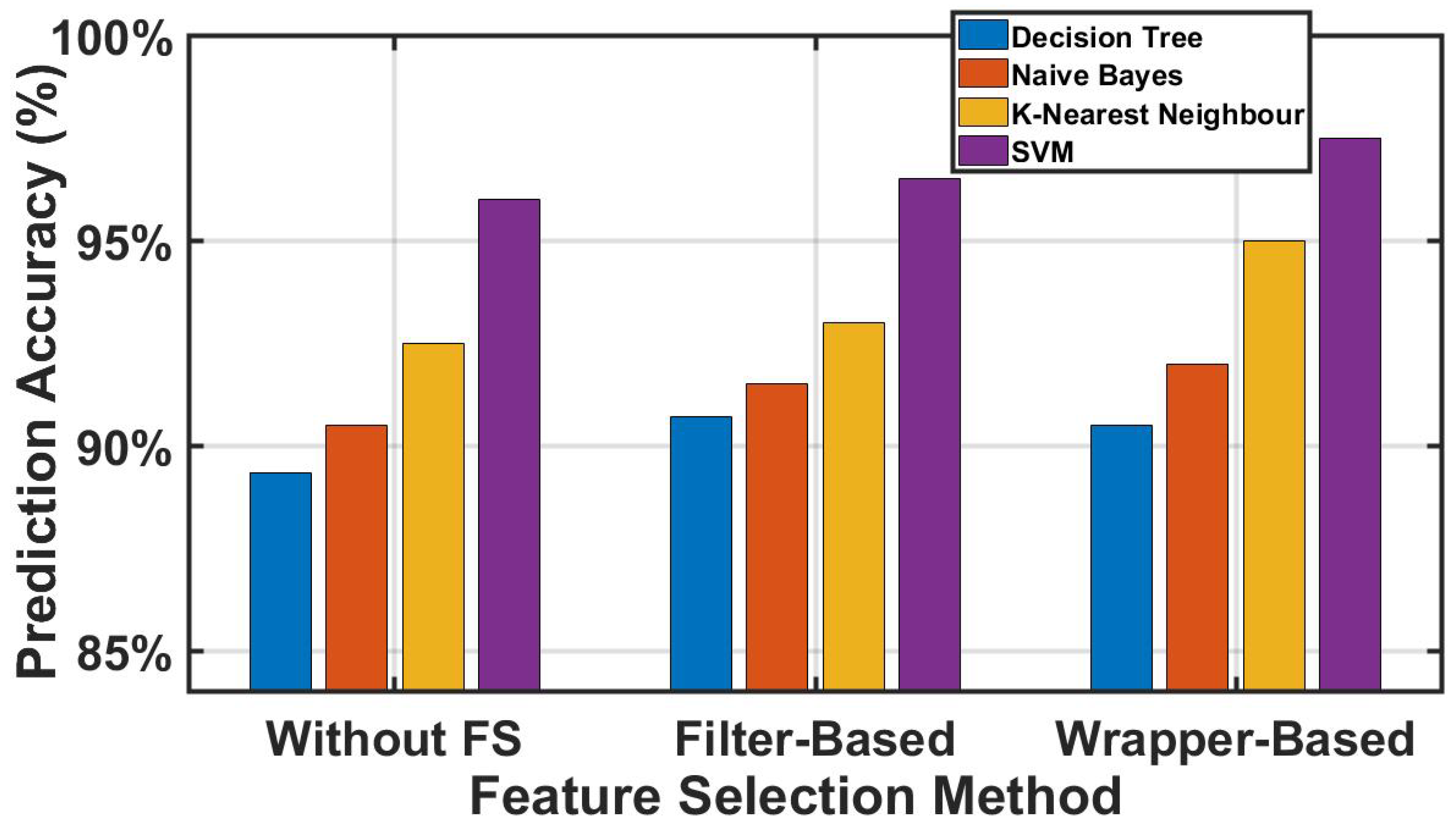
Machine learning model: We propose an IMS call failure prediction model by building eight different ML prediction models to predict whether the ongoing call will succeed/fail based on the aforementioned SIP features (Section 6). We compare four different ML classifiers: decision tree, naive Bayes, K-Nearest Neighbor (KNN) and SVM with using two feature selection methods. The feature selection methods are; (i) the Filter Selection method using the ReliefF algorithm and (ii) the Wrapper Model using the Slime Mould Algorithm (SMA) and Whale Optimization Algorithm (WOA). Predicting the failure enables the operator to prevent the failure by redirecting the call to another radio access technique by initiating the Circuit Switching fallback (CS-fallback) through the 380 SIP error response sent to the handset [12].

(iv)

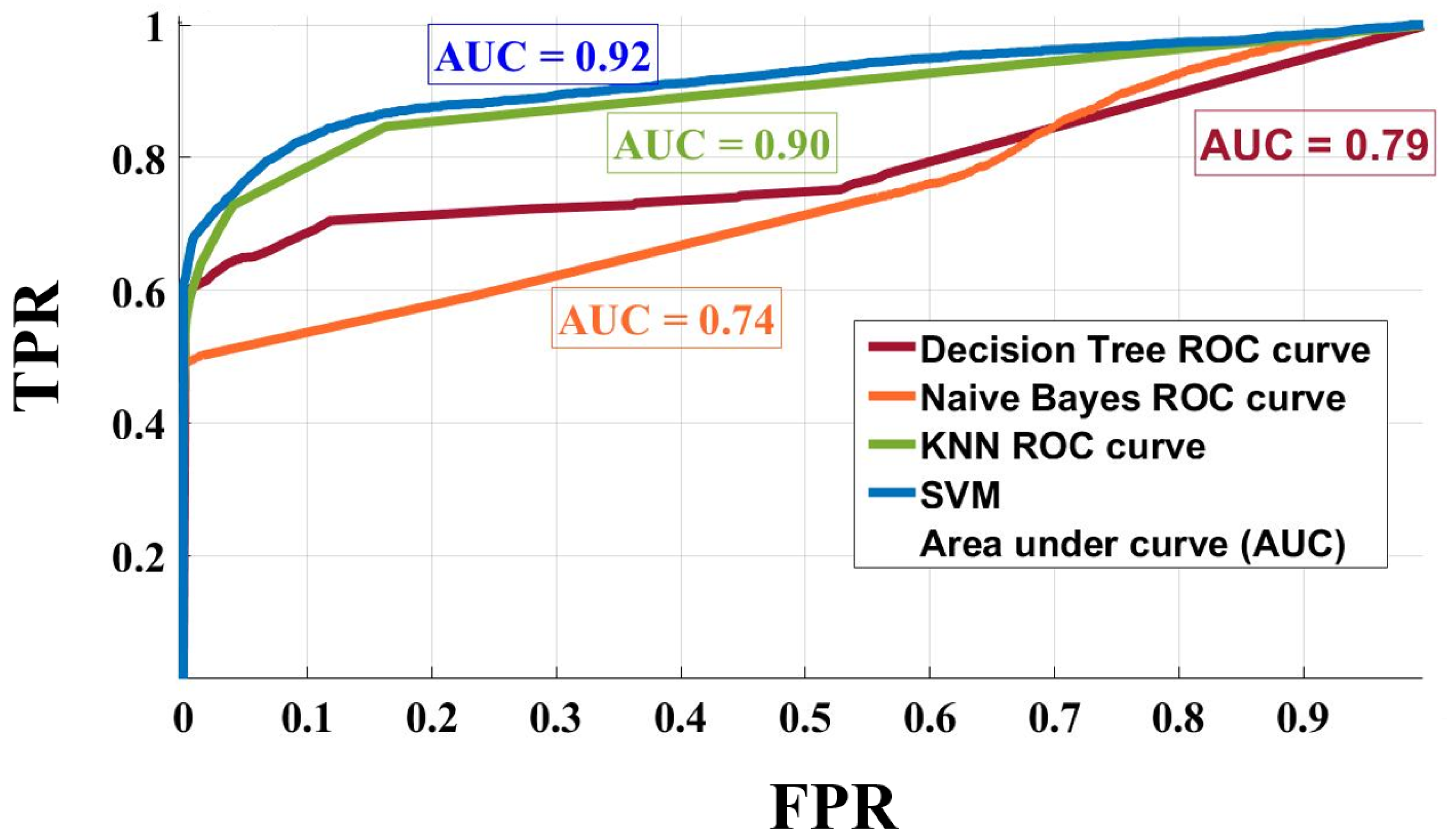
Call failures analysis: The advantage of the model is not limited to call failure prediction, but also to knowing the reason (root causes) behind the failure; more specifically, the multi-factorial reasons by using machine learning, which cannot be obtained using the traditional method (manual tracking of the traces). We perform an analysis for the prediction result (Section 7.3) for the KNN classifier using the Wrapper WOA feature selection algorithm, as it presents the highest prediction accuracy and best ROC performance. This enables us to obtain the call failures’ root causes.

3. VoLTE Call Failure Use Cases

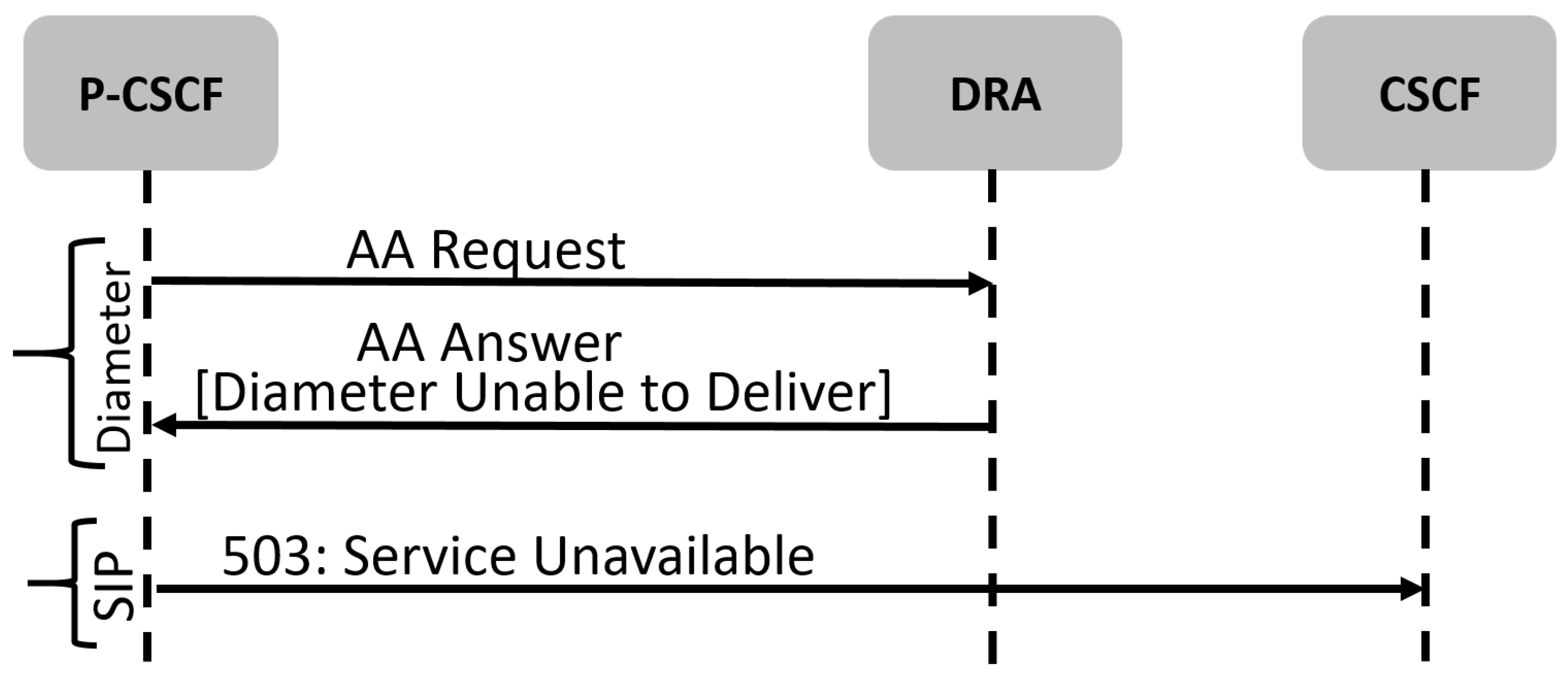
In this section, by using the available dataset, we will discuss three different call failures use cases where failures in Diameter and Real-time Transport Protocol (RTP) protocols lead to a SIP failure response.

1.

Bearer Assignment Failure: This use case includes failure that occurs in the bearer assignment procedure leading to Diameter protocol failure, and then SIP protocol failure. As shown in Figure 1, the invite message was sent from the S-CSCF network node towards P-CSCF as a standard procedure to make a call. The P-CSCF sent an Authentication Authorization Request (AAR) towards PCRF through the Diameter Routing Agent (DRA) to assign the Quality of Service Class Identifier (QCI) bearer to perform the call on the VoLTE Domain. However, DRA responded with a DIAMETER UNABLE TO DELIVER error leading to a successive SIP 503 SERVICE UNAVAILABLE error originating from P-CSCF and sent towards S-CSCF. The root cause was identified as the originating number going out of coverage during performing a call. This leads to a termination request sent from the Packet Data Network Gateway (PDN-GW), deleting the subscriber binding information. As a result, the DRA could not find any binding information for the user and replied with an Diameter UNABLE-To-DELIVER error, as mentioned previously.

2.

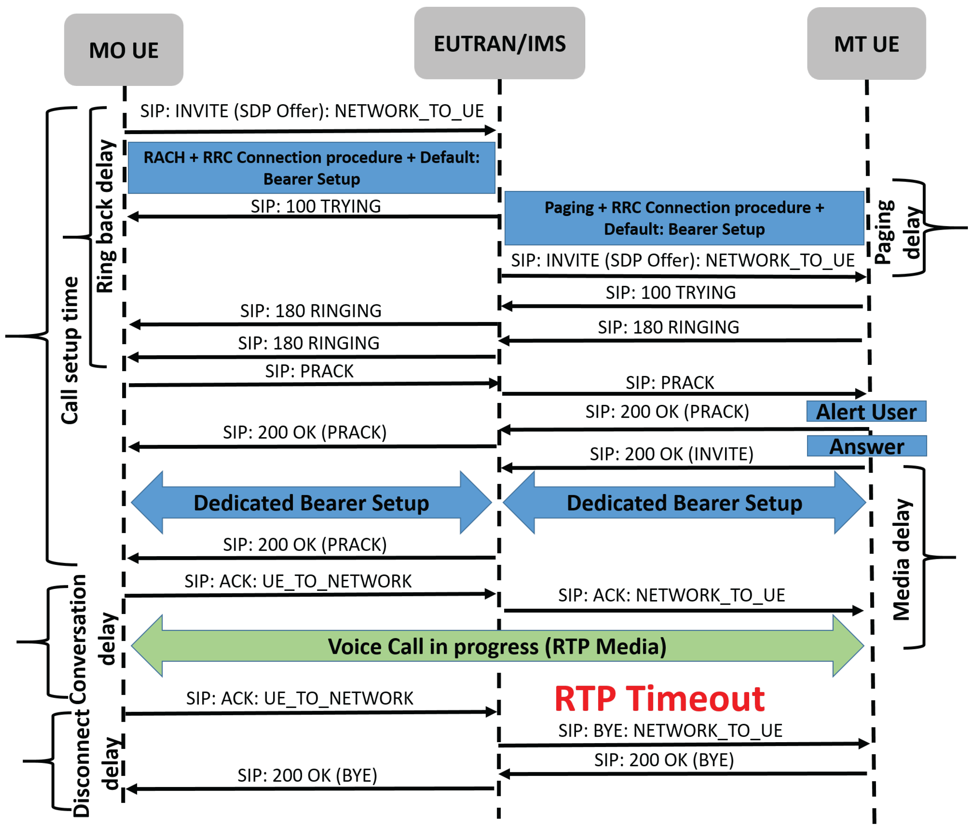
Media Failure: This use case shows a failure that occurred in the opening media channel procedures for a VoLTE call leading to RTP protocol failure then, consecutively, a SIP protocol failure. As shown in Figure 2, the RTP Timeout error in the RTP protocol leads to a CANCEL SIP message containing RTP Timeout, which was sent from the handset side towards P-CSCF, leading to call failure. The RTP Timeout error shows that there was no response received from the IMS Media Gateway side, which led to this call failure.

3.

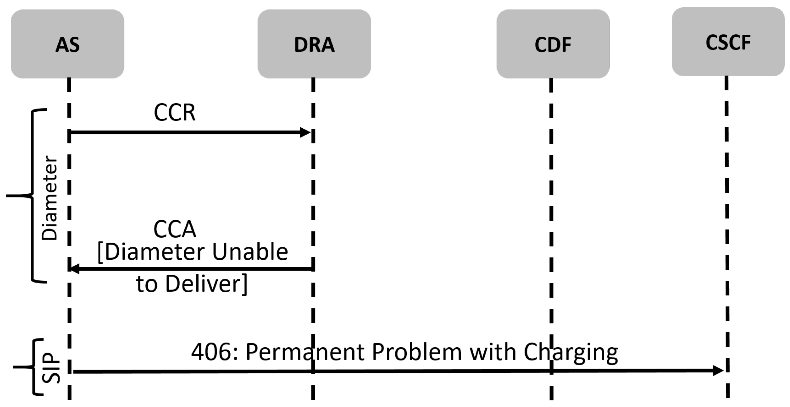
Charging Failure: Figure 3 shows a call SIP/Diameter trace for a charging procedure where a failure occurs in the Diameter protocol, leading to the SIP protocol failure. Before the VoLTE call starts, the Application Server (AS) sends an accounting request to the Charging Data Function (CDF) to open a CDR for the call. This CDR will be used afterward in charging the customer. However, in this use case, the CDF responded with the DIAMETER UNABLE TO DELIVER error. This leads to a SIP 406 NOT ACCEPTABLE error (permanent problem with charging). After investigating the root cause of the failure, it is discovered that the diameter peers between the charging nodes and DRA were down.

From the previously mentioned use cases and according to [13,14,15], we conclude that any failed VoLTE call necessarily leads to a SIP protocol failure response. As a result, monitoring any other protocol (e.g., Diameter, RTP) will show the failures that occur in this protocol. However, by monitoring the SIP protocol, it shows the failures occurring in all the protocols. Therefore, we will use the SIP protocol traces to train the proposed failure prediction ML models, as shown later.

Figure 1. Bearer assignment failure flow.

Figure 1. Bearer assignment failure flow.

Figure 2. IMS media failure flow.

Figure 2. IMS media failure flow.

Figure 3. Diameter charging failure flow.

Figure 3. Diameter charging failure flow.

4. SIP Protocol Analysis

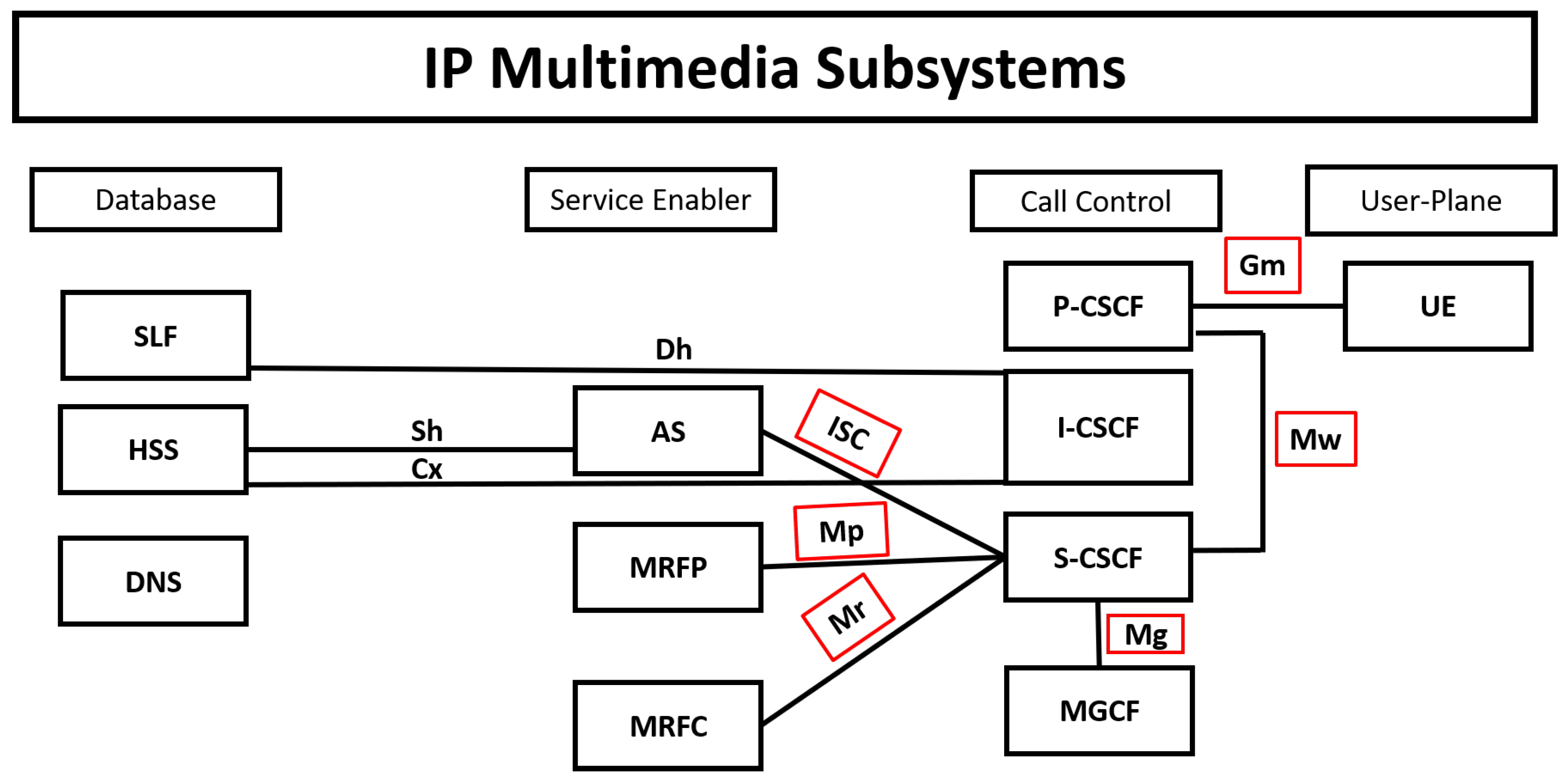
After choosing the SIP Protocol to train the ML model, we need to extract the features from the SIP protocol messages. Then, we will identify the features that we will use to classify the call, whether it succeeded or failed.

A SIP message is either a request from a client to a server or a response from a server to a client [43]. Both Request and Response messages use the basic format stated in [44]. Request and Response messages have the same structure and headers except for two headers that are different [43]: Request-Line and Status-Line headers. The SIP messages are sent over specific interfaces inside the IMS network.

4.1. SIP Interfaces

The first step for building our dataset is to identify the source that generates this data. Therefore, we monitored the IMS interfaces to collect all messages that are related to SIP protocol inside the IMS domain. Figure 4 shows the IMS architecture, and the monitored SIP interfaces are highlighted in red. The Interfaces are mentioned below:

• Mw Interface: The interface between S-CSCF/I-CSCF (Interrogating Call Session Control Function) and P-CSCF;
• Gm Interface: The interface between Subscriber (Handset) and P-CSCF;
• Mg Interface: The interface between Mobile Switching Center (MSC) (circuit switching domain) and I-CSCF;
• ISC Interface: The interface between S-CSCF and the Application server;
• Mj Interface: The interface between the Breakout Gateway Control Function (BGCF) and Media Gateway Controller Function (MGCF);
• Mi Interface: The interface between BGCF and S-CSCF.

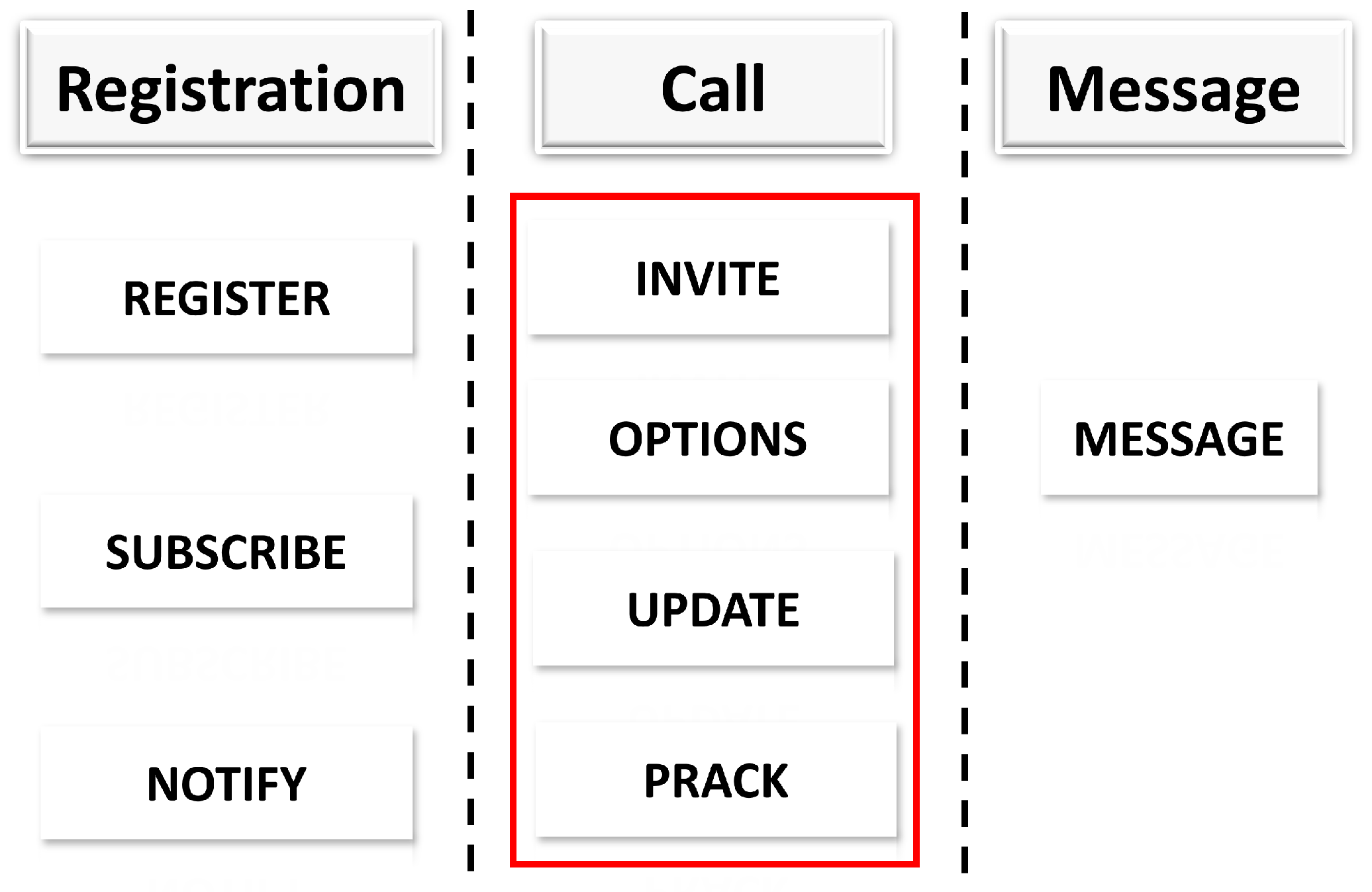
Figure 4. IMS architecture.

Figure 4. IMS architecture.

4.2. SIP Request

SIP Requests have a request-line that shows request type. As shown in Figure 5, the SIP request messages are used in three different call flows: registration, call and message. The SIP request messages are mentioned below, as follows [43];

• REGISTER: Message used for subscriber registration.
• INVITE: Message used for initiating call session.
• OPTIONS: Request used to query Server capabilities
• MESSAGE: Transport instant messaging message.
• SUBSCRIBE: Subscribes to event notification
• REFER: Asks a recipient to issue a SIP request
• UPDATE: Modifies state of a session without changing the state of the dialog and notify the subscriber of a new event.
• CANCEL: Cancels any pending requests.
• PUBLISH: Publishes an event to the server.
• PRACK: Provisional acknowledgment.
• BYE: used in call termination.

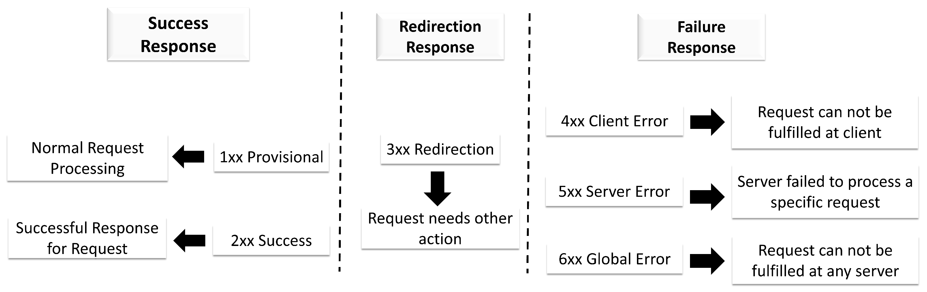
Our focus in this paper is settled on call drops and failures. Therefore, we only chose SIP request types that are present in Mobile Originating (MO)/Mobile Terminating (MT) call flows (highlighted red in Figure 5). We find that Invite, PRACK, CANCEL and BYE SIP requests are present in any successful or failed call. Meanwhile, Refer, Notify and Subscribe SIP requests are present in any successful or failed conference call, specifically [45]. Therefore, we will only monitor these SIP requests.

Figure 5. SIP requests categorization.

Figure 5. SIP requests categorization.

4.3. SIP Response

According to [43], SIP Responses have a Status-Line that shows the SIP response behavior. As shown in Figure 6, SIP responses from 1xx to 3xx are not considered as failures. However, SIP responses from 4xx to 6xx are considered as user, system, and global failures. Although 4xx responses are used for Client errors, some 4xx errors do not resemble a problem as 486 (user busy error). This response is released when a user has an ongoing call. Moreover, 487 (request terminated) usually occurs when a user terminates a call. Therefore, we labeled the responses from 4xx to 6xx as call failures except for 486 and 487.

5. Dataset Description

The CDRs dataset used in this paper is obtained from an Egyptian mobile operator. This dataset provides CDRs for one million originating calls occurring in 24 h. Each CDR is described by 256 fields. Some examples of the dataset CDRs fields are shown in

Table 1. Example of dataset.

Device Model	Audio Codec	Video Codec	Invite Response Time	Answer Time	SRVCC Flag
iphone	101	0	6569	21,656	0
iphone	101	0	3190	13,241	0
Samsung	102	0	3506	28,264	0

.

1.

Device model: The type of the user mobile handset.

2.

Audio codec: Indicates the type of codec used for voice calls. Codec is the abbreviation for coder-decoder or compression-decompression. The two most used codec Narrow-Band Adaptive Multi-Rate (NB-AMR) and Wide-Band AMR (WB-AMR) [46]. The numbers 101 and 102 are defined for WB-AMR and AMR, respectively [46].

3.

Video codec: Indicates the type of codec used for video calls. In the shown example there is no video calls, so all fields of the video codec equal zero. The types of video codecs and the way they are expressed in the CDRs are shown in [46].

4.

Alerting time: The time for the user handset in milliseconds between receiving a 180 ringing SIP response and a 200 ok SIP response.

5.

Answer time: The time of the call in milliseconds.

6.

SRVCC flag: SRVCC is the abbreviation for Single Radio Voice Call Continuity. It is a binary value. It equals one if the user makes a Inter RAT handover from packet data to circuit switched data voice calls. Meanwhile, it equals zero otherwise.

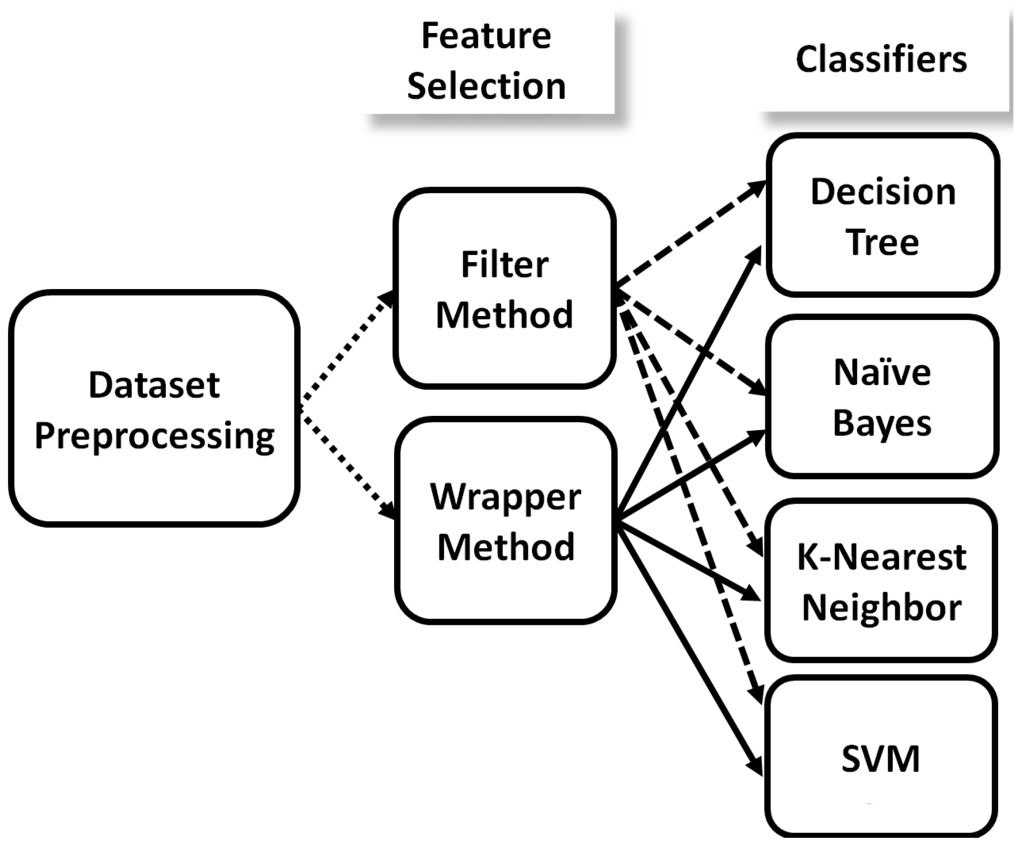
6. Proposed System Model and Machine Learning Prediction Models

The system model is shown in Figure 7. We extract data from the aforementioned SIP interfaces (shown in Figure 4). Then, we apply data to the machine learning model, which is composed of three stages: (i) Data pre-processing, (ii) Feature selection and (iii) Classification. Finally, we analyze the failures to conclude the failure root causes as shown later in Section 7.3. Figure 8 shows the different eight prediction models. We use two different feature selection methods and four classifiers, as discussed in the following.

6.1. Dataset Pre-Processing

Although colossal data are a very beneficial aspect of machine learning, a considerable number of features that do not affect the call state will lead to misleading results. Therefore, we had to do pre-processing in order to filter out data from noise and also to keep Call-Result Relevant features to be used in our classifiers. Pre-processing passed through three stages, we (i) removed noise data, (ii) checked missing data fields in order to remove these CDRs from our data set, and (iii) removed features that describe personal data (Success or fail), as features that contain only one observation and fields that contained user information (e.g., MSISDN, IMSI, IMEI, A-number and B-number, etc.).

6.2. Feature Selection Methods

Feature selection enables a reduction in the computational complexity, as well as the computational time [47]. Feature selection reduces the number of features that will be applied to the classifier model by keeping only features that are more important for call failure/success.

In this work, we will consider two different supervised feature selection methods, namely: the Filter method and Wrapper method combined with four different classifiers. The feature selection methods are as follow;

(i)

Filter method: In the Filter method, the relationship between each input feature and output feature is measured, and each feature is granted a scoring based on statistical tests. Then, the features with a high score are considered. Filter methods are preferred in terms of their easiness in implementation and very low computational time. Several algorithms are present in the Filter method feature selection technique. Algorithms are chosen based on dataset properties such as data dimensions, percentage of redundant, irrelevant features and interaction between features [48]. Since the features present in IMS calls are highly dependent on each other, we use the ReliefF algorithm [49].

(ii)

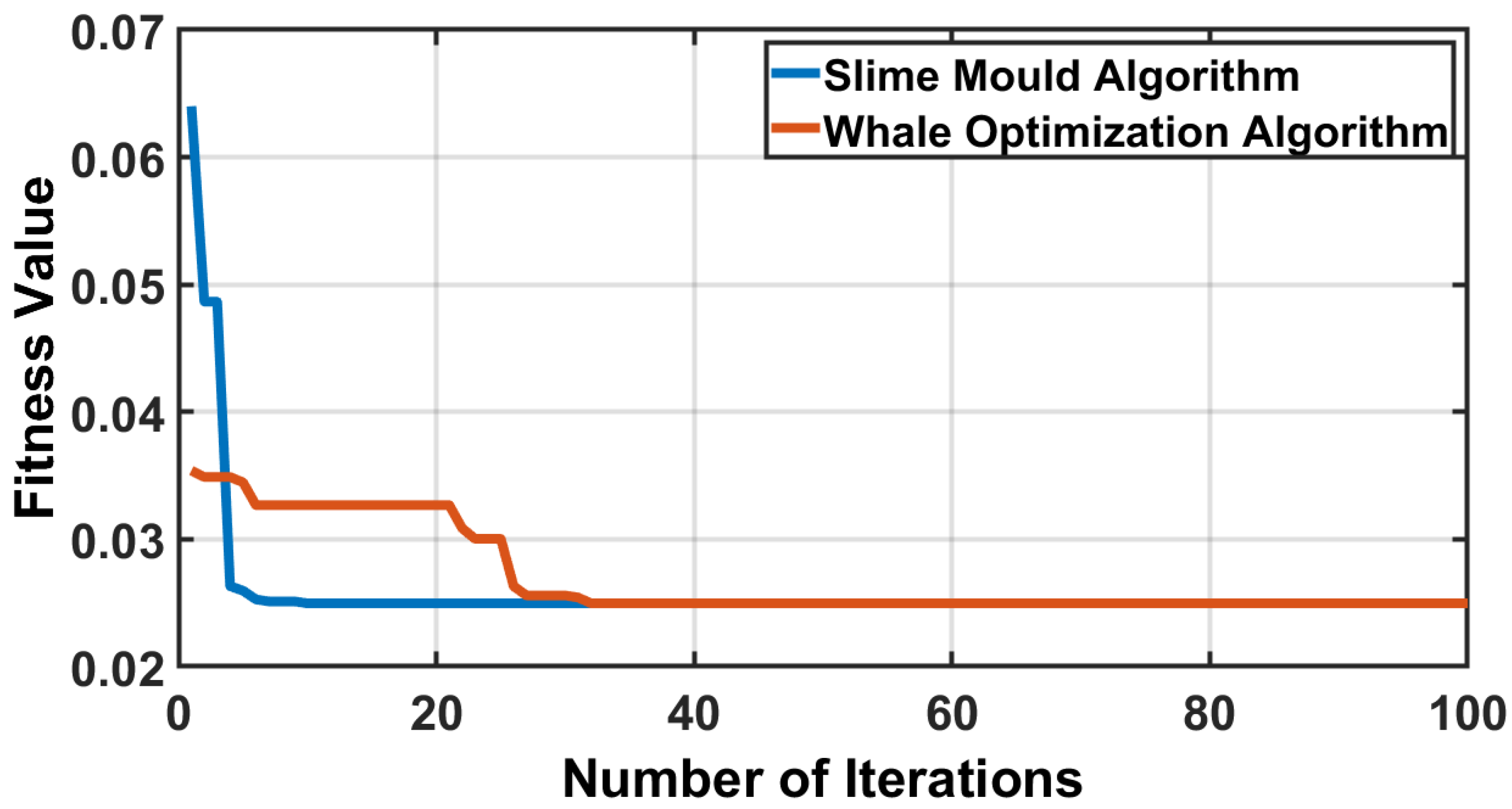
Wrapper method: In the wrapper method, evaluation of features is performed through training a model using ML algorithms, then selecting the best performing features in the model [50]. Moreover, Wrapper methods contain different algorithms. Swarm-based meta-heuristic algorithms have been widely used in several engineering fields due to the fact that they have an advantage over other classes of nature-inspired algorithms [51]. It offers an edge over evaluation-based algorithms by preserving the search space information after each subsequent iteration and fewer operators for successful execution [52]. We have used two of these Swarm Algorithms, WOA and SMA. We have chosen both algorithms for their high capability of solving complex optimization problems compared with other algorithms. In addition, we had a large number of features (256 features) inside our dataset, which led to complex optimization problems.

6.3. Machine Learning Classifiers

We are going to build our model using supervised ML techniques, as the dataset is labeled data. The model predicts whether the ongoing call failed or succeeded (only two values), which is considered as a binary classification. Therefore, we choose four different classification techniques that fit the binary classification: the decision tree, naive Bayes, KNN and SVM.

(i)

Decision Tree: The decision tree classifier is considered as a simple classifier and requires a few parameters. Moreover, the famous advantage of decision tree over other classifiers is its high ability to perform causality assessment (understanding the relation between feature and result). This is on the contrary to black-box modeling techniques, where their internal logic can be challenging to understand.

(ii)

Naive Bayes: The naive Bayes classifier is based on Bayes theorem, which measures the probability of an event occurring given another event.

$$P\left(c\right|x)=\frac{P\left(x\right|c\left)P\right(c)}{P\left(x\right)}$$

(1)

where x is the feature vector; c is the classification variable. It is easy and fast to predict the class of test data set. When the assumption of independence holds, a naive Bayes classifier performs better than other models, such as logistic regression, and it also needs less training data. It performs well in categorical input variables compared to a numerical variable(s), and the data present in CDRs are a categorical data type.

(iii)

K-Nearest Neighbor: We apply KNN classifier since the dataset is sufficiently large and the number of observations is very high compared to the number of features; thus, we went for a low bias and high variance algorithm. Moreover, KNN represents a good option in terms of computational time.

(iv)

SVM: We apply a SVM classifier since they are suitable for binary classification tasks, which is related to and contains elements of non-parametric applied statistics, neural networks and machine learning. It is more efficient in spaces which are high dimensional. It makes adequate use of memory.

6.4. Problem Complexity

The total running time complexity for the decision tree classifier is in the order of O(m.n.log₂n) [53]. Where m is the number of features that describe the data and n is the number of data samples. Meanwhile, the naive Bayes classifier is in the order of O(m.n.²) [54]. Moreover, the total running time complexity for the KNN classifier is in the order of O(m.n.) [55]. Finally, the SVM classifier is in the order of $O\left(n^3\right)$ [56]. This demonstrates that the complexity of the model does not represent an overhead in terms of processing compared to the processing capabilities of the IMS.

7. Results and Analysis

7.1. Evaluation Settings

To evaluate our proposed model, we used MATLAB version R2019a.

In the decision tree classifier, we use a fine tree where the number of splits are 100. In the naive Bayes classifier, for training the data, we used the Kernel predictor distribution, as it improves prediction accuracy compared to the normal distribution. In the KNN classifier, we set K = 10 to give acceptable accuracy without over-fitting. Finally, in SVM, we used the linear kernels, as they give the lowest computational time.

The dataset is divided into a training set and testing set with 60:40 ratios. After validating the model, we compare the different feature selection methods and classifiers regarding the accuracy and the computational time. Finally, we analyze the resulting failures and give important insights into the root causes of the failures.

7.2. Numerical Results

Figure 9 shows the most weighted features concluded by the Filter selection method using the ReliefF algorithm. The features with the positive weights contribute to the successful calls while the features with the negative weights contribute to the failed calls. Moreover, it demonstrated a computational time around 2.2 min.

On the other hand, after applying the Wrapper feature selection method, the number of features concluded were 34 features. The duration taken for running WOA is 30 min and 34 s in 100 iterations. Meanwhile, the duration taken for SMA is 20 min and 40 s in 100 iterations. Moreover, WOA reached a fitness value of 0.025 while SMA reached a fitness value of 0.024, as shown in Figure 10.

By comparing the two feature selection methods, the wrapper method selects fewer features with higher computational times.

As shown in Figure 11, the prediction accuracy of the Decision Tree classifier reached 90.7% using the Wrapper selection method, while it reached 90.5% using the Filter selection method. This low prediction accuracy is due to the multicollinearity problem, as the decision tree makes no assumptions on relationships between features. However, in IMS, there is a strong relation between the features that lead to a call failure/call drop.

For naive Bayes, the prediction accuracy reached around 92% accuracy for the Wrapper feature selection method and 91.5% for the Filter feature selection method. This can be explained by the fact that naive Bayes assign zero probability to any prediction that does not have a specific value. This leads to the removal of any calls that have an empty data in the dataset traces. Moreover, this is the main drive behind the low prediction accuracy obtained compared to the KNN.

In KNN, the prediction accuracy of 95% is achieved by using Wrapper feature selection method. Meanwhile, it reaches 93% by using filter feature selection method. The high accuracy of the KNN classifier is due to the fact that the KNN takes into consideration the correlation between the features, and the used dataset has a high dependency between its features.

In SVM, the highest prediction accuracy of 97.5% is achieved by using the Wrapper feature selection method. Meanwhile, by using filter feature selection method it reaches 96.8%. Figure 11 shows that the Wrapper selection method outperforms the Filter selection method in terms of accuracy when combined with any of the four classifiers. This occurred due to the high capability of Swarm Algorithms that are present in Wrapper methods to solve complex problems, and this condition meets our dataset specs. Moreover, the main disadvantage of the filter selection methods is ignoring the interaction between features, so it considers each feature specifically and IMS CDRs contain highly interacted data; thus, this, explicitly, is the main reason beyond better performance. Moreover, we evaluate the performance of the four classifiers without using feature selection. The prediction accuracies for decision tree, naive Bayes, KNN and SVM are 90.5%, 92% and 95% and 96%, respectively. This shows that each classifier reached its lowest prediction accuracy when it does not use feature selection.

SVM shows the highest prediction accuracy; however, in some cases, prediction accuracy is not reliable. In this case study, our data set does not contain equal distribution for successful and failed calls, as successful calls represent the higher percentage. Therefore, it might have happened that SVM shows the highest prediction accuracy due to its right prediction of only successful calls. In order to evaluate the model with the highest prediction accuracy (SVM), we are going to use the confusion matrix and Receiver Operating Characteristic (ROC).

As shown in Figure 12, the confusion matrix for the SVM classifier shows the prediction results, as follows;

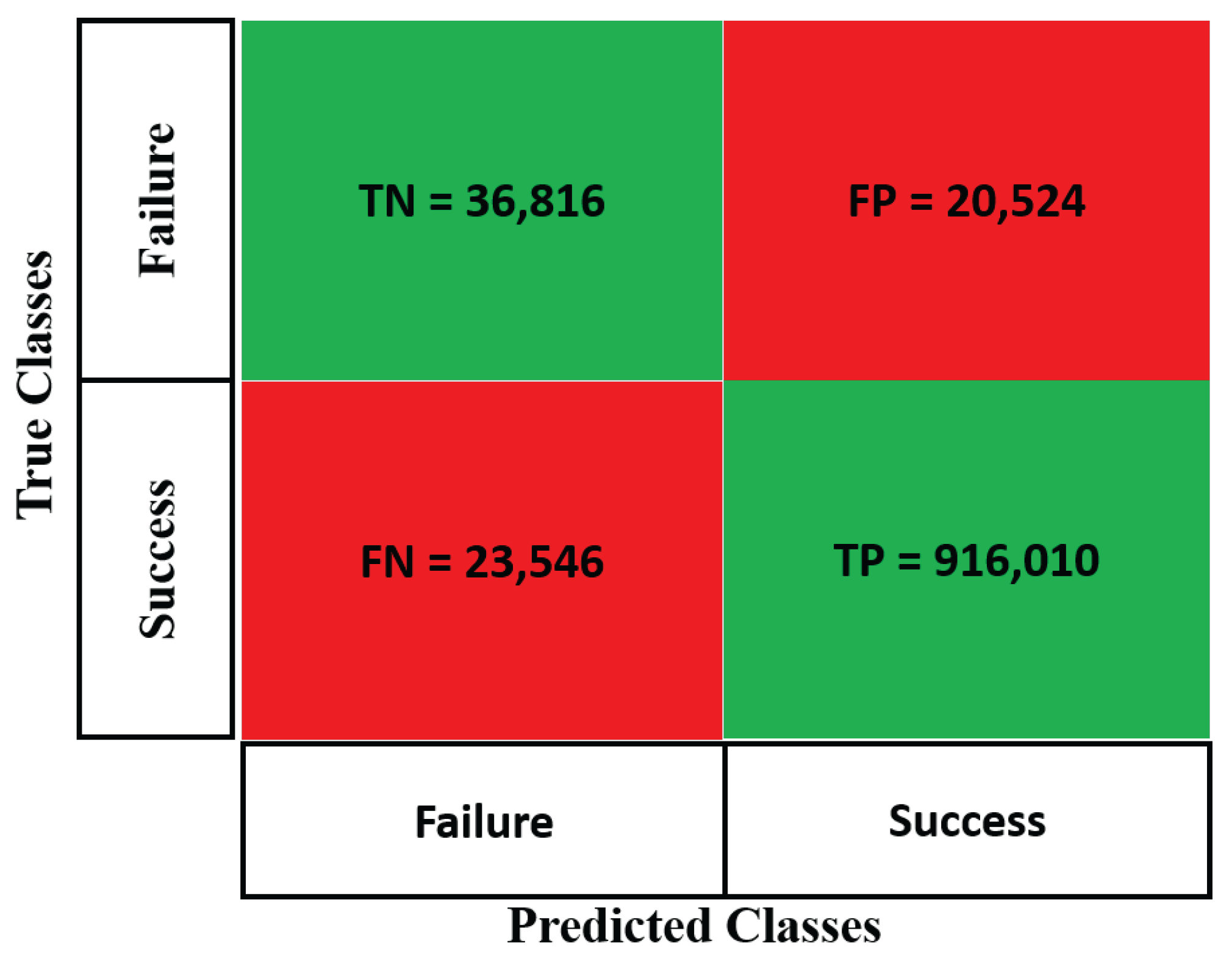
• True Positive (TP): Successful calls rightly predicted as a success (bottom right).
• True Negative (TN): Failed calls rightly predicted as failure (top left).
• False Negative (FN): Successful calls wrongly predicted as failure (bottom left).
• False Positive (FP): Failed calls wrongly predicted as successful calls (top right).

It is shown that the FP is relatively low compared to the TN, indicating that the proposed model can predicate a high percentage of the failures. Moreover, we can calculate the True Positive Rate (TPR) and the False Positive Rate (FPR), as follows;

$$TPR=\frac{TP}{TP+FN}=\frac{\mathrm{916,010}}{\mathrm{916,010}+\mathrm{23,546}}=0.975$$

(2)

$$FPR=\frac{FP}{FP+TN}=\frac{\mathrm{20,524}}{\mathrm{20,524}+\mathrm{36,816}}=0.43$$

(3)

As shown in Figure 13, the ROC curve shows the confusion matrix result on all classification thresholds, where the x-axis is the FPR and the y-axis is the TPR. We compare between different classifiers with measuring the Area Under the Curve (AUC); the classifier with the highest AUC shows the best performance in classification, as it has the highest variance between FPR and TPR over all classification thresholds. Although the naive Bayes has a better prediction accuracy than the decision tree, the later classifier demonstrates better performance in distinguishing between the failure and success calls. The decision tree has a higher AUC than naive Bayes, where the AUC of naive Bayes is 0.74 while the AUC of the decision tree is 0.79.

In order to implement the proposed technique in a real network, first, the data is collected by identifying the SIP interfaces that should be monitored in IMS, as shown in Figure 4 (red highlighted parts). Then, we tapped on these interfaces using probes to collect and assemble SIP messages generated. Second, we ran the model on the IMS virtual machine. Third, an analysis was conducted to obtain and conclude the root causes of call failures, as shown in the following section.

7.3. Call Failure Analysis

In this subsection, we interpret the prediction results for the KNN classifier using the Wrapper WOA feature selection algorithm, as it gives the highest prediction accuracy and best ROC performance. This enables us to get the call failures’ root causes, taking into consideration the following points:

• Firstly, the root causes depend on the dataset (CDRs). Therefore, applying different datasets leads to different root causes.
• Secondly, we had to make sure that the dataset was extracted in a normal day time without any anomaly behavior. For example, when a dataset is extracted during an outage inside the network, the model prediction accuracy turns out to be very high. Since specific features will lead to call failures (e.g., faulty nodes), they could be determined easily in our model, as they will have a very high weight relative to other features. Therefore, the prediction accuracy, in this case, is not reliable.
• Thirdly, we are tackling problems that occur due to multi-factorial reasons and are hardly detected using the traditional way (single trace analysis). In contrast, they can be detected using ML Algorithms.

Based on the call failures analysis, the root causes can be illustrated as follows;

• Failures that occur for VoLTE calls that suffered from the Single Radio Voice Call Continuity (SRVCC) are more significant than the normal VoLTE calls without SRVCC.
• When SRVCC occurs through specific P-CSCF IPs, subscriber suffers from call failures with a percentage reaching 99%. This is a case where the failure is due to multifactorial reasons (P-CSCF IP and SRVCC).
• Specific 5 Tracking Area Identities (TAIs) in the network contribute to a higher percentage of call failures rather than other TAIs.
• The calls where the originating user is using VoLTE and the terminating user is using circuit switching (e.g., 3G)—or vice versa—fail more than the calls where the originating and terminating users are using VoLTE.
• As the invite response time increase, the probability of a call failure increases.
• Twenty percent of used shortcodes have a failure rate of 100%, which shows that these shortcodes are not working inside the IMS domain.

8. Conclusions

In this work, we proposed VoLTE call failures in the IMS network prediction model using machine learning. Firstly, we analyzed different call failure use cases obtained from an Egyptian mobile operator. The analysis demonstrated that the failure in any communication protocol leads to SIP failure. Secondly, we study the SIP protocol to extract the features used to classify the calls either as failures or successes. Based on the used dataset, which contains one million SIP CDRs, we built eight different machine learning models using four different classifiers (decision tree, naive Bayes, KNN and SVM) combined with two different feature selection methods (Filter and Wrapper methods). The results demonstrated that the SVM provides the highest prediction accuracy among all the classifiers and the Wrapper selection method is more efficient than the Filter method in terms of the number of the output features and the computational time. Finally, we analyzed the output of the model with a highest prediction accuracy of 97.5% (SVM Classifier combined with Wrapper Method in feature selection) to obtain the call failure root causes; this enables the network operator to reduce the call drops.

References

1. GSMA. Understanding 5G: Perspectives on Future Technological Advancements in Mobile; Technical Report; Groupe Speciale Mobile Association: London, UK, 2014. [Google Scholar]
2. Shehata, M.; Elbanna, A.; Musumeci, F.; Tornatore, M. Multiplexing Gain and Processing Savings of 5G Radio-Access-Network Functional Splits. IEEE Trans. Green Commun. Netw. 2018, 2, 982–991. [Google Scholar] [CrossRef] [Green Version]
3. Liu, G.; Huang, Y.; Chen, Z.; Liu, L.; Wang, Q.; Li, N. 5G Deployment: Standalone vs. Non-Standalone from the Operator Perspective. IEEE Commun. Mag. 2020, 58, 83–89. [Google Scholar] [CrossRef]
4. Teral, S. 5G Best Choice Architecture; White Paper; IHS Markit Technology: London, UK, 2019. [Google Scholar]
5. Brown, G. Service-Based Architecture for 5G Core Networks; Technical Report; Huawei Technologies Co. Ltd.: Shenzhen, China, 2017. [Google Scholar]
6. Park, S.; Cho, H.; Park, Y.; Choi, B.; Kim, D.; Yim, K. Security problems of 5G voice communication. In Proceedings of the 21st International Conference on Information Security Applications (WISA), Jeju Island, Korea, 26–28 August 2020; pp. 403–415. [Google Scholar]
7. 3GPP. IP Multimedia Subsystem (IMS), Version 16.6.0 ed; Technical Specification (TS) 23.228, 3rd Generation Partnership Project (3GPP); 3GPP: Sophia Antipolis, France, 2021. [Google Scholar]
8. Huawei Technologies Co. Ltd. Vo5G Technical White Paper; Technical Report; Huawei Technologies Co. Ltd.: Shenzhen, China, 2018. [Google Scholar]
9. Asghar, A.; Farooq, H.; Imran, A. Self-Healing in Emerging Cellular Networks: Review, Challenges, and Research Directions. IEEE Commun. Surv. Tutorials 2018, 20, 1682–1709. [Google Scholar] [CrossRef]
10. GSMA. 5G Implementation Guidelines: NSA Option 3, Version 14.2.2 ed; Technical Report; Groupe Speciale Mobile Association: London, UK, 2017. [Google Scholar]
11. GSMA. VoLTE Description and Implementation Guideline, Version 2.0 ed; Technical Report; Groupe Speciale Mobile Association: London, UK, 2014. [Google Scholar]
12. 3GPP. IP Multimedia Call Control Protocol Based on Session Initiation Protocol (SIP) and Session Description Protocol (SDP), Version 12.9.0 ed; Technical Specification (TS) 24.229, 3rd Generation Partnership Project (3GPP); 3GPP: Sophia Antipolis, France, 2015. [Google Scholar]
13. Garcia-Martin, M.; Belinchon, M.; Pallares-Lopez, M.; Canales-Valenzuela, C.; Tammi, K. Technical Report: RFC 4740-Diameter Session Initiation Protocol (SIP) Application; IETF: Wilmington, DE, USA, 2006. [Google Scholar]
14. 3GPP. IP Multimedia Subsystem (IMS) Charging, Version 17.1.0 ed; Technical Specification (TS) 32.260, 3rd Generation Partnership Project (3GPP); 3GPP: Sophia Antipolis, France, 2021. [Google Scholar]
15. 3GPP. IP Multimedia Subsystem (IMS); Multimedia Telephony; Media Handling and Interaction; Technical Specification (TS) 26.114, 3rd Generation Partnership Project (3GPP), Version 16.8.2; 3GPP: Sophia Antipolis, France, 2021. [Google Scholar]
16. 3GPP. Cx and Dx Interfaces Based on the Diameter Protocol; Protocol Details, Version 11.0.0 ed; Technical Specification (TS) 29.229, 3rd Generation Partnership Project (3GPP); 3GPP: Sophia Antipolis, France, 2011. [Google Scholar]
17. Kibria, M.G.; Nguyen, K.; Villardi, G.P.; Zhao, O.; Ishizu, K.; Kojima, F. Big data analytics, Machine Learning, and Artificial Intelligence in Next-Generation Wireless Networks. IEEE Access 2018, 6, 32328–32338. [Google Scholar] [CrossRef]
18. Jiang, C.; Zhang, H.; Ren, Y.; Han, Z.; Chen, K.C.; Hanzo, L. Machine Learning Paradigms for Next-Generation Wireless Networks. IEEE Wirel. Commun. 2016, 24, 98–105. [Google Scholar] [CrossRef] [Green Version]
19. Musumeci, F.; Rottondi, C.; Corani, G.; Shahkarami, S.; Cugini, F.; Tornatore, M. A Tutorial on Machine Learning for Failure Management in Optical Networks. J. Light. Technol. 2019, 37, 4125–4139. [Google Scholar] [CrossRef] [Green Version]
20. Tóthfalusi, T.; Varga, P. Assembling SIP-Based VoLTE Call Data Records Based on Network Monitoring. Telecommun. Syst. 2018, 68, 393–407. [Google Scholar] [CrossRef]
21. Ali, A.; Alshamrani, M.; Kuwadekar, A.; Al-Begain, K. Evaluating SIP Signaling Performance for VoIP over LTE Based Mission-Critical Communication Systems. In Proceedings of the 9th International Conference on Next Generation Mobile Applications, Services and Technologies (NGMAST), Cambridge, UK, 9–11 September 2015; pp. 199–205. [Google Scholar]
22. Bensalah, F.; El Hamzaoui, M.; Bahnasse, A.; El kamoun, N. Behavior Study of SIP on IP Multimedia Subsystem Architecture MPLS as Transport Layer. Int. J. Inf. Technol. 2018, 10, 113–121. [Google Scholar] [CrossRef]
23. Khiat, A.; El Khaili, M.; Bakkoury, J.; Bahnasse, A. Study and evaluation of voice over IP signaling protocols performances on MIPv6 protocol in mobile 802.11 network: SIP and H. 323. In Proceedings of the International Symposium on Networks, Computers and Communications (ISNCC), Marrakech, Morocco, 16–18 May 2017; pp. 1–8. [Google Scholar]
24. Hyun, J.; Li, J.; Im, C.; Yoo, J.H.; Hong, J.W.K. A VoLTE Traffic Classification Method in LTE Network. In Proceedings of the 16th Asia-Pacific Network Operations and Management Symposium (APNOMS), Hsinchu, Taiwan, 17–19 September 2014; pp. 1–6. [Google Scholar]
25. Hsieh, W.B.; Leu, J.S. Implementing a secure VoIP communication over SIP-based networks. Wirel. Netw. 2018, 24, 2915–2926. [Google Scholar] [CrossRef]
26. Abualhaj, M.M.; Al-Tahrawi, M.M.; Al-Khatib, S.N. Performance evaluation of VoIP systems in cloud computing. J. Eng. Sci. Technol. 2019, 14, 1398–1405. [Google Scholar]
27. Bega, D.; Gramaglia, M.; Banchs, A.; Sciancalepore, V.; Costa-Pérez, X. A Machine Learning Approach to 5G Infrastructure Market Optimization. IEEE Trans. Mob. Comput. 2019, 19, 498–512. [Google Scholar] [CrossRef]
28. Fourati, H.; Maaloul, R.; Chaari, L. A Survey of 5G Network Systems: Challenges and Machine Learning Approaches. Int. J. Mach. Learn. Cybern. 2021, 12, 385–431. [Google Scholar] [CrossRef]
29. Ma, B.; Guo, W.; Zhang, J. A Survey of Online Data-Driven Proactive 5G Network Optimisation Using Machine Learning. IEEE Access 2020, 8, 35606–35637. [Google Scholar] [CrossRef]
30. Chernogorov, F.; Chernov, S.; Brigatti, K.; Ristaniemi, T. Sequence-Based Detection of Sleeping Cell Failures in Mobile Networks. Wirel. Networks 2015, 22, 2029–2048. [Google Scholar] [CrossRef] [Green Version]
31. Manzanilla-Salazar, O.; Malandra, F.; Sansò, B. eNodeB Failure Detection from Aggregated Performance KPIs in Smart-City LTE Infrastructures. In Proceedings of the 15th International Conference on the Design of Reliable Communication Networks (DRCN), Coimbra, Portugal, 19–21 March 2019; pp. 51–58. [Google Scholar]
32. Mulvey, D.; Foh, C.H.; Imran, M.A.; Tafazolli, R. Cell Coverage Degradation Detection using Deep Learning Techniques. In Proceedings of the 9th International Conference on Information and Communication Technology Convergence (ICTC), Jeju Island, Korea, 17–19 October 2018; pp. 441–447. [Google Scholar]
33. Takeshita, K.; Yokota, M.; Nishimatsu, K. Early Network Failure Detection System by Analyzing Twitter Data. In Proceedings of the IFIP/IEEE International Symposium on Integrated Network Management (IM), Bordeaux, France, 18–20 May 2015; pp. 279–286. [Google Scholar]
34. Riihijarvi, J.; Mahonen, P. Machine Learning for Performance Prediction in Mobile Cellular Networks. IEEE Comput. Intell. Mag. 2018, 13, 51–60. [Google Scholar] [CrossRef]
35. Sultan, K.; Ali, H.; Zhang, Z. Call Detail Records Driven Anomaly Detection and Traffic Prediction in Mobile Cellular Networks. IEEE Access 2018, 6, 41728–41737. [Google Scholar] [CrossRef]
36. Hussain, B.; Du, Q.; Ren, P. Semi-Supervised Learning Based Big Data-Driven Anomaly Detection in Mobile Wireless Networks. China Commun. 2018, 15, 41–57. [Google Scholar] [CrossRef]
37. Krevatin, I.; Presečki, Ž.; Gudelj, M. Improvements in failure detection for emergency service centers in IMS network. In Proceedings of the 38th International Convention on Information and Communication Technology, Electronics and Microelectronics (MIPRO), Jeju Island, Korea, 26–28 August 2015; pp. 496–500. [Google Scholar]
38. Chen, W.E.; Tseng, L.Y.; Chu, C.L. An Effective Failure Recovery Mechanism for SIP/IMS Services. Mob. Networks Appl. 2017, 22, 51–60. [Google Scholar] [CrossRef]
39. Przybysz, H.; Forsman, T.; Lövsén, L.; Blanco, G.B.; Rydnell, G.; Johansson, K. Failure Recovery in an IP Multimedia Subsytem Network. Telefonaktiebolaget L M Ericsson (publ) Patent EP2195995B1, 6 April 2011. [Google Scholar]
40. Przybysz, H.; Vergara, M.C.B.; Forsman, T.; Schumacher, A. Failure Recovery in an IP Multimedia Subsytem Network. Telefonaktiebolaget L M Ericsson (publ) Patent WO2009039890A1, 2 April 2009. [Google Scholar]
41. Raza, M.T.; Lu, S. Uninterruptible IMS: Maintaining Users Access During Faults in Virtualized IP Multimedia Subsystem. IEEE J. Sel. Areas Commun. 2020, 38, 1464–1477. [Google Scholar] [CrossRef]
42. Chen, X.; Zhou, J.; Liu, K. VoLTE problem location method based on big data. Proc. J. Phys. Conf. Ser. 2021, 1828, 012085. [Google Scholar] [CrossRef]
43. Schooler, E.; Rosenberg, J.; Schulzrinne, H.; Johnston, A.; Camarillo, G.; Peterson, J.; Sparks, R.; Handley, M.J. Technical Report: RFC 3261 SIP: Session Initiation Protocol; IEFT: Wilmington, DE, USA, 2002. [Google Scholar] [CrossRef] [Green Version]
44. Resnick, P. Technical Report: RFC 2822 Internet Message Format; IEFT: Wilmington, DE, USA, 2001. [Google Scholar] [CrossRef] [Green Version]
45. Johnston, A.; Levin, O. Technical Report: RFC 4579 Session Initiation Protocol (SIP) Call Control-Conferencing for User Agents; IEFT: Wilmington, DE, USA, August 2006. [Google Scholar] [CrossRef] [Green Version]
46. 3GPP. Universal Mobile Telecommunications System (UMTS); LTE; IP Multimedia Subsystem (IMS); Multimedia Telephony; Media Handling and Interaction; Technical Specification (TS) 26.114, 3rd Generation Partnership Project (3GPP), Version 13.3.0; 3GPP: Sophia Antipolis, France, 2016. [Google Scholar]
47. Mafarja, M.; Mirjalili, S. Whale optimization approaches for wrapper feature selection. Appl. Soft Comput. 2018, 62, 441–453. [Google Scholar] [CrossRef]
48. Bommert, A.; Sun, X.; Bischl, B.; Rahnenführer, J.; Lang, M. Benchmark for filter methods for feature selection in high-dimensional classification data. Comput. Stat. Data Anal. 2020, 143, 106839. [Google Scholar] [CrossRef]
49. Urbanowicz, R.J.; Meeker, M.; La Cava, W.; Olson, R.S.; Moore, J.H. Relief-based feature selection: Introduction and review. J. Biomed. Informatics 2018, 85, 189–203. [Google Scholar] [CrossRef] [PubMed]
50. Corrales, D.C.; Lasso, E.; Ledezma, A.; Corrales, J.C. Feature selection for classification tasks: Expert knowledge or traditional methods? J. Intell. Fuzzy Syst. 2018, 34, 2825–2835. [Google Scholar] [CrossRef]
51. Hussain, K.; Salleh, M.N.M.; Cheng, S.; Shi, Y. On the exploration and exploitation in popular swarm-based metaheuristic algorithms. Neural Comput. Appl. 2019, 31, 7665–7683. [Google Scholar] [CrossRef]
52. Kumar, A.; Bawa, S. Generalized ant colony optimizer: Swarm-based meta-heuristic algorithm for cloud services execution. Computing 2019, 101, 1609–1632. [Google Scholar] [CrossRef]
53. Sani, H.M.; Lei, C.; Neagu, D. Computational complexity analysis of decision tree algorithms. In Proceedings of the International Conference on Innovative Techniques and Applications of Artificial Intelligence, Cambridge, UK, 11–13 December 2018; Springer: Cambridge, UK, 2018; pp. 191–197. [Google Scholar]
54. Zheng, Z. Naive Bayesian classifier committees. In Proceedings Proceedings of the European Conference on Machine Learning, Chemnitz, Germany, 21–23 April 1998; Springer: Berlin/Heidelberg, Germany, 1998; pp. 196–207. [Google Scholar]
55. Cunningham, P.; Delany, S.J. k-Nearest neighbour classifiers-A Tutorial. ACM Comput. Surv. (CSUR) 2021, 54, 1–25. [Google Scholar] [CrossRef]
56. Abdiansah, A.; Wardoyo, R. Time complexity analysis of support vector machines (SVM) in LibSVM. Int. J. Comput. Appl. 2015, 128, 28–34. [Google Scholar] [CrossRef]
Figure 6. SIP responses categorization.
Applsci 12 08378 g006
Figure 7. Proposed system model.
Applsci 12 08378 g007
Figure 8. Proposed machine learning models.
Applsci 12 08378 g008
Figure 9. Filter method: Features weights.
Applsci 12 08378 g009
Figure 10. Wrapper algorithms: Fitness values.
Applsci 12 08378 g010
Figure 11. Prediction accuracy.
Applsci 12 08378 g011
Figure 12. Confusion matrix for SVM classifier.
Applsci 12 08378 g012
Figure 13. ROC curve over all classifiers.
Applsci 12 08378 g013