Article

Experimental Development of Composite Bicycle Frame

1
Department of Mechanics, Biomechanics and Mechatronics, Faculty of Mechanical Engineering, Czech Technical University in Prague, Technická 4, 16000 Praha, Czech Republic
2
Compo Tech PLUS, spol. s r.o., Nová 1316, 34201 Sušice, Czech Republic
*
Author to whom correspondence should be addressed.
Appl. Sci. 2022, 12(16), 8377; https://doi.org/10.3390/app12168377
Submission received: 31 December 2021 / Revised: 31 July 2022 / Accepted: 15 August 2022 / Published: 22 August 2022
(This article belongs to the Special Issue Experimental Mechanics, Instrumentation and Metrology II)

Abstract

:
This article focuses on the development of a carbon composite bicycle frame using various experimental methods of structural analysis. Two types of frame specimen were used. The complete frame specimen was tested in accordance with ISO test load cases with the addition of an ergometer test in order to refine the operational strain envelope of such a frame. Resistive strain gauges and optical Fiber Bragg Grating (FBG) sensors were used for this analysis. The FBG sensors were embedded inside the head tube joints during the manufacturing process. The head connection was designed as a geometrically precise form–connection of wound composite tubes, reinforced with a wrap of high-strength unidirectional carbon tapes and carbon fabrics. Additional structural strength laboratory tests were conducted using simplified frame specimens, in order to evaluate the range of the limit case strain ranges. The digital image correlation method was used for the evaluation of the strain distribution in the head tube area. Resistive strain gauges were used for local strain analysis in critical areas. The acoustic emission method was used to detect structural defects before they could influence the stiffness response of the frame. It was found that the joints of the frame tubes are crucial for the strength and safety of the frame. Therefore, attention was also focused on the strengthening of the head tube joint, and on its experimental verification. A positive effect on the strength of the reinforced frame was found by doubling the thickness of the carbon fabric in the head tube joint area.

1. Introduction

Bicycle frames made from carbon fiber reinforced polymers (CFRP, see Figure 1) are now widely commercially available. Besides prepreg molding technology, composite wound tube technology is the most common method for the manufacture of bicycle frames. In general, the most problematic points of a bicycle frame, which consists of wound structural tubes, are the joints of these structural tubes. One common method of joining the tubes, by using glued sleeve joints, has both performance and visual limitations. These are caused by the technology of the composite manufacturing itself [1], which differs from the traditional manufacturing technology for steel or alloy frames, especially with regard to the service life of the adhesive joints of composite tubes [2]. Therefore, research has focused on joint improvement, by trying to improve the strength of the hand lay-up laminated joints. Structural stress–strain analysis is an integral part of such research and experimental verification is necessary. In order to achieve the optimal design of a bicycle frame, as well as other components such as forks, handlebars, etc., it is essential to have the best possible knowledge of the static and dynamic properties of the frame and other individual components.
These can now be routinely tested in the laboratory. To identify the dynamic parameters of the structures, input–output methods are used [3]. Newer methods combine, for example, the wavelet-transformed representation of system responses with an independent component analysis [4,5]. The static, as well as fatigue tests, need to demonstrate that the bike’s structure has sufficient strength. This must be demonstrated from the stiffness point of view; for example, [6] describes the analysis of the frame stiffness response, and from the fatigue life point of view; for example, [7] describes the fatigue testing of the front carbon fork. The increasing demand to improve the performance of bicycle frames, especially from a safety point of view, necessitates an accurate description of the operational load of the frame. Due to the complexity and cost of such a task, which results from the requirement for small, lightweight and durable experimental equipment, operational measurements are performed only by some bicycle frame manufacturers. The origins of these operational experiments date back to 1968, when the first strain gauge (SG) analysis of pedal-and-crank strain was performed [8]. Today, even operational fatigue analyses are common, where the load operating spectra are measured by strain gauges calibrated to measure force, both for metal frames [9] and for composite frames [10]. However, due to the complexity and cost of operational measurements, bicycle manufacturers mainly focus on numerical simulations. These are created from basic models using beam elements to determine stiffness behavior [11], through the use of shell elements [12], to optimization tasks performed on the composite frame lay-up configuration [13]. The common solutions for laboratory and operational measurements use strain gauge analysis. In addition to bicycle frame testing, they are focused on testing other critical components such as handlebars, pedals and forks. However, experiments which commonly use the electrical strain gauge method for the stress–strain verification of the frame have some crucial disadvantages. A strain gauge cannot be embedded inside the composite lay-up or inside an adhesive joint. Therefore, only the surface strain can be measured. This could be insufficient in a case where a strain analysis of a geometrically complex shape is needed. A structural analysis of the specific layers of composite lay-ups or joints can be performed using Fiber Bragg Grating (FBG) sensor measurement technology, because FBGs are small enough to be placed between the particular filaments [14,15].
Tests of bicycles, including their components, are described in ISO 4210 [16]. The standard is constantly evolving and adapting to emerging cycling trends. Among other things, the EFBE Prüftechnik GmbH testing laboratory in Germany is involved in their development. Tests of the standardized cases described in this article were performed in this testing laboratory. Because this research work focuses only on the bicycle frame, tests are selected from the part of the ISO 4210-6 standard [17], which describes the testing of the frame and fork. The requirements for passing the tests are described in part ISO 4210-2 [18]. The aforementioned regulations for testing bicycle frames prescribe three main types of tests: impact load tests of the frame; fatigue tests of the frame (for example of the test schemes see Table 1); and static stiffness tests of the frame. For the impact tests, the change in wheelbase is evaluated, i.e., the distance between the axles of the front and rear wheels, before and after impact. Standard [18] specifies the permissible permanent deflection. The frame must not show any signs of failure after the impact test and no part of the frame should be separated after the second impact. In order for the composite frame to pass the fatigue tests according to [18], no cracks must appear and the deflection of the force actuator must not be increased by more than 20%. The experience of the International Cycling Federation (UCI) and other independent testing laboratories also shows that these load cases well represent the load on the bicycle, but the level of load should only be considered as the minimum to ensure the safety of the cyclist [19,20].
The following text focuses on fatigue cyclic tests and static stiffness tests. We will experimentally examine the behavior of a composite bicycle frame during standardized load cases. This will be extended via testing on an ergometer in order to expand the operational envelope of the possible frame strains and loads. This will enable us to tune the strength and rigidity of the bicycle frame by strengthening the composite lay-up in the head tube joint area. The behavior of this innovative joint needs to be investigated experimentally, in order to investigate which of the experimental methods is suitable for strain analysis, as well as for the detection of joint or composite tube failure. Embedded FBG strain sensors, supplemented by strain gauges installed on the frame tubes, are used to monitor strain in this critical structural point of the frame. The limits of the behavior of the frame are investigated during the structural strength test, using other experimental methods such as the digital image correlation (DIC) method and the acoustic emission (AE) method. The FEA method was used for local strain analysis in the head tube joint composite lay-up.
Using the above mentioned experimental and computational methods, the main goal of this paper is to examine the head tube joint of a composite bicycle frame in terms of the strain response inside the joint and on its surface, and to improve its strength properties.

2. Experimental Methods

Research work conducted on the composite bicycle frame included a range of tasks: from material experiments to full-scale laboratory testing. The full bicycle frame, including chain stay and seat stay, was used for the purpose of laboratory testing during standardized ISO test cases. Embedded optical FBG strain sensors were used for the local strain analysis of the head tube (HT) joints with the lower frame tube (down tube, DT) and upper frame tube (top tube, TT). Electrical strain gauges were installed on selected places on the surface of the frame for the measuring of nominal strains. The mandatory test cases indicate the minimum operating range, both nominal and local, of the mechanical strain in the head tube joints area with different types of loadings. In the next step, the bicycle built with this instrumented frame was loaded with a pedaling cyclist on an ergometer. Again, measurements of the mechanical strain were obtained from the FBG sensors and strain gauges. Other experimental work was performed using simplified frames, which were made without both chain-stay and seat-stay tubes. This made it possible to compare actual normal operating loads with standardized tests. In these cases, where the front frame triangle was instrumented only with selected strain gauges near the head tube, integrated FBG sensors were not installed. The digital image correlation (DIC) method was used to analyze the deformation of the head tube with the top tube and down tube connections. This method was used for the determination of the local deformation along the line representing the integrated FBG sensor, i.e., in the longitudinal axis of the reinforcing carbon tape. It was also employed for the determination of the local strain extremes in the head tube area. The experimental configuration was supplemented by AE method sensors to detect the initiation of failure in the composite structure or frame tube joints. The experimental flowchart is described in Table 1.

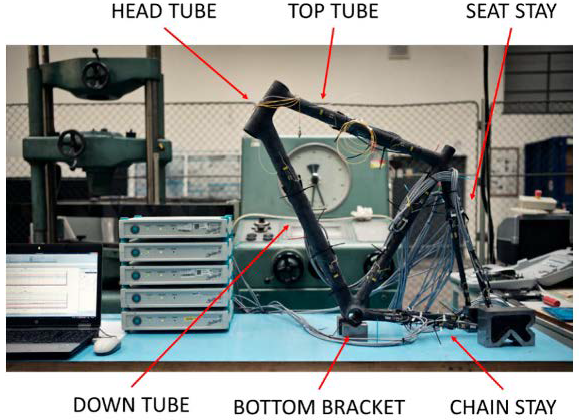
2.1. Composite Bicycle Frame Experimental Configuration

A composite bike frame was made using composite tubes, manufactured by a filament winding technology, as the main structural parts. The technological advantage of this solution is the possibility of winding layers of composite with longitudinally oriented fibers. This includes the application of hybrid compositions of materials; in this case, high-strength (Toray T700 fiber) and high-modulus (Tenax® UMS40 fiber) carbon fibers. In combination with a two-component epoxy resin, a fiber volume fraction in the range of 51–55% was achieved. The tube-to-tube manual lamination method was then used to form the connections of these particular frame tubes, using carbon fabric and unidirectional (UD) tape and epoxy resin matrix. Micro-balloon-filled, two-component epoxy resin was used to complete the shape transitions. The strength of such joints with respect to the hand composite lay-up process may represent a weak point of the frame’s strength. This should be experimentally verified. The composite frame in question is optimized for rigidity and weighs 800 g with a size of 54 cm.
Two bicycle frame specimen types were manufactured. The first one was a complete bicycle frame ready for laboratory tests, and the full-scale test of the complete assembled frame that follows (frame specimen 0, Figure 1). The second specimen type was designed for extended laboratory testing, with the focus on the most loaded joint, which is the connection of the head tube to the down tube and the top tube. For this purpose, simplified frames containing the main frame triangle were made and tested (frame specimens 1, 2, 4, 5, 6 and 7), as shown in Figure 2. Frame specimen 7 differs from the others by the reinforced composite lay-up in the head tube joint area. Additional carbon fabrics were added so that the number of layers was doubled. A bicycle frame of the first type was instrumented with surface-mounted strain gauges and structural FBG sensors. Optical fibers were embedded into the joint connecting the top tube (FBG TT) with the head tube, and the joint connecting the down tube (FBG DT) with the head tube (Figure 3a), directly between the unidirectional carbon filament layers (UD tapes, see Figure 3b). From a safety point of view, these places are critical for the transfer of horizontal forces. The positions and markings of individual electrical and optical strain sensors are marked in the scheme in Figure 4a. Details of the locations of the FBG sensors, FBG TT (Top Tube) and the FBG DT (Down Tube), in the head tube area are shown in Figure 4b. The head tube connection area is then covered with carbon fabric in the last step of the hand lay-up lamination process.

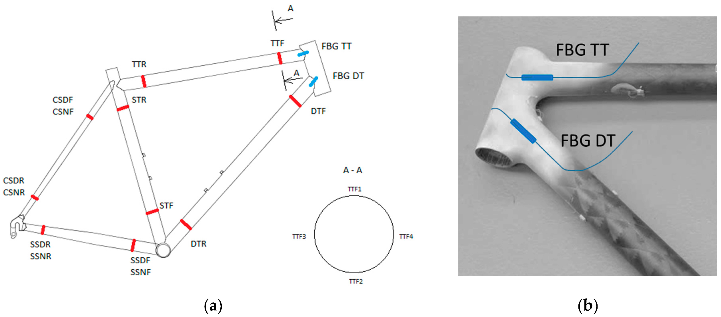
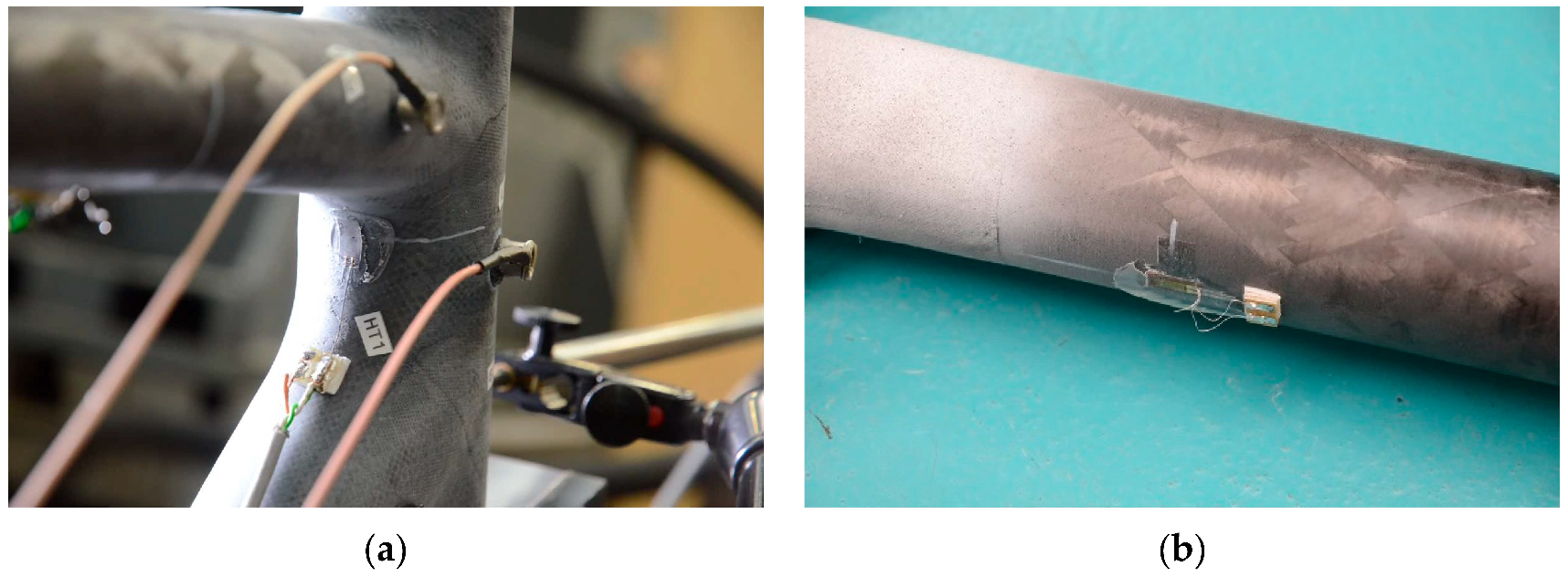
2.2. Fiber Bragg Grating Sensors

Two ORMOCER® coated optical fibers instrumented with one FBG sensor per fiber were used. The surface routing of the fibers was protected using plastic tubes. The mechanical strain indicated by the FBG sensors was measured and evaluated using the Safibra FBGuard optical interrogation system. A measurement error of ±6.1 µm/m was calculated from the maximum wavelength repeatability of the FBGuard device. A more detailed description of the method is provided in Appendix A.1. The properties of both the FBG sensor [21] and the measurement device [22] are shown in Table A1 in Appendix A.1.

2.3. Resistive Strain Gauges

Strain gauges were only installed on the surface of the frame tubes using a methylmetacrylate cold curing adhesive. Two strain gauges on the top tube (TTF location in Figure 4a and Figure 5b) and two on the down tube (DTF location in Figure 4a) are located at the point of the neutral axis of the DT and the TT (from the point of view of the front–rear horizontal loading direction of the frame). One strain gauge was installed on the back side of the HT in an axial direction, as shown in Figure 5a. Linear strain gauges with a resistance of 350 Ohms and a 6 mm long measuring grid were used. Strain gauges were connected to the HBM Spider8 data acquisition device using a quarter bridge connection configuration. A measurement error of ±6 µm/m was calculated from the measurement range and accuracy class of the Spider8 device. A more detailed description of the method is provided in Appendix A.2 The properties of both the strain gauge and the measurement device are shown in Table A2 in Appendix A.2.

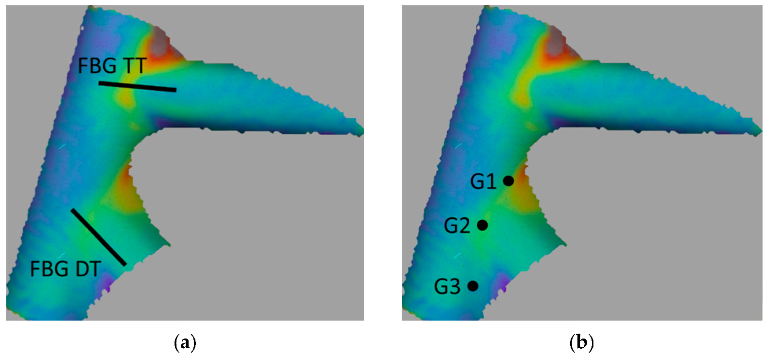
2.4. Digital Image Correlation

A Dantec Dynamics Q400 commercial DIC system equipped with two 16 Mpix digital cameras was used. The position of the measuring set-up close to the bicycle frame provided a resolution of approximately 0.08 mm/px. A thin surface layer of acrylic lacquer (black and white) was sprayed on the specimen to create a random pattern. Istra 4D software was used for data evaluation. Measured displacements were smoothed in the evaluation software by local regression on a kernel grid measuring 9 × 9 px. To compare the measurement methods, the average longitudinal strain was evaluated along the line representing the FBG sensor routing in its sensing area (marked FBG TT, FBG DT, see Figure 6a). The joint of the DT to the HT was chosen as the place of interest, so three circle area gauge objects (marked G1, G2, G3) were created in the joint area for a comparison of frame specimens (see Figure 6b). The comparison provided is presented by mean principal strain 1 as an example of identified behavior. A more detailed description of the method is provided in Appendix A.3.

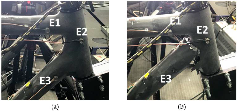
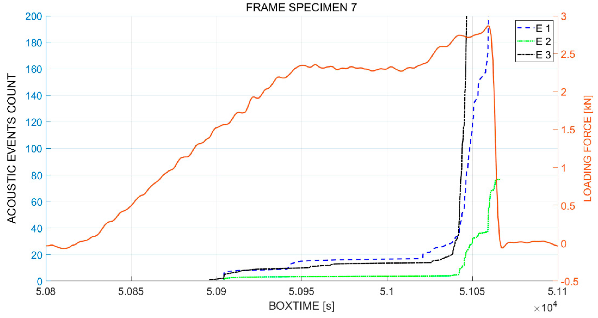
2.5. Acoustic Emission Method

Bicycle frames were equipped with three Dakel IDK-09 piezoelectric sensors, marked E1 (TT location), E2 (HT location) and E3 (DT location), which were attached to the tubes by means of cyanoacrylate adhesive. These sensors were connected to the Dakel Rpety XEDO-AE21 measurement device. The location of the sensors on the frame specimen is shown in Figure 7. A more detailed description of the method is provided in Appendix A.4. The properties of both the acoustic emission sensor and the measurement device are shown in Table A3 in Appendix A.4.

2.6. Experimental Set-Up

In the first phase of the experiments, the bicycle frame (frame specimen 0) was tested in cooperation with the EFBE Prüftechnik GmbH (Waltrop, Germany). The aim was to become thoroughly aware of the behavior of the bike frame in the ISO defined load cases. This was followed by the ergometer test. A simplified bicycle frame (frame specimens 1, 2, 4, 5, 6 and 7) underwent laboratory testing up to the point of structural failure in order to examine the structural strength of the frame.

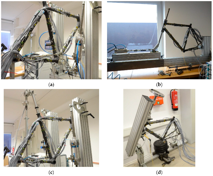
2.6.1. Standardized Load Cases

A set of frame loading procedures was based on the ISO 4210-6 [17] bicycle safety standard, supplemented by specific load cases:
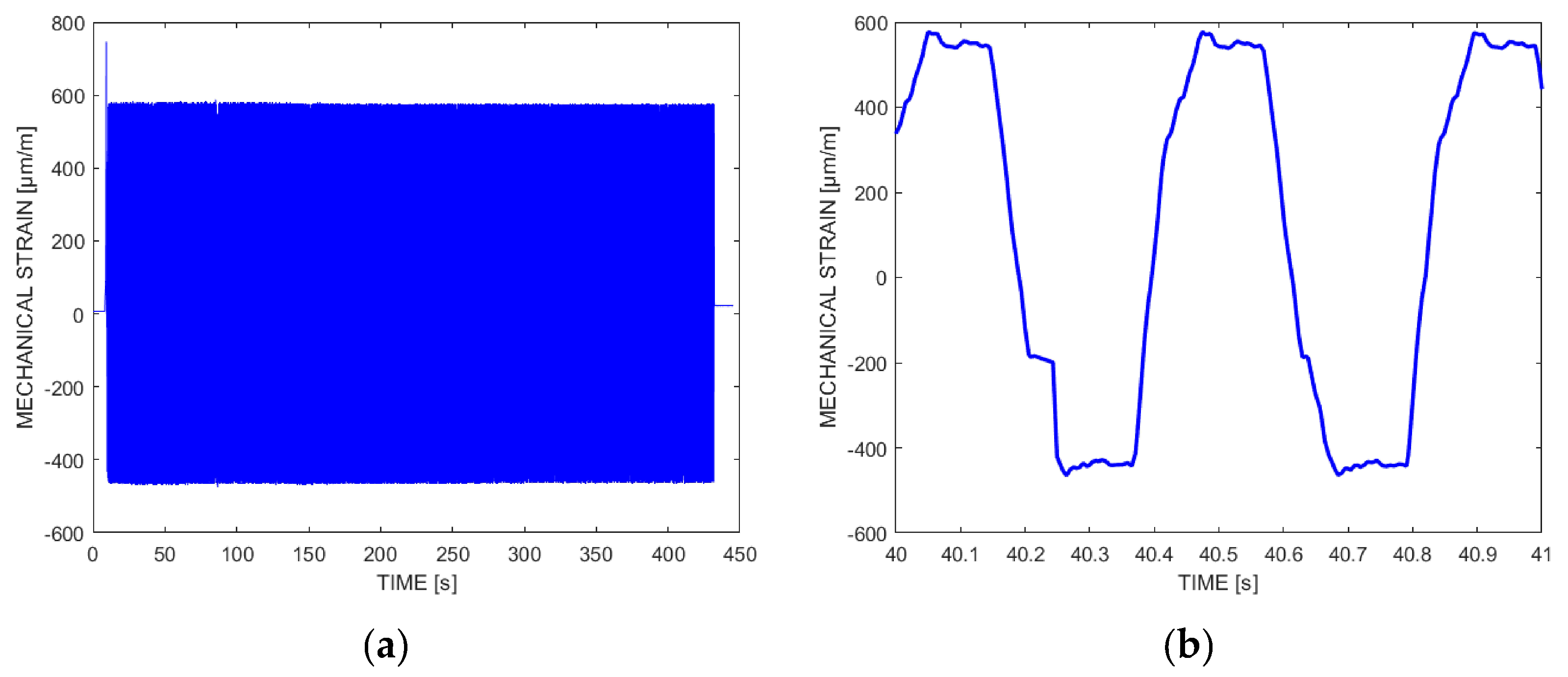
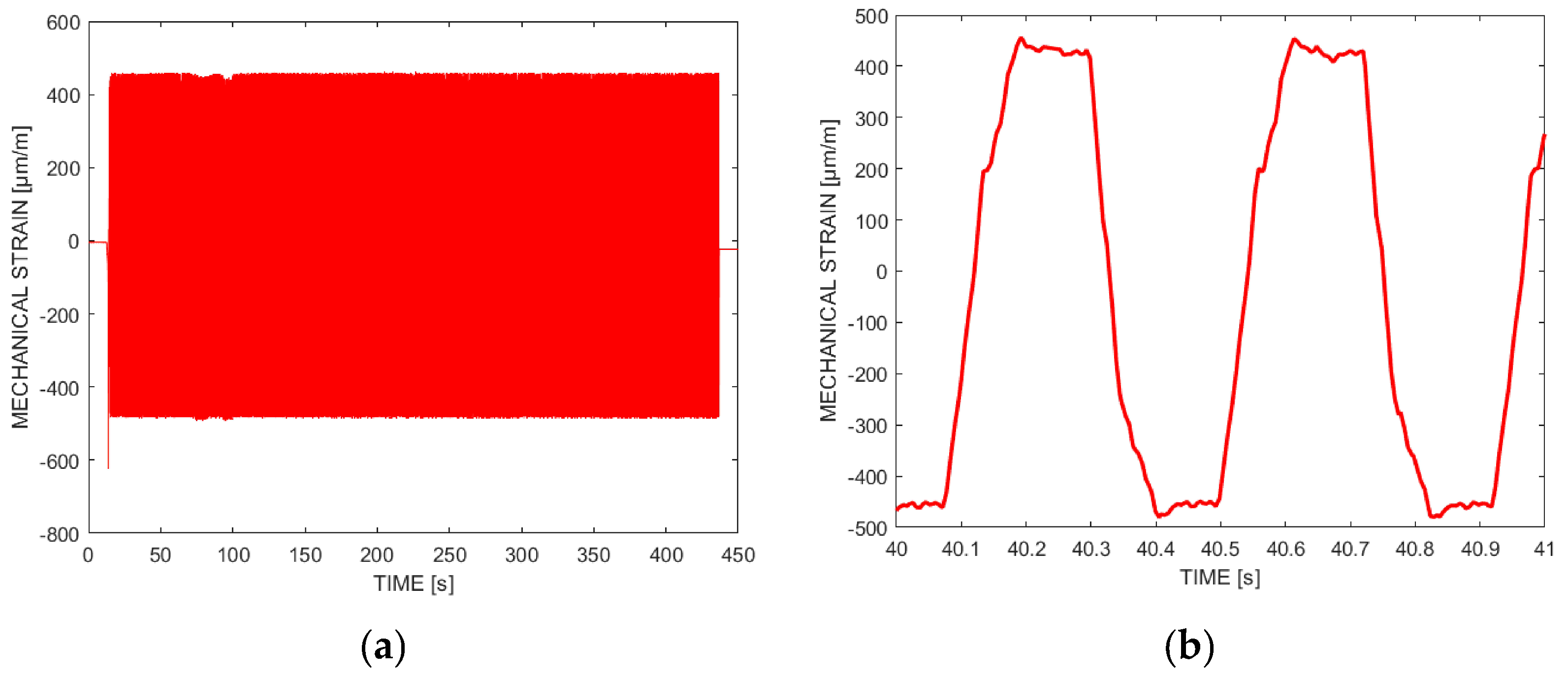
  • Pedal forces (frame is attached through the rear dropouts and loaded by vertical force F = 1100 N through the right crank, load control mode, frequency of cyclic loading f = 2.5 Hz, 1000 cycles, Figure 8a);
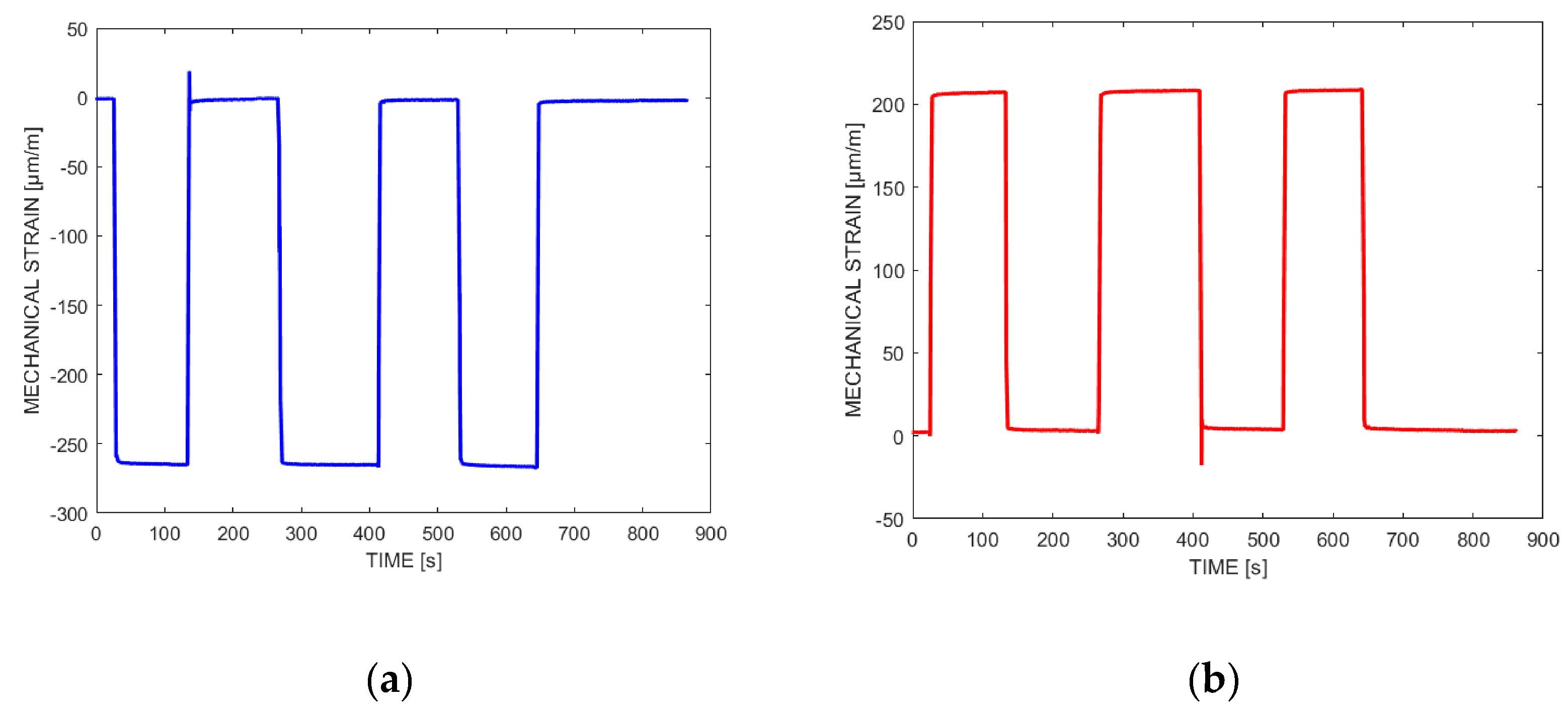
  • Horizontal forces (frame is attached through the rear dropouts, with a front/back horizontal load through the fork, F = 600 N, load control mode, frequency of cyclic loading f = 2.5 Hz, 1000 cycles, see Figure 8b);
  • Vertical forces (frame is attached through the rear dropouts and head tube, with vertical loading through the seat tube, F = 1200 N, load control mode, frequency of cyclic loading f = 2.5 Hz, 1000 cycles, see Figure 8c);
  • Bottom bracket stiffness (frame is attached through the rear dropouts and head tube, with torsional loading through the bottom bracket, F = 756 N, 3 load cycles, see Figure 8d);
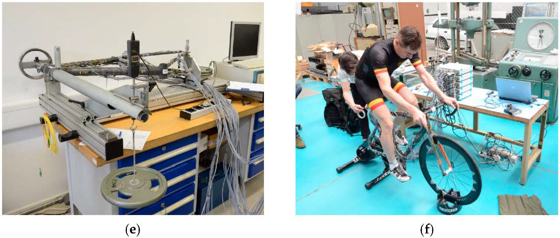
  • Head tube torsion stiffness (frame is attached through the rear dropouts and head tube, torsional loading M = 43.5 Nm is introduced through the equivalent test fork, deformation is measured between the front and rear wheel plane, 3 load cycles, see Figure 8e).

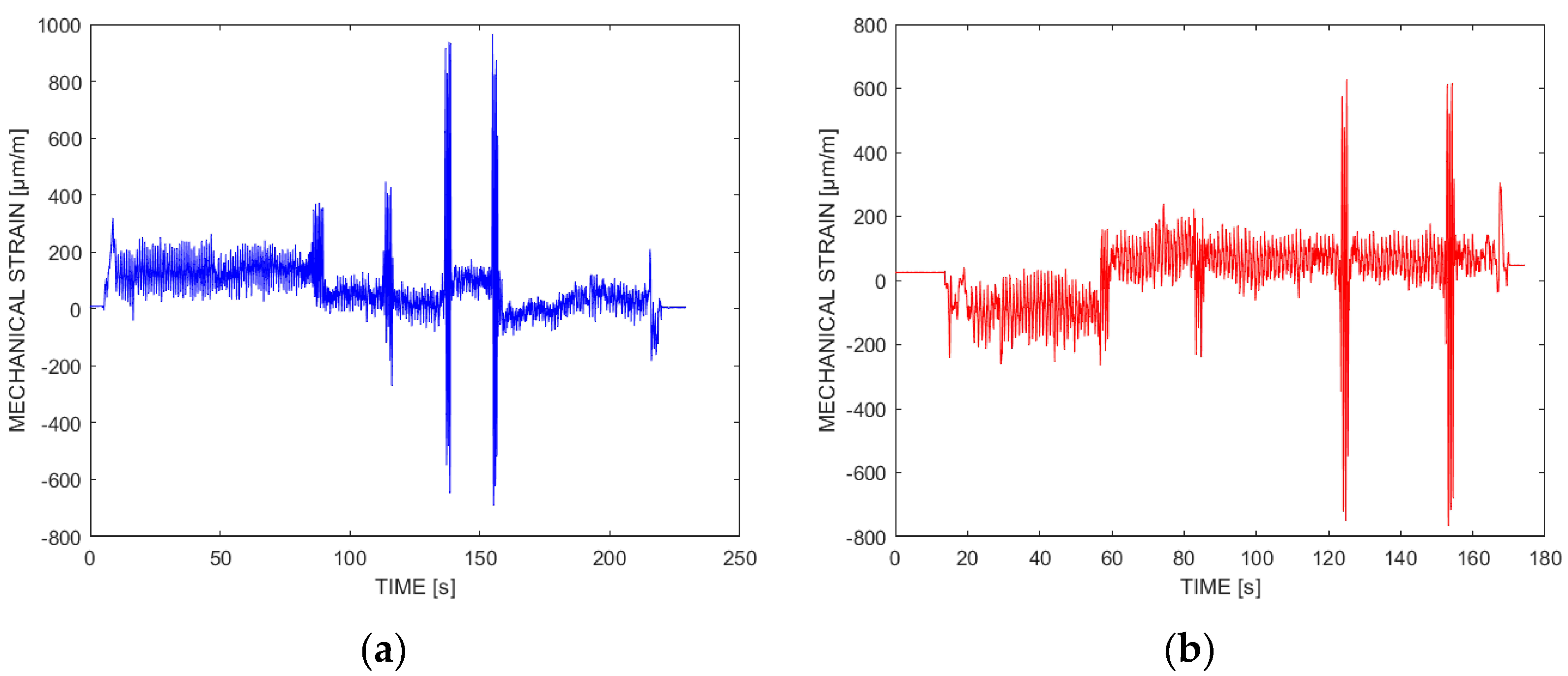
2.6.2. Ergometer Test

The frame was fitted with components and loaded by pedal forces on an ergometer. The ergometer is an exercise machine that loads the rear wheel and creates pedaling resistance. The rider performed a series of sprints in order to obtain the maximum load from pedaling (Figure 8f).

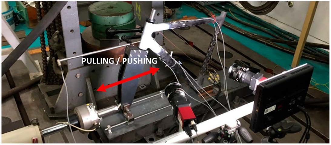
2.6.3. Frame Structural Strength Tests

The experimental work was focused on the most critical load case in terms of rider safety: the horizontal loading force test. The force acting on the fork during a jump, riding over a pothole or a frontal impact was simulated using a hydraulic actuator. Specimens 1, 2, 4, 5, 6 and 7 were tested; Specimens 1, 2, 4 and 7 were loaded by a pushing load, while specimens 5 and 6 were loaded by a pulling load. The experimental set-up and an example of the DIC method evaluation is in Figure 9. The test frame was assembled into the test bed and loaded with an IST PL63 servo-hydraulic actuator with an integrated displacement sensor and a load cell with a range of 63 kN. The position control was used and the loading speed was 8 mm/min. The measurement procedure was terminated when a complete joint failure was achieved. So-called gauge strain values, along the line representing the FBG sensor inside the UD carbon tape from the DIC method, were obtained for the pushing load case using Istra 4D software.

3. Experimental Results and Discussion

First, a tensile test of the UD carbon tape was performed to evaluate the limit of its mechanical strain value. This is an important value, because the UD tape connects the individual tubes of the frame, and if it breaks, the respective joint will collapse. Specimens of the hand-laminated UD tapes and 3k fabric were made and tested to determine the mechanical properties of the joint lamination components. A limit for mechanical strains of 4860 μm/m and 4946 μm/m at breaking point were found for two samples of the UD tapes.

3.1. Standardized Load Cases Results

The mechanical strain of the lower and upper UD carbon tapes was indicated by the embedded FBG sensors, FBG DT and FBG TT. Two strain values were determined from the measured data. The absolute maximum strain value was determined as the maximum of the strain-time record for each standard load case. Furthermore, the maximum strain value from the steady part of the strain-time record (operational maximum deformation) was evaluated, as required by the ISO standard case. This value is decisive in evaluating the frame according to this test and can be found in Table 2 The characteristics of the strain-time record were of two types:
  • Cyclic loading with load control for about 1000 cycles (pedal forces test, horizontal forces test, vertical forces test);
  • Quasi-static loading with a constant load for 3 cycles (bottom bracket stiffness test, head tube torsion stiffness test).
A characteristic record of the first type is shown in Figure 10 for the pedal forces test. Figure 11 is an example of a characteristic record of the second type for the head tube torsion stiffness test.
The maximum strain value from the steady part of the strain-time record (operational maximum deformation) on the surface of the frame tubes in the DTF34 and TTF34 locations (see Figure 4a) was evaluated from the strain gauge’s signals. These values expand the information about the head tube joint area’s mechanical behavior, providing a comparison of the local mechanical strain inside the joint with the mechanical strain measured in its vicinity, on the surface of the tube by the strain gauge. Strain values can be found in Table 2 (marked as SG DTF34 and SG TTF34).
Figure 10 and Figure 12 display the results from the pedal forces test. Maximum indicated strain values of 580 µm/m for FBG DT and −480 µm/m for FBG TT were found. A small asymmetry of the frame is evident, caused by different stiffnesses of the DT and the TT and load distribution in the frame. The indicated strain is greater on the lower down tube, which transmits a larger part of the loading. Deformation in the joints can be considered as significant. At the same time, deformation values of 388 µm/m for SG DTF34 and −364 µm/m for SG TTF34 were measured by the strain gauges. It is obvious that during cyclic loading there is no redistribution of deformations, which could signal the degradation of joint stiffness.
The results of the horizontal forces test also show that in this loading case there is no significant redistribution of deformations or degradation of joint stiffness. For the pushing load direction, the maximal strain value indicated by FBG DT is −210 µm/m and 80 µm/m for FBG TT. The deformations measured by the FBG sensors in the head tube joint are lower here than in the previous case, but are still not negligible. Deformation values of −7 µm/m for SG DTF34 and 5 µm/m for SG TTF34 were measured by the strain gauges.
In the case of the vertical force test, the frame is loaded significantly less and a greater load is transmitted by the seat and upper frame tube in the rear frame section. This is confirmed by the strain values indicated by the FBG sensors inside the UD tapes: concretely, −15 µm/m for FBG DT and −11 µm/m for FBG TT. At the same time, deformation values of 1 µm/m for SG DTF34 and 4 µm/m for SG TTF34 were measured by the strain gauges. Although the time changes during loading are more pronounced than in previous load cases, they are also insignificant on a relative scale.
When testing the bottom bracket stiffness, the load is introduced by means of a weight-defined constant load. Measured strain values of −371 µm/m for FBG DT and 402 µm/m for FBG TT are significant for the head tube joints’ area loading. Strain values of −376 µm/m for SG DTF34 and 375 µm/m for SG TTF34 strain gauges were indicated.
The last of the standardized load cases is the head tube torsion stiffness test (Figure 11). This test measures the torsional rigidity of the frame between the front and rear wheels, which mainly affects the stability of the bicycle at high speeds. The constant load applied to the frame by means of an equivalent test fork induces a considerable load on the head tube, as is evident from the values measured by the FBG sensors. A mechanical strain of −267 µm/m was indicated by FBG DT, while FBG TT read 209 µm/m. Strain values of −117 µm/m for SG DTF34 and 117 µm/m for SG TT34 strain gauges were indicated.

3.2. Ergometer Test Results

After the tests in the laboratory, the frame was fitted with components and loaded by a cyclist on an ergometer. The strain-time series of the test is shown in Figure 13. Deformation of the head tube joints during the two short sprints was greater than during the aforementioned standardized laboratory load case. A maximum indicated strain of 963 µm/m for FBG DT and −743 µm/m for FBG TT was found. This represents an increase in the minimum deformation that the frame must be able to withstand, by 66% in the case of the DT and by 55% in the case of the TT. Strain values of 448 µm/m for SG DTF34 and −262 µm/m for SG TT34 strain gauges were indicated.

3.3. Structural Strength Test Results

The performed ISO standardized tests, which were extended by means of pedaling tests on an ergometer, show that the joints of individual tubes are, from a load transfer point of view, more critical parts of the frame than the tubes themselves. It was shown that the strain values indicated by the embedded FBG sensors, especially in the case of pedal or horizontal loading, are significantly higher than the strain values indicated by the strain gauges. The test program for determining the structural strength of a simplified bicycle frame was therefore focused on a more detailed analysis of the head tube joints. This was achieved by the use of additional strain gauges, digital image correlation and acoustic emission methods.

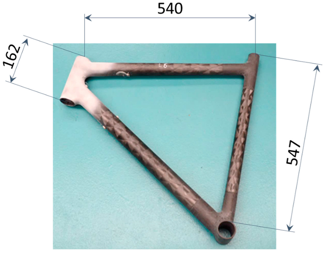
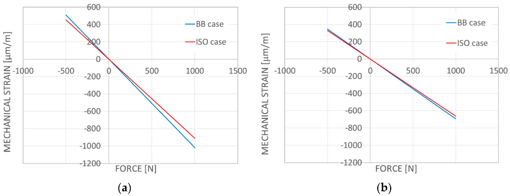
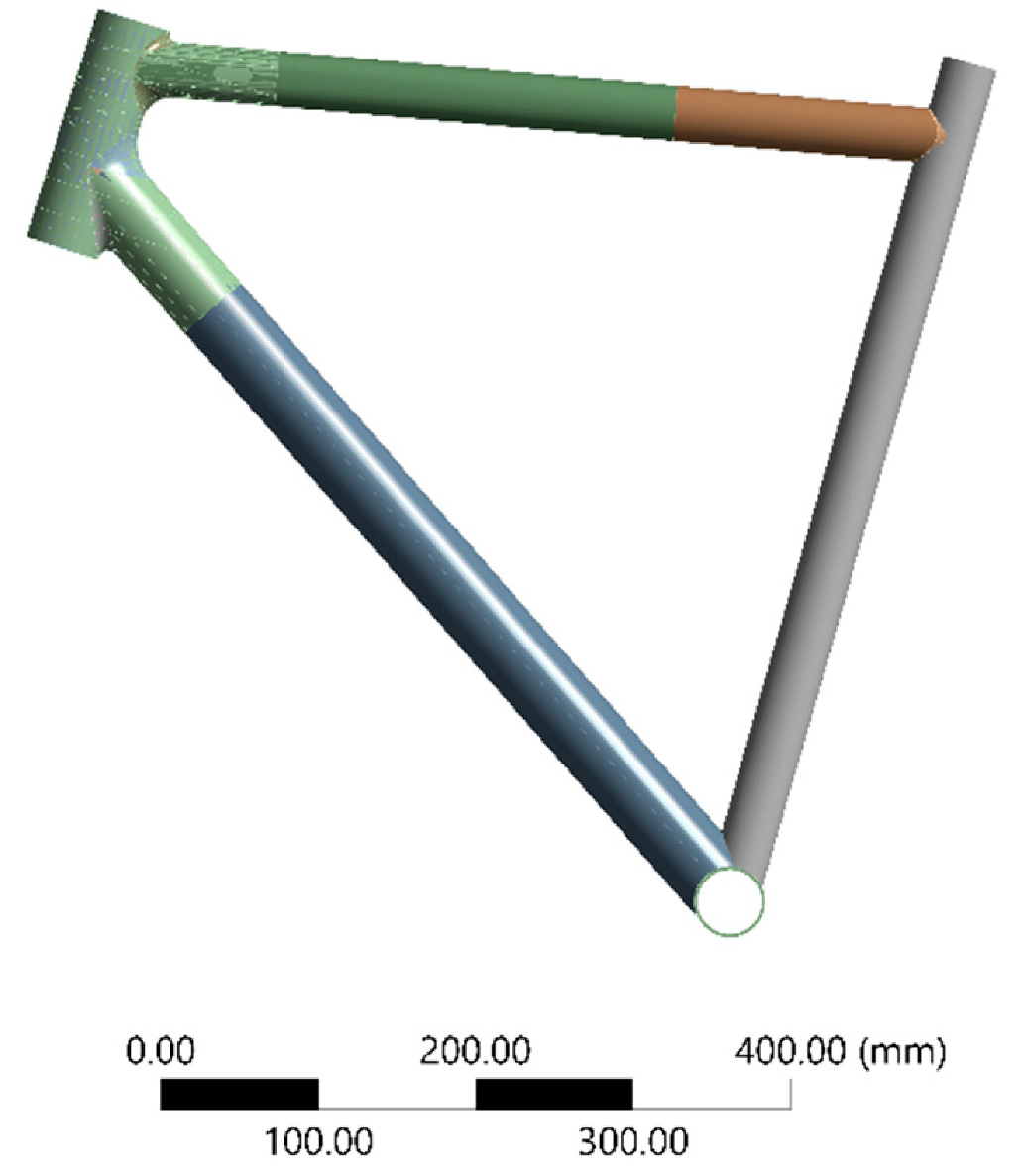
3.3.1. Influence of Frame Simplification

In the first step, the influence of frame simplification from frame specimen 0 to a simple triangle in the case of frame specimens 1, 2, 4, 5, 6 and 7 was evaluated. The question was whether the standard ISO case (specimen 0), where the frame is attached to the ground using rear dropouts, was equivalent to the simplified case, where the frame is attached using the bottom bracket tube (BB case, specimens 1, 2, 4, 5, 6 and 7). For both cases, the loading using the equivalent test fork was identical. Strain gauges were installed on all the tested frames near the head tube (DTF1, 2 and TTF1, 2 in Figure 4). These strain gauges were placed on the top and bottom surfaces of the tubes and connected using the quarter-bridge measurement scheme, from which the bending strain component was calculated. The dependence of the measured mechanical strain on the loading force of the fork is plotted in Figure 14a for the DTF location and in Figure 14b for the TTF location. A linear flexibility response of the frame was found, with values of −0.91 μm/m/N compared to −1.02 μm/m/N (12% increase) at the DTF location. At the TTF location, values of −0.66 μm/m/N and −0.69 μm/m/N were found (an increase of 4.8%). This corresponds to the supposedly increased portion of load transfer by the simplified frame triangle, while the DT transfers a bigger part of the load. The simplification of the load case scenario from the mounting by using the rear dropouts to the mounting, which is using the bottom bracket, is viable. The upper and lower frame tubes are strained slightly more; however this is still on the safe side.

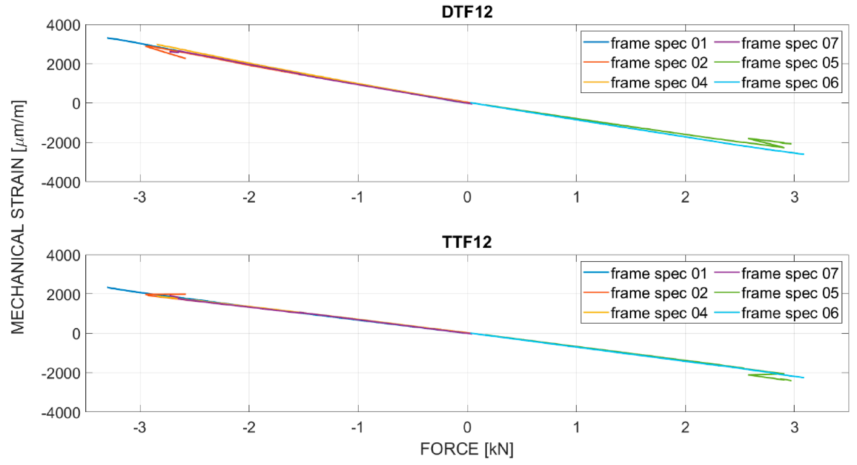
3.3.2. Simplified Frame Structural Strength Testing

As mentioned in the above text, bicycle frame specimens 1, 2, 4, 5, 6 and 7 were tested until their final failure; specimens 1, 2, 4 and 7 were loaded by a pushing load, while specimens 5 and 6 were loaded by a pulling load. The experimental configuration is shown in Figure 9. The maximum force at failure was indicated when the first peak maximum was reached. A range of forces from −3.3 kN to 3.1 kN was found. Load curves for both pushing and pulling cases are shown in Figure 15. A linear dependence in the response of the strain gauge installed on the TT and the DT frame tubes near the head tube (DTF12 and TTF12, see Figure 4a) can be seen over the entire range, from zero force to the maximal indicated force.
To compare the strain measurement methods, the average longitudinal strain was evaluated (using the DIC method) along the line representing FBG sensor routing in its sensing area. This was performed for frame specimens 1, 2, 4 and 7 (pushing load case). The maximum value of the strain was deducted at the moment when the maximum loading force for a specific frame specimen was reached. The resulting values of the limit of the mechanical strain for Fmax are shown in Table 2.

3.3.3. Summary of Experimental Results for the FBG Sensors

A summary of the results of the experimental analysis performed on the composite bicycle frame using the FBG sensors and strain gauges is shown in Table 2. It is obvious that when testing on the ergometer, higher values of the indicated deformations were achieved than in any of the cases defined in the ISO test standard.
If we compare the corresponding load cases, i.e., the horizontal forces test case and the frame structural strength test (both for a pushing load case direction), the indicated values of mechanical strain in the DT and HT joint area are at the level of 10–13% of the maximum strain value, while in the case of the TT and HT joint it is 5–7%.
The ultimate mechanical strain measured at the TT and HT joint reaches 35% of the ultimate mechanical strain found during the tensile strength test of unidirectional filaments ud1 and ud2. This means that these reinforcing strips are not a limiting element of the joints of individual tubes in the case of tensile strain.
The highest and lowest values of mechanical strain, measured by FBG sensors in ISO test cases (580 μm/m for FBG DT, −480 μm/m for FBG TT), are in the range of 27–37% and 28–44% of the limit mechanical strain found during the frame structural strength test at the point of FBG DT and at the point of FBG TT, respectively.
The highest and lowest values of mechanical strain, measured by FBG sensors during the ergometer test (963 μm/m for FBG DT, −743 μm/m for FBG TT), are in the range of 45–61% and 44–68% of the limit mechanical strain found during the frame structural strength test at the point of FBG DT and at the point of FBG TT, respectively.
If we compare the mechanical strain values from the FBG sensors (in the FBG DT and FBG TT locations) and the values from the strain gauges (in the SG DTF34 and SG TT34 locations), the stresses inside the DT to HT and the TT to HT joints are higher than on the frame tubes. This is especially true for load cases corresponding to the normal operation of the bike frame, i.e., the pedal forces test case, horizontal forces test case and the ergometer test. Other experimental and computational work therefore focused in more detail on the head tube joint.

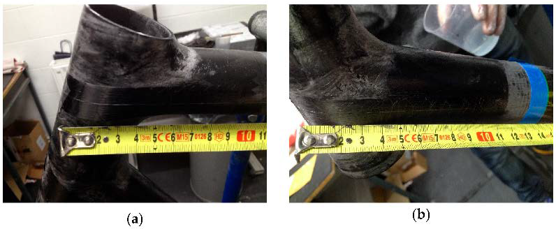
3.3.4. Influence of Head Tube Joint Reinforcement

During the structural strength test of the frame, attention was also focused on evaluating the effect of reinforcing the composite lay-up of the head tube joint by adding both unidirectional carbon filament layers and carbon fabric layers. For this purpose, strain gauges were installed on the rear side of the head tube (location HT, see Figure 5a). This location was chosen because there is the same composite lay-up for all frame specimen designs. The mechanical strain measured by the strain gauge at the HT location on the head tube, depending on the loading force, is plotted in Figure 16 for specimen 4 with the original composite lay-up and for specimen 7 with the reinforced composite lay-up. In the case of frame specimen 7, there was a delay in the loading process at about 2.3 kN due to technical reasons. We can see that the load characteristic indicated by the HT4 strain gauge on frame specimen 4 is linear up to a load of approximately 1 kN, with Fmax reaching 2.85 kN. In the case of frame specimen 7, the load characteristic indicated by the HT7 strain gauge shows a linear response up to approximately 1.3 kN, while the Fmax of 2.82 kN was reached. According to the strain gauge at the HT location, frame specimen 7 behaves better than frame specimen 4 in terms of the operational properties of the bike. The loss of linear response occurs at about 35% of the limit load in the case of specimen 4, while in the case of specimen 7, this occurs later, at about 46% of the limit load due to the reinforcement of the head tube joint area.
The DIC method was used to find the extreme strain values in the head tube joint area. A comparison of the identified behaviors of the two selected specimens in the head tube joint area for the step just before failure is shown in Figure 17a (frame specimen 4) and Figure 17b (frame specimen 7). In comparing these two specimens with a specified field of the principal strain 1, it can be seen that specimen 4 is characterized by higher strain values near the TT to the HT joint, located with the maximum on the top side. The strain values around the joint of the DT to the TT are not as high, which is in accordance with the final failure which first appeared in the TT to the HT joint part of the specimen, while the DT to the HT joint remained almost undamaged. On the contrary, the strain values for specimen 7 are high in both joint areas, which correlates again with the final failure of both joints at the same time. Reinforcement of the joints that were made for specimen 7 apparently leads to a more balanced distribution of loading between joints.
The mean values over the area of principal strain 1 were evaluated in three sections (as described in Section 2.4). The values of the down tube for specimen 4 (Figure 18a) and specimen 7 (Figure 18b) were compared. Based on these comparisons, it can be seen that both specimens are equally stiff on the selected sections. Strengthening of joints for specimen 7 clearly helped in the DT to the HT joint area, whereas specimen 4 shows the appearance of a local failure in the G1 area (using the sensor marking described in Figure 6). The indicated local failure corresponds to a slight decrease of force (shortly after reaching time step no. 500) and also to a slight strain increase in the G2 area. The failure detected in this area also correlates with an increase of counts shown by the AE method in the same time period (boxtime value around 5.324 × 10⁴ s.). A force signal measured in specimen 7 also indicates a slight decrease of force during loading (step value around no. 230), but there were no failures indicated in the gauge areas.
Due to the fact that the growth of the damage in the initial phase has only a local effect on the strain distribution and does not significantly affect the global stiffness response of the frame, as indicated by the loading force and the displacement measured by a hydraulic actuator, the acoustic emission method was used. The three sensors were installed on individual tubes according to Figure 7. The recorded acoustic events are plotted together with the loading force in Figure 19 (frame specimen 4) and in Figure 20 (frame specimen 7). From the results of the AE method in the case of frame specimen 4, it is evident that the AE events count begins to increase when a load force of 1.34 kN is reached, while in the case of frame specimen 7 this occurs when 1.60 kN is reached. Another fact evident from the comparison of the graphs is the different behavior of the AE sensors located on the TT in the E1 location and on the DT in the E3 location. In the case of frame specimen 4, more acoustic events were indicated at the E1 location, indicating head tube to top tube joint cracking, while at E2, the rate of AE event acquisition was slower. In the case of frame specimen 7, the rate of increase of the AE event count at locations E1 and E3 is similar.
The graph for frame specimen 7 also shows that the load stops when it reaches about 2.35 kN and then the loading force is maintained at a constant level, while no increase in the AE event count is indicated. This means that even when damaged up to this level, the stress in the undamaged frame parts is not high enough for this force to cause stress redistribution, resulting in further overloading of the frame and further damage.
This confirms that through the optimization and strengthening of the head tube joint area, both a higher load-bearing capacity of the frame and a better stress distribution in the DT and TT to HT connections were achieved.

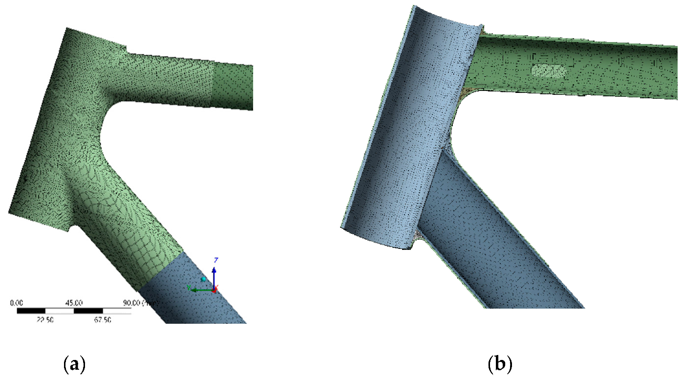
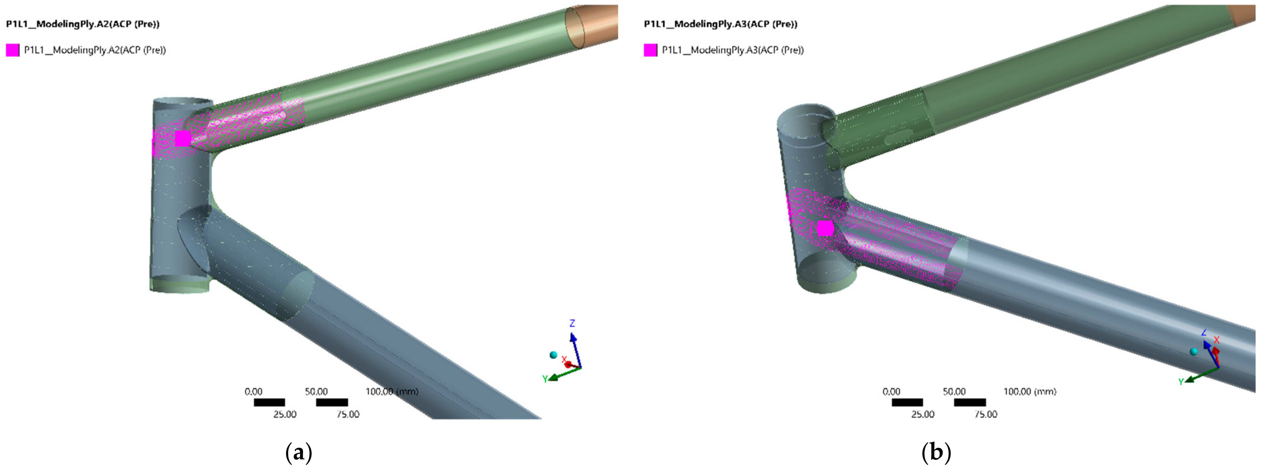
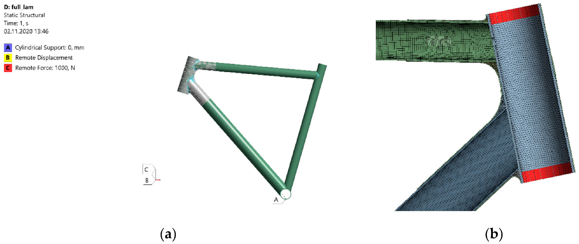
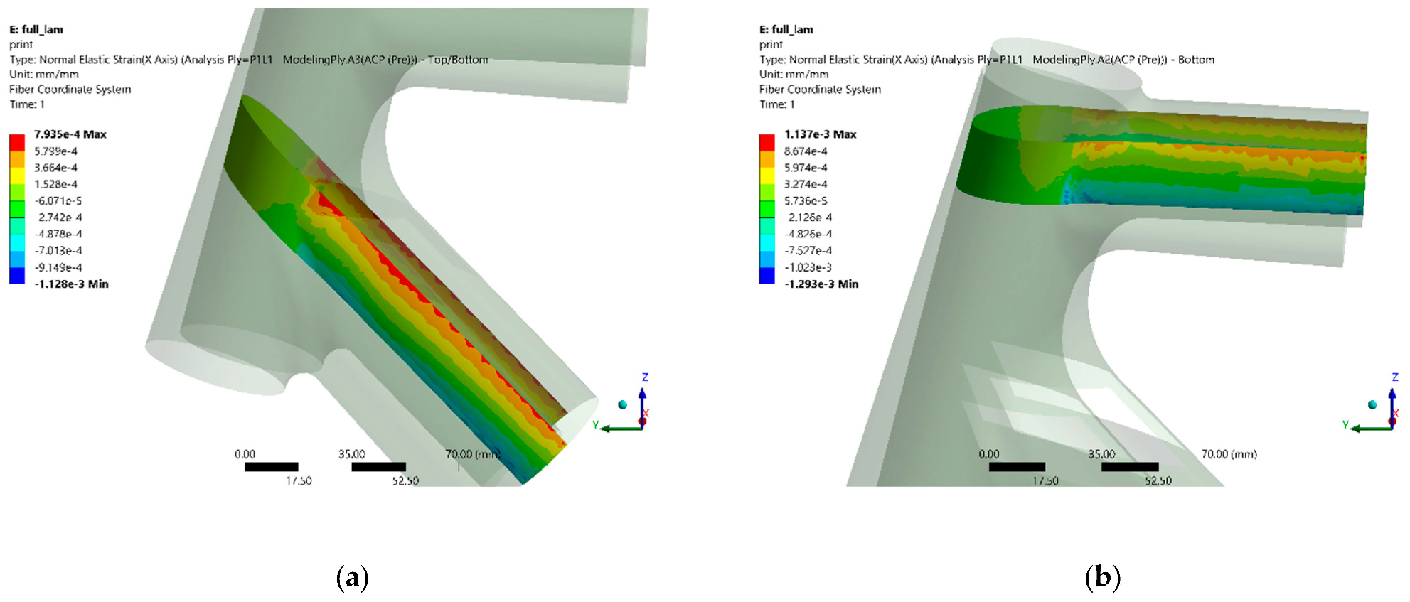
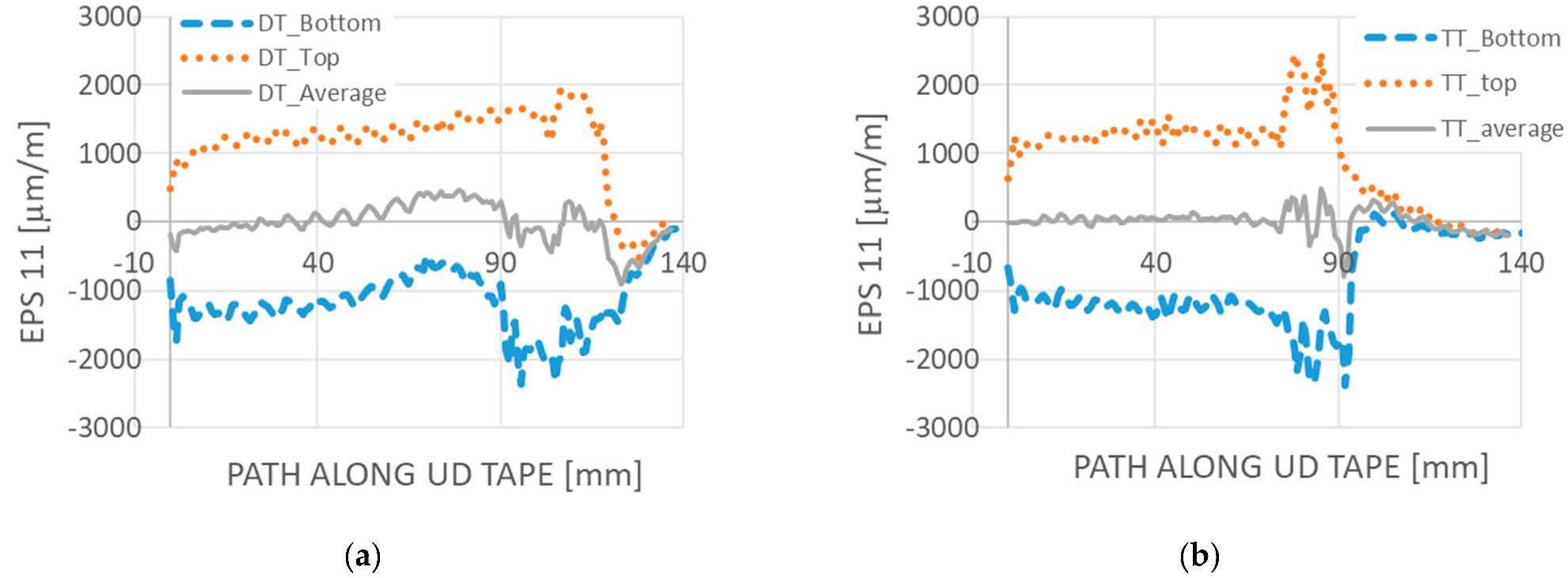
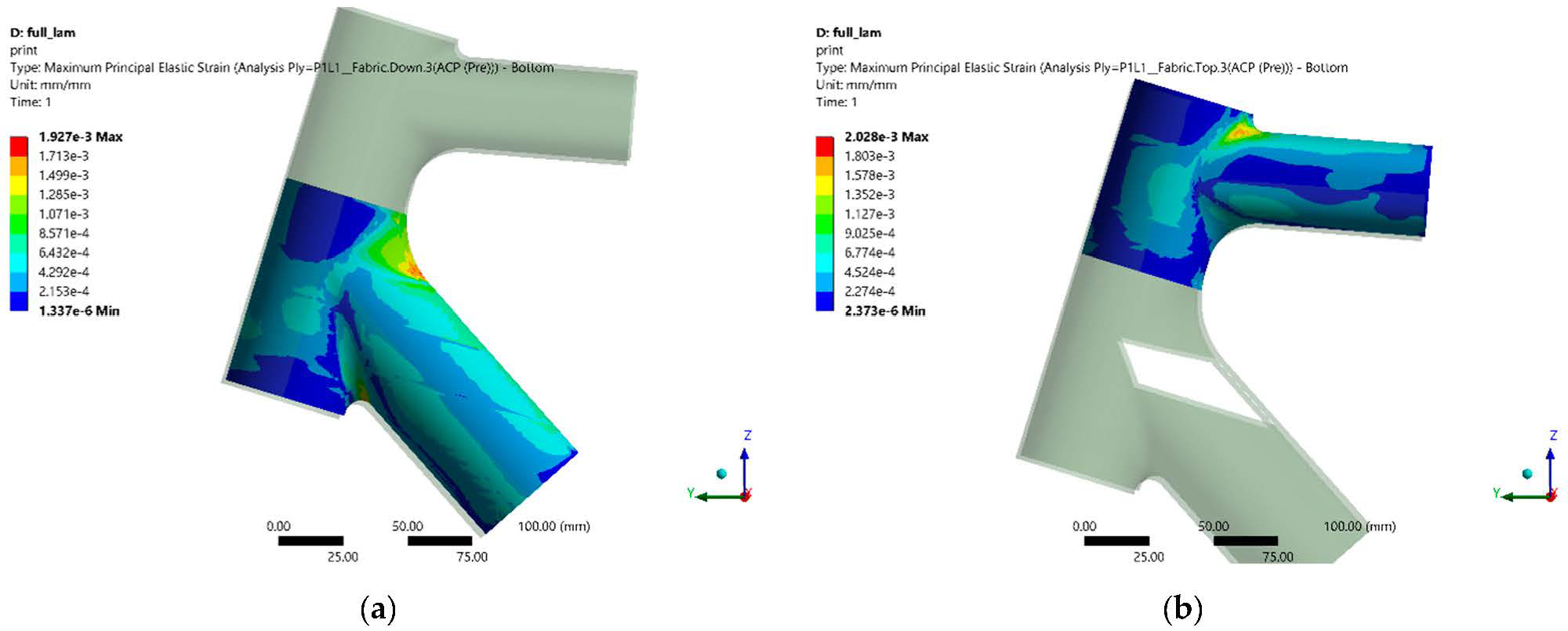
3.4. Finite Element Method and Results

The application of FBG sensors into the joint area is further complicated by the stress distribution in the laminated joint. A finite element (FE) analysis of the simplified frame during the structural strength testing was performed. The FE model (see Figure 21) consists of the main structural tubes (head tube, down tube, top tube, seat stay) together with the model of the head tube—down tube—top tube joint. The rest of the frame was not modelled as the aim was to compare the loading in the head tube joint area; the rear part of the frame was assumed to not influence the behavior and was omitted from the model.
The simulation was performed in ANSYS Mechanical 2021 R1 (ANSYS, Inc., Southpointe 2600 Ansys Drive, Canonsburg, PA, USA) software using ANSYS Composite Prepost for the definition of the shell parameters in the joint area. The structural tubes were modelled using solid-shell elements with one solid-like element per wall thickness; every layer of the lay-up was specified to define the tube’s behavior. The joint area consists of three composite structural tubes, foam fillers and the composite lamination, as shown in Figure 22. The solid-shell elements of the structural tubes were of size 1.8 mm, the quadratic tetrahedron elements of the foam filler were of size 1.0 mm and the conventional shell elements of the lamination were of size 0.8 mm. The components were connected using “MPC bonded” contact options. The following material properties were used for UMS40: Ex = 210,666 MPa, Ey = Ez = 4921 MPa, Gxy = Gyz = Gxz = 3286 MPa, and for T700: Ex = 137,476 MPa, Ey = Ez = 5300 MPa, Gxy = Gyz = Gxz = 3648 MPa.
The joint lamination consists of UD tapes and fabric layers, which were placed over the tubes and foam fillers. The whole lamination was modelled using one conventional shell element per wall thickness. The composite prepost toolkit was used to specify the correct sequence of layers, together with each layer wall thickness and fiber orientation. An example is shown in Figure 23, where the UD type from the top tube to the head tube and UD tape from the down tube to the head tube is shown. These tapes were used to evaluate the deformation of the model for the specified loading and to compare the results with the FBG sensors.
The linear static analysis was performed with the focus on evaluating the deformation of the frame in the joint area and the deformation of the lamination of the two UD tapes, which corresponded to the location of the FBG sensors. The boundary conditions were derived from the experimental measurement (see Figure 24). A cylindrical support was used in the BB tube; the force was applied to the remote point in the position taken from the experiment. The loading point was connected to the areas where the bearings between the loading fork and head tube were placed (see highlighted areas in Figure 24b). The loading point DOFs were constrained to only allow motion in the direction of the acting force.
The FBG sensors were integrated into one UD tape, which connected the down tube with the head tube, and into the UD tape, which connected the top tube with the head tube. The position of the sensors is highlighted in Figure 6a.
For the aforementioned tapes with integrated FBG sensors, the strain distribution along the UD tape is displayed in Figure 25, using the FE simulation of the structural frame test for a nominal loading. Coordinate 0 of the path was at the beginning of the UD tape, while coordinate 140 mm corresponds approximately to the position of the tape at the middle of the head tube. The strain component along the fiber direction was selected as the analyzed parameter. The FE analysis values were obtained from the top and bottom edge of the tape and the strain values in the FBG sensor position were averaged from both edges, as the sensors were placed approximately in the middle of the UD tape. The positions of the FBG sensors were approximately at coordinate 111 mm for the DT and 99 mm for the TT (see Figure 26).
The strain distribution for the specified loading case clearly demonstrates that the positioning of the FBG in the tape is crucial for the reading and evaluation of the data. Depending on the positioning in the tape, the loading can be either in tension or compression, if the sensor is placed close to the edges of the most important UD tapes of the joint lamination.
The maximum principal elastic strain evaluated on the surface of the head tube joint is shown in Figure 27a for the DT to HT connection and in Figure 27b for the TT to HT connection area. From the comparison with Figure 17, it can be seen that the character of the principal strain 1 distribution on the surface of the joint area is similar, with the compressive deformation of the bottom of the DT and the tensile deformation of the top of the DT. Likewise, in the case of the TT, the top of the tube is stretched and the bottom of the tube is compressed. However, from the result of the FEA performed on the UD tape, it is obvious that the tape is loaded by bending on the surface of the joint. When viewed from the side, the tensile strain can be seen; however, the strain distribution is very uneven. Thus, as in the case of an embedded FBG sensor, when the measured strain depends on the position of the FBG sensor inside the UD tape, the strain gauge measurement on the joint surface would also be difficult due to the result of the measured strain, which is highly dependent on the strain gauge position, size and orientation to the composite layer axes. In addition, the characteristic of the layered composite is applied in the joint with a 3D complex geometry, where in addition to the magnitude of the deformation, the direction of the indicated strain also differs in the individual layers of the lay-up. This makes classical strain analysis difficult. In the case of the FBG sensors, which were embedded into the only place where it was technologically possible, i.e., between the layers of the UD tape and its neutral axis, the sensitivity to the position of the sensor is large. However, a relative comparison of individual load cases is possible.

4. Conclusions

Extensive experimental research into the behavior of a composite bicycle frame was performed with a focus on the manually laminated tube-to-tube connection of the frame’s down tube with the head tube, and of the top tube to the head tube.
The first part of this research focused on the bicycle frame‘s behavior during the mandatory ISO test load cases, which are necessary in order to approve such frames for commercial use. Using FBG sensors embedded inside the UD load bearing tapes in the HT joint area, the envelope of the required minimal operational strain range was identified. Monitoring the rider’s safety, critical strain values were found, especially for loads simulated by sprinting on the ergometer, detecting an increase of up to 66% above the values resulting from the required ISO-defined standard tests. This clearly demonstrates the importance of, at the very least, a basic operational strain analysis of such a structure, which is optimized for a combination of strength, stiffness and weight. The highest absolute strain found by the FBG sensors in this analysis corresponded to 68% of the HT joint limit strain found during the frame structural strength test. The safety of the composite frame is therefore sufficient; however, further development of the frame structure would require a complete field operational strain measurement. A comparison of the responses from strain gauges installed on the surfaces of the tubes near the HT joints with the responses of embedded FBG sensors in the HT joint when testing load cases corresponding to standard frame use, such as a pedal forces test or a horizontal forces test, was performed. It showed that, regarding load transfer, HT joints are critical and that further development of the frame must focus on their improvement. Furthermore, it was found that under cyclic loading, there is no redistribution of deformations that could signal the degradation of the HT joints’ stiffness.
The second follow-up part of this research was carried out on simplified frame specimens without chains and seat stays. Both resistive strain gauges for local analysis and the DIC method for obtaining the strain field were used, supplemented by the AE method for the detection of composite defects and the FEA of individual composite joint layers. The aim was a deeper analysis of the deformation of the HT joint and an increase in the strength of the frame in the HT joints.
The performed FEA of the composite lay-up of the HT joint showed a high sensitivity of the methods for local strain analysis, such as strain gauges and FBG sensors, to the position of the particular sensor. From the deformation analysis of the UD tape, it is evident that the FBG sensor can achieve deviations of up to 100% against the position in the neutral axis; moreover, with the opposite sense of strain. However, with a constant sensor position and on one frame specimen, a relative comparison of different types of loads is possible. It can be concluded that the FBG sensors have shown good functionality in the local monitoring of the critical joints of the composite bicycle frame.
The same situation would of course occur when using resistive strain gauges installed on the joint surface. The advantage of methods that do not require prior computational analysis for placing the sensor, such as DIC which can cover the entire test area, is clearly demonstrated.
Using a combination of the DIC method, the HT strain gauge measurement and the AE method, the improvement of frame specimen 7 in terms of strength compared to the frame specimen 4 sample was confirmed. By adding a combination of fabric layers and UD tape to the HT joints, the point when the load characteristic measured by strain gauges stopped being linear had moved from 35% to 46% of the limit load. This confirms a better use of the linear response operating area of the frame. This was also confirmed by the AE method, where the detection of first cracks occurred at 47% (in the case of frame specimen 4) and 57% (in the case of frame specimen 7) of the limit load. The AE method also made it possible to identify which of the HT connections was broken first. An improvement in the frame strength properties was also found using the DIC method, when comparing the indicated mechanical deformation evaluated for three places on the DT. It can be seen that in the case of frame specimen 7, there were no sudden changes in the indicated strain (which would mean cracking in the joint) to the maximum forces at failure.

Author Contributions

Writing—original draft preparation, M.D. and V.K.; bicycle frame with embedded sensors manufacturing, M.D., T.P. and N.S.; experimental work, M.D., K.D., M.R. and T.P.; FBG data analysis, M.D. and T.P.; AE and DIC data analysis, B.K. and M.D. All authors have read and agreed to the published version of the manuscript.

Funding

This work was supported by the Technology Agency of the Czech Republic within Programme for funding of applied research ZETA, through project “Development of integrated joints of composite profiles”, project no. TJ02000252.

Institutional Review Board Statement

Not applicable.

Informed Consent Statement

Not applicable.

Data Availability Statement

Data sharing is not applicable to this article.

Acknowledgments

The authors would like to thank Festka s.r.o. for material, technical and experimental support.

Conflicts of Interest

The authors declare no conflict of interest.

Appendix A

Appendix A.1. Fiber Bragg Grating Sensors

The FBG sensor is an intrinsic spectrometric type of sensor, which has been intensively developed since its invention in the early 1990s [23]. It is based on a periodic variation in the refractive index of the fiber core, which reflects particular wavelengths of light and transmits all the other wavelengths. The FBG sensor’s working principle is based on a sensitivity to changes in strain and temperature of the grating period and refractive index. Each Bragg grating is characterized by a so-called Bragg wavelength, which shifts according to the deformation of grating [24,25].
In practice, there are two methods of manufacturing Bragg gratings for sensing purposes (FBG sensor) [26]. The standard procedure is to remove the primary coating (usually polyacrylate) from a common telecommunication optical fiber. The grating is then made using a UV laser and phase mask. The fiber is recoated to restore its protection. The resulting sensor has a maximum elongation at a break of about 1% and reflectivity up to 99% [27,28]. FBG sensors with a higher possible elongation (up to 7% [21,29], coated by polyimide or ORMOCER®) are produced by the combined process of a simultaneous drawing of the fiber and a writing of the grating. Because the inscription to the core is made through the primary coating and the energy of the laser is low, the final FBG sensor has a lower reflectivity (up to about 30%) but better mechanical properties. A tensile strength at a break of up to 50 N with an elongation of about 5% were determined experimentally in [30].
Table A1. FBG sensor and measurement device properties [21,22].
FBG Sensor PropertiesSafibra FBGuard Measurement Device Properties
Grating length8 mmWavelength range1505–1590 nm
Reflectivity>15%Wavelength resolution≤1 pm
Cladding diameter125 μm ± 1 μmWavelength repeatability±5 pm (max.)
Coating typeORMOCER®Scan frequencyup to 11 kHz
Coating diameter195 μmDynamic range30 dB
Temperature sensitivity6.5 K−1 × 10⁻⁶Optical connectorFC/APC
Strain sensitivity7.8 με−1 × 10⁻⁷Active channels1
Temperature range−200 ÷ 200 °C

Appendix A.2. Resistive Strain Gauges

Resistive strain gauges are a long-used and proven method for measurement. Their working principle is that the strain of the measuring object is transferred to a strain gauge and causes a change to its electrical resistance with linear dependency. A small change of resistance is generally indicated by means of a Wheatstone circuit, when the circuit complementation is part of the strain gauge measurement unit [31].
Table A2. Strain gauge sensor and measurement device properties.
Strain Gauge Sensor PropertiesMeasurement Device Properties
Grid length6 mmChannels8
Resistance350 Ω ± 0.35 %Carrier frequency600 Hz
Transverse sensitivity0.3 %Transducer exc. voltage2.5 V
k—Gauge factor2.04 ± 1.0 %TransducersSG, DC
Temperature range−200 ÷ 200 °CAccuracy class0.1

Appendix A.3. Digital Image Correlation

The 3D digital image correlation method (DIC) was used to identify the surface strain field in the head tube area. DIC is a non-contact optical method allowing material points to be tracked during a deformation (e.g., see [32] for detailed information about the method). First, a random surface pattern is created. An evaluation algorithm identifies the material points in gray-scaled consecutive images of a specimen. Finally, a displacement is found where the mapping between consecutive images results in the highest correlation. Measured displacement patterns could be used to calculate strain during evaluation. The DIC method could be arranged in a 2D or 3D arrangement, allowing an in-plane or even out-of-plane measurement of displacements.

Appendix A.4. Acoustic Emission Method

The acoustic emission method (AE) is a non-destructive method of monitoring specimen damage. The working principle is to detect the elastic stress wavefronts which are propagated in a component, generated by the dynamic release of mechanical stress inside the material body—acoustic emission events [33]. These events occur with the displacements of dislocations, dynamic micro-crack formations, etc., and propagate in the specimen as both dilatation and shear waves. These waves are detected by the piezoelectric AE sensors. They are then converted from the mechanical deformation to the corresponding electrical signal, which needs to be amplified, transmitted, processed and stored by the measuring device. The amplification of the detected signal is an important factor that prevents possible interference of the signal being measured. This can be caused by the influence of the environment and the transmission of the electrical signal [34].
Table A3. Acoustic emission sensor and measurement device properties.
AE Sensor PropertiesMeasurement Device Properties
Diameter9 mmChannels5
Case materialStainless steelSampling8 M sample/s
Face materialCeramic ø 6 mmDC inputs15
Piezoceramic materialPZT class 200DC outputs16
Temperature range−20 ÷ 90 °C

References

  1. Khosravani, M.R. Composite Materials Manufacturing Processes. Appl. Mech. Mater. 2012, 110–116, 1361–1367. [Google Scholar] [CrossRef]
  2. Akderya, T.; Kemiklioğlu, U.; Sayman, O. Effects of Thermal Ageing and Impact Loading on Tensile Properties of Adhesively Bonded Fibre/Epoxy Composite Joints. Compos. Part B Eng. 2016, 95, 117–122. [Google Scholar] [CrossRef]
  3. Juang, J.-N. Applied System Identification; Prentice Hall: Englewood Cliffs, NJ, USA, 1994; ISBN 978-0-13-079211-2. [Google Scholar]
  4. Farzampour, A.; Kamali-Asl, A.; Hu, J.W. Unsupervised Identification of Arbitrarily-Damped Structures Using Time-Scale Independent Component Analysis: Part I. J Mech Sci Technol 2018, 32, 567–577. [Google Scholar] [CrossRef]
  5. Farzampour, A.; Kamali-Asl, A.; Hu, J.W. Unsupervised Identification of Arbitrarily-Damped Structures Using Time-Scale Independent Component Analysis: Part II. J. Mech. Sci. Technol. 2018, 32, 4413–4422. [Google Scholar] [CrossRef]
  6. Vanwalleghem, J.; De Baere, I.; Loccufier, M.; Van Paepegem, W. Development of a Multi-Directional Rating Test Method for Bicycle Stiffness. Proc. Procedia Eng. 2014, 72, 321–326. [Google Scholar] [CrossRef]
  7. Sisneros, P.M.; Yang, P.; El-Hajjar, R.F. Fatigue and Impact Behaviour of Carbon Fibre Composite Bicycle Forks. Fatigue Fract. Eng. Mater. Struct. 2012, 35, 672–682. [Google Scholar] [CrossRef]
  8. Hoes, M.J.A.J.M.; Binkhorst, R.A.; Smeekes-Kuyl, A.E.M.C.; Vissers, A.C.A. Measurement of Forces Exerted on Pedal and Crank during Work on a Bicycle Ergometer at Different Loads. Int. Z. Angew. Physiol. Einschl. Arbeitsphysiol. 1968, 26, 33–42. [Google Scholar] [CrossRef]
  9. Petrone, N.; Giubilato, F.; Giro, A.; Mutinelli, N. Development of Instrumented Downhill Bicycle Components for Field Data Collection. Procedia Eng. 2012, 34, 514–519. [Google Scholar] [CrossRef]
  10. Hölzel, C.; Hoechtl, F.; Senner, V. Operational Loads on Sport Bicycles for Possible Misuse. Procedia Eng. 2011, 13, 75–80. [Google Scholar] [CrossRef]
  11. Covill, D.; Begg, S.; Elton, E.; Milne, M.; Morris, R.; Katz, T. Parametric Finite Element Analysis of Bicycle Frame Geometries. In Proceedings of the the 2014 conference of the International Sports Engineering Association, Sheffield, UK, 14–17 July 2014; pp. 441–446. [Google Scholar]
  12. Lessard, L.B.; Nemes, J.A.; Lizotte, P.L. Utilization of FEA in the Design of Composite Bicycle Frames. Composites 1995, 26, 72–74. [Google Scholar] [CrossRef]
  13. Liu, T.; Wu, H.-C. Fiber Direction and Stacking Sequence Design for Bicycle Frame Made of Carbon/Epoxy Composite Laminate. Mater. Des. 2010, 31, 1971–1980. [Google Scholar] [CrossRef]
  14. Boller, C.; Chang, F.-K.; Fujino, Y. Encyclopedia of Structural Health Monitoring|Wiley; John Wiley & Sons: Hoboken, NJ, USA, 2009; ISBN 978-0-470-05822-0. [Google Scholar]
  15. Raymond Measures. Structural Monitoring with Fiber Optic Technology, 1st ed.; Academic Press: Cambridge, MA, USA, 2001; ISBN 978-0-08-051804-6. [Google Scholar]
  16. ISO 4210:2015; Cycles—Safety Requirements for Bicycles. International Organization for Standardization: Geneva, Switzerland, 2015.
  17. EN ISO 4210-6:2015; Cycles—Safety Requirements for Bicycles—Part 6: Frame and Fork Test Methods. International Organization for Standardization: Geneva, Switzerland, 2015.
  18. ISO 4210-2:2015; Cycles—Safety Requirements for Bicycles — Part 2: Requirements for city and trekking, young adult, mountain and racing bicycles. International Organization for Standardization: Geneva, Switzerland, 2015.
  19. Clarification Guide of the UCI Technical Regulation. Available online: https://www.uci.org/docs/default-source/equipment/clarificationguideoftheucitechnicalregulation-2018-05-02-eng_english.pdf?sfvrsn=fd56e265_70 (accessed on 10 August 2019).
  20. The ISO 4210 Standard for Bike Tests Sets a Floor, not a Ceiling. Available online: https://www.zedler.de/en/zedler-aktuell/publikationen/news-detail/the-iso-4210-standard-for-bike-tests-sets-a-floor-not-a-ceiling.html (accessed on 10 August 2019).
  21. DTG® & FSG® Technology. Available online: https://fbgs.com/technology/dtg-fsg-technology/ (accessed on 23 November 2020).
  22. FBGuard—Advanced Monitoring System. Available online: http://www.safibra.cz/download.php?group=stranky3_soubory&id=225 (accessed on 20 November 2020).
  23. Balageas, D.; Fritzen, C.-P.; Güemes, A. Structural Health Monitoring|Wiley; Wiley-ISTE: London, UK, 2006; ISBN 978-1-905209-01-9. [Google Scholar]
  24. Ruzicka, M.; Dvorak, M.; Doubrava, K. Strain Measurement with the Fiber Bragg Grating Optical Sensors. In Proceedings of the 50th Annual Conference on Experimental Stress Analysis, Tabor, Czech Republic, 4–7 June 2012; pp. 385–392. [Google Scholar]
  25. Shizhuo, Y.; Ruffin, P.B.; Francis, T.S. (Eds.) Fiber Optic Sensors; CRC Press: Boca Raton, FL, USA, 2008; ISBN 978-0-367-38756-3. [Google Scholar]
  26. Kreuzer, M. Strain Measurement with Fiber Bragg Grating Sensors. Available online: http://www-personal.umich.edu/~bkerkez/courses/cee575/Handouts/7FBGS_StrainMeasurement_mo.pdf (accessed on 20 November 2020).
  27. SmartFBG Fibre Bragg Grating Sensor. Available online: https://www.smartfibres.com/files/pdf/SmartFBG.pdf (accessed on 23 November 2020).
  28. Preliminary Data Sheet—FBG Sensor Chain. Available online: https://fisens.com/wp-content/uploads/2019/07/2019-06-21-FBG-Sensor-Chain-datasheet.pdf (accessed on 24 November 2020).
  29. DTG coating Ormocer®-T for Temperature Sensing Applications. Available online: https://fbgs.com/wp-content/uploads/2019/03/Introducing_and_evaluating_Ormocer-T_for_temperature_sensing_applications.pdf (accessed on 23 November 2020).
  30. Dvořák, M.; Růžička, M.; Horný, L.; Kábrt, M. The Use of FBG Sensors for Monitoring of the Composite Wing Structure. In Proceedings of the 11th European Conference on NDT Proceedings, Prague, Czech Republic, 6–10 October 2014. [Google Scholar]
  31. Hoffmann, K. An Introduction to Measurements Using Strain Gages; Hottinger Baldwin Messtechnik GmbH: Darmstadt, Germany, 1989. [Google Scholar]
  32. Sutton, M.A.; Orteu, J.J.; Schreier, H. Image Correlation for Shape, Motion and Deformation Measurements: Basic Concepts, Theory and Applications; Springer: New York, NY, USA, 2009; ISBN 978-0-387-78746-6. [Google Scholar]
  33. EN 1330-9:2017; Non-Destructive Testing—Terminology—Part 9: Terms Used in Acoustic Emission Testing. European Committee for Standardization: Geneva, Switzerland, 2017.
  34. Miller, R.K.; Hill, E.; Moore, P.O. Nondestructive Testing Handbook, Third Edition, Acoustic Emission Testing; The American Society for Nondestructive Testing: Columbus, OH, USA, 2005; ISBN 978-1-57117-106-1. [Google Scholar]
Figure 1. Complete bicycle frame with embedded and surface sensors installed.
Applsci 12 08377 g001
Figure 2. Simplified bicycle frame geometry (specimens 1, 2, 4, 5, 6 and 7).
Applsci 12 08377 g002
Figure 3. (a) Detail of FBG TT sensor placement during the hand lamination process; (b) Detail of FBG DT sensor placement during the hand lamination process.
Applsci 12 08377 g003
Figure 4. (a) Position and marking of surface-mounted strain gauges; (b) Location of FBG sensors (blue marking).
Applsci 12 08377 g004
Figure 5. (a) Detail of HT strain gauge sensor; (b) Detail of TTF strain gauge sensor.
Applsci 12 08377 g005
Figure 6. Positions of DIC evaluation sensors: (a) Lines representing FBG sensors; (b) Circle gauges.
Applsci 12 08377 g006
Figure 7. Positions and marking of surface-mounted AE sensors: (a) Before loading; (b) After the head tube joint fracture.
Applsci 12 08377 g007
Figure 8. Bicycle frame (specimen 0) loading procedures: (a) Pedal forces; (b) Horizontal forces; (c) Vertical forces; (d) Bottom bracket stiffness; (e) Head tube torsion stiffness; (f) Ergometer test.
Applsci 12 08377 g008aApplsci 12 08377 g008b
Figure 9. Experimental set-up for horizontal forces test (specimens 1, 2, 4, 5, 6 and 7).
Applsci 12 08377 g009
Figure 10. Time series of mechanical strain values indicated by FBG sensors during the pedal forces test (frame specimen 0): (a) FBG DT, complete test run; (b) FBG DT, detail of a load cycle.
Applsci 12 08377 g010
Figure 11. Time series of mechanical strain values indicated by FBG sensors during the head tube torsion stiffness test (frame specimen 0): (a) FBG DT; (b) FBG TT.
Applsci 12 08377 g011
Figure 12. Time series of mechanical strain values indicated by FBG sensors during the pedal forces test (frame specimen 0): (a) FBG TT, complete test run; (b) FBG TT, detail of a load cycle.
Applsci 12 08377 g012
Figure 13. Time series of mechanical strain values indicated by FBG sensors during the ergometer test (frame specimen 0): (a) FBG DT; (b) FBG TT.
Applsci 12 08377 g013
Figure 14. The strain/load curve for: (a) DT; (b) TT (frame specimen 0 versus frame specimen 1).
Applsci 12 08377 g014
Figure 15. Mechanical strain indicated by strain gauges vs. loading force for the DT (top) and the TT (bottom) (frame specimens 1, 2, 4, 5, 6 and 7).
Applsci 12 08377 g015
Figure 16. Mechanical strain indicated by strain gauges installed in the HT location (frame specimens 4 and 7).
Applsci 12 08377 g016
Figure 17. Principal strain 1 in head tube joint area evaluated by DIC method for: (a) Frame specimen 4; (b) Frame specimen 7.
Applsci 12 08377 g017
Figure 18. Comparison of circle gauges in DIC evaluation: (a) Frame specimen 4; (b) Frame specimen 7.
Applsci 12 08377 g018
Figure 19. Number of events during the structural strength test of frame specimen 4.
Applsci 12 08377 g019
Figure 20. Number of events during the structural strength test of frame specimen 7.
Applsci 12 08377 g020
Figure 21. Reduced bike frame model for the FE analysis.
Applsci 12 08377 g021
Figure 22. Mesh in the area of the head tube lamination—full model (a), cross-section cut (b).
Applsci 12 08377 g022
Figure 23. UD tapes of the lamination, which were used for FEA—experiment comparison for TT location (a) and for DT location (b).
Applsci 12 08377 g023
Figure 24. Model loading and boundary conditions—full model (a), cross-section cut (b).
Applsci 12 08377 g024
Figure 25. (a) Strain in the fiber direction in the HT-DT UD tape lamination; (b) Strain in the fiber direction in the HT-TT UD tape lamination.
Applsci 12 08377 g025
Figure 26. Strain distribution along the edges of UD tape in HT lamination: (a) Tape in DT; (b) Tape in TT.
Applsci 12 08377 g026
Figure 27. Maximum principal elastic strain distribution on the surface of the head tube joint area: (a) DT; (b) TT.
Applsci 12 08377 g027
Table 1. An overview of the experimental procedures and specimens.
Specimen Type and Loading SchemeDescriptionSection
UD tape specimenTensile test of carbon UD tapes to evaluate limit of mechanical strain.
  • SG sensors
Introduction of Section 3
Pedal forces
Applsci 12 08377 i001
Complete bicycle frame—specimen 0
ISO defined cyclic load cases to become aware of how frame specimen 0 performs under various loading.
  • SG sensors
  • FBG sensors
Section 2.6.1Section 3.1
Horizontal forces
Applsci 12 08377 i002
Vertical Forces
Applsci 12 08377 i003
Bottom bracket stiffness
Applsci 12 08377 i004
Complete bicycle frame—specimen 0
Specific static load cases to become aware of how frame specimen 0 performs under various loading.
  • SG sensors
  • FBG sensors
Head tube torsion stiffness Applsci 12 08377 i005
Ergometer testComplete bicycle frame—specimen 0
Laboratory test of complete bicycle based on frame specimen 0 was performed to expand the operational envelope of possible limit strain values.
  • SG sensors
  • FBG sensors
Section 2.6.2Section 3.2
Applsci 12 08377 i006
versus
Applsci 12 08377 i007
Specimen 0 versus specimen 1
This test was performed to evaluate the influence of frame simplification from frame specimen 0 to a simple triangle in the case of frame specimens 1, 2, 4, 5, 6 and 7.
Quasi-static test from 0.5 kN to 1.0 kN
  • SG sensors
Section 3.3.1
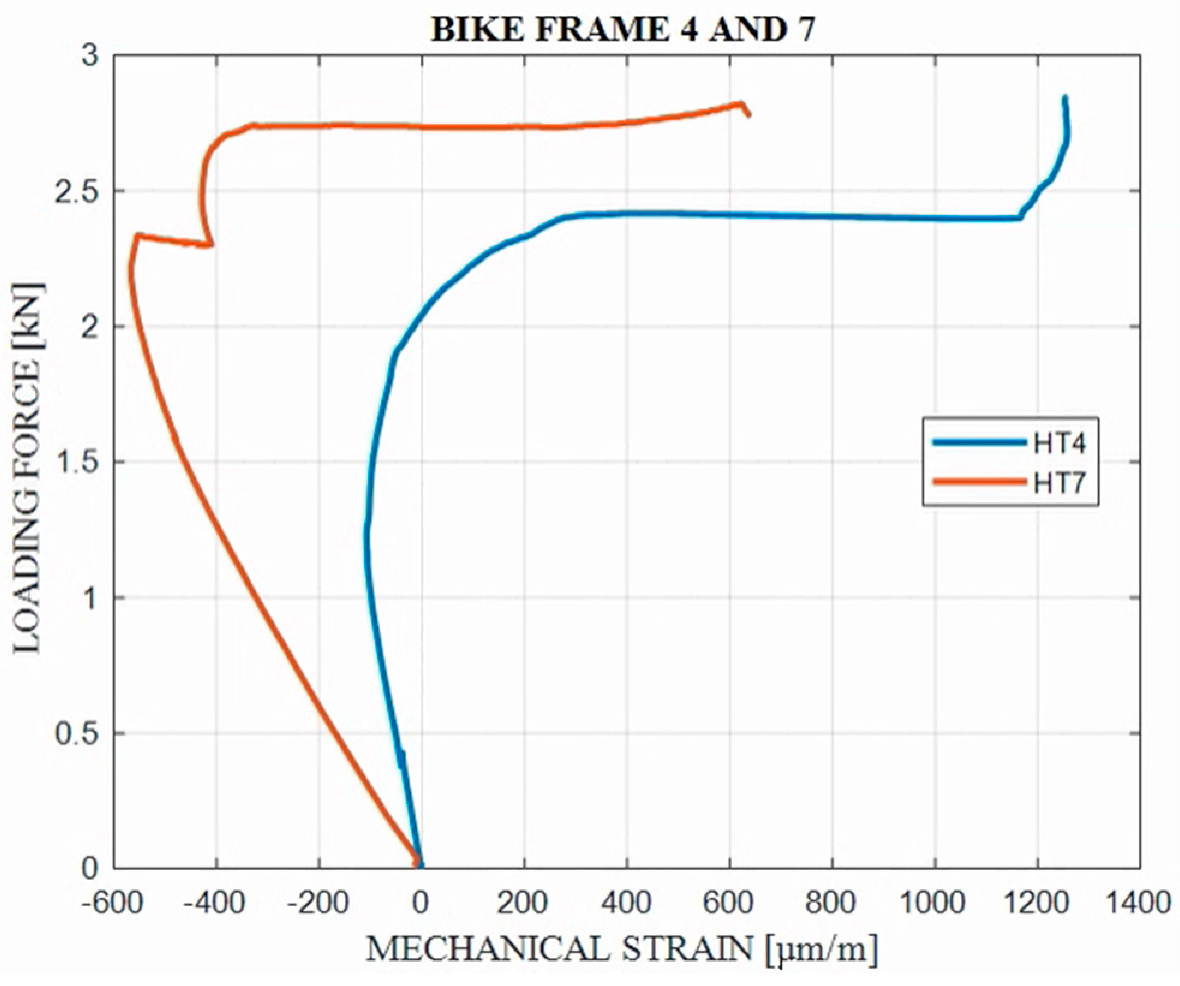
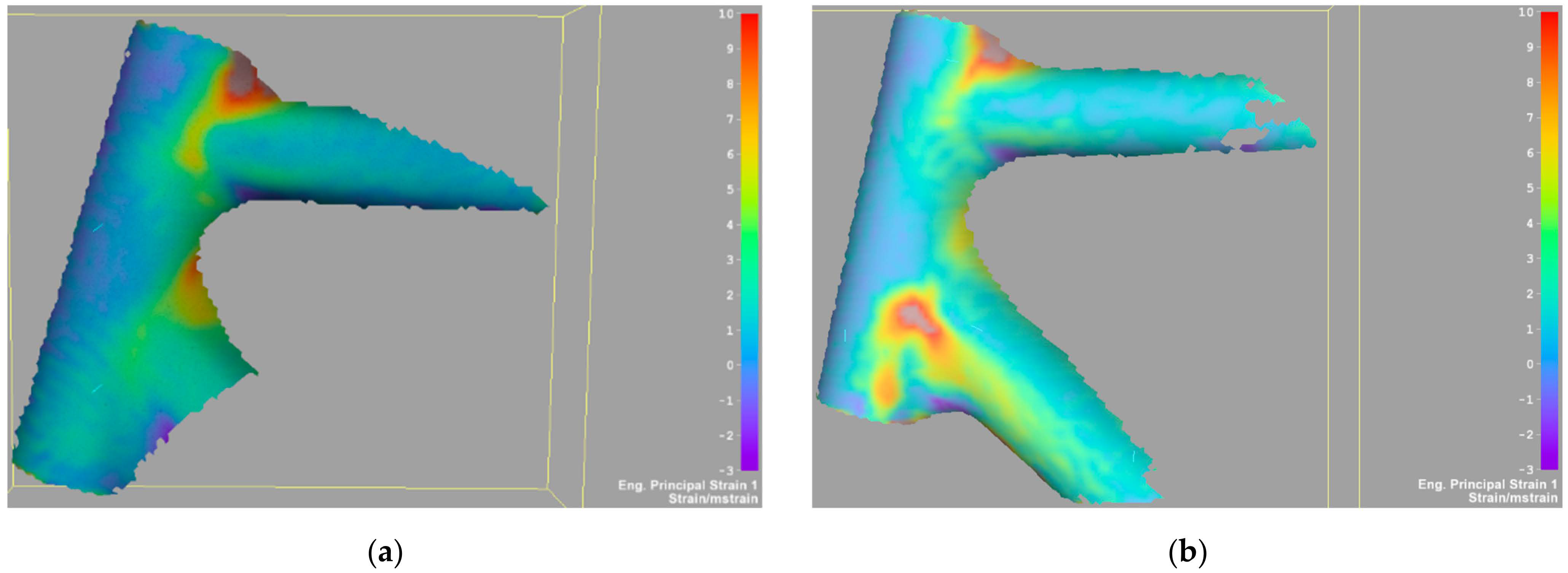
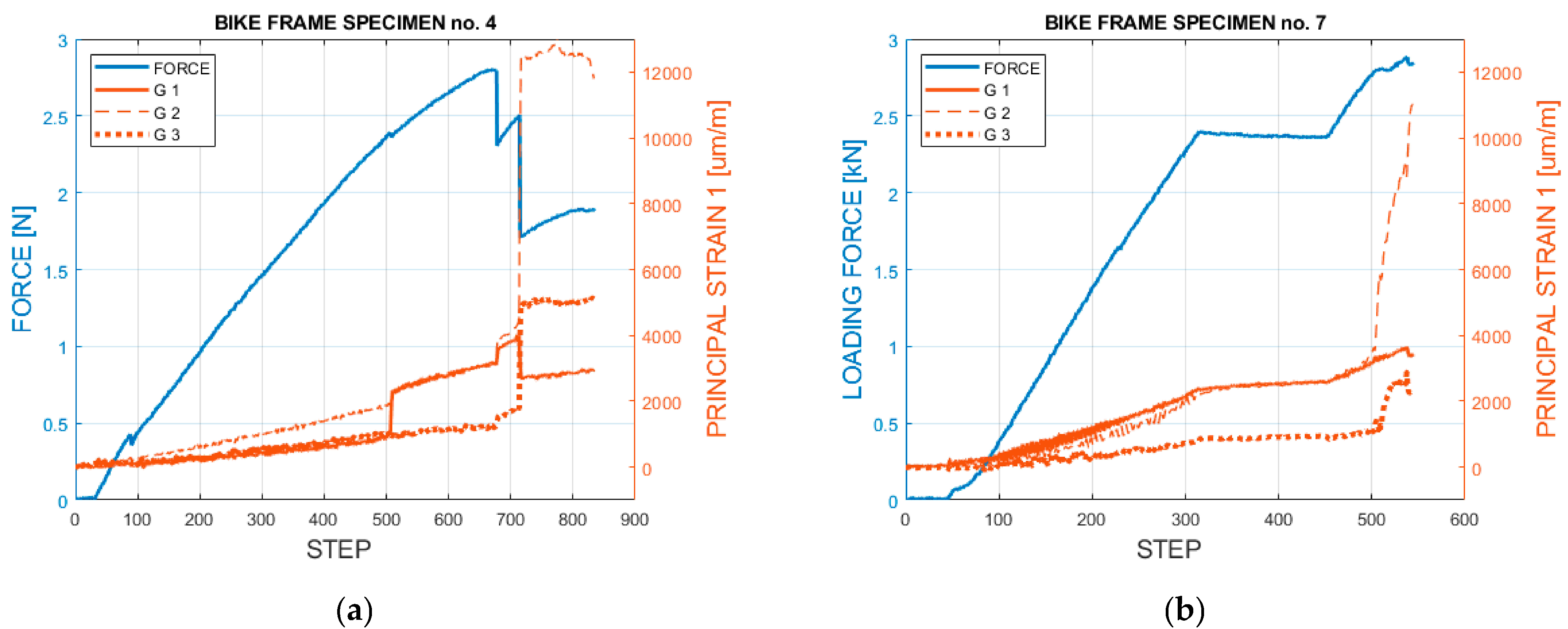
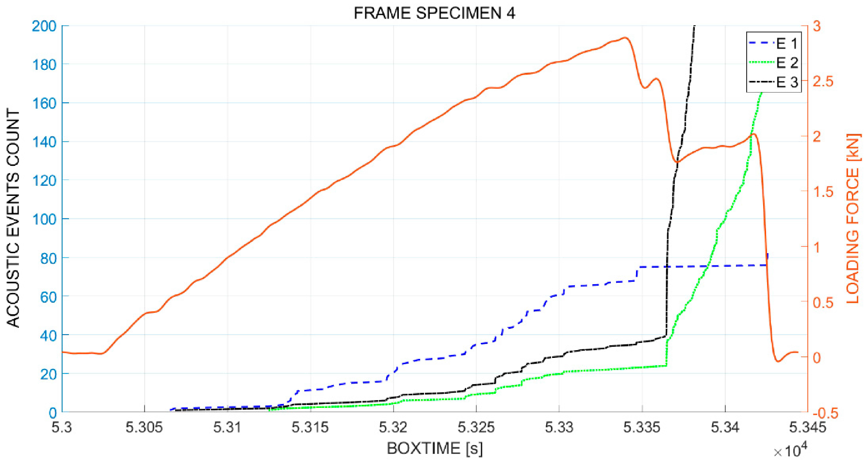
Horizontal forces—pushing load—specimens 1, 2, 4 and 7
Applsci 12 08377 i008
Simplified bicycle frame—specimens 1, 2, 4, 5, 6 and 7 The experimental work was focused on the most critical load case in terms of rider safety, in order to evaluate the behavior of the head tube joints area under a quasi-static testing to failure and to investigate the influence of its strengthening. Frame specimen 7 has a strengthened head tube joints area. This was achieved by using twice the number of fabric layers compared to frame specimens 0, 1, 2, 4, 5 and 6.
  • SG sensors
  • DIC
  • AE
Section 2.6.3Section 3.3
Horizontal forces—pulling load—specimens 5 and 6
Applsci 12 08377 i009
Table 2. Summary of experimental results for the FBG sensors.
Load Case ScenarioSpecimen No. @ Fmax [kN]Mechanical Strain [µm/m]Comments
FBG DTSG DTF34FBG TTSG TTF34
Pedal forcesframe specimen no. 0580388−480−364
Horizontal forces−210−7805Pushing load case
Vertical forces−151−114
Bottom bracket stiffness−371−376402375
Head tube torsion stiffness−267−117209117
Ergometer test963448−743−262
DIC, frame structural strength test1 @ −3.30−1576 33 Pushing load case, maximum strain values evaluated using DIC in FBG sensor areas
2 @ −2.90940 1100
4 @ −2.85−1800 1700
7 @ −2.87−2120 1095
Publisher’s Note: MDPI stays neutral with regard to jurisdictional claims in published maps and institutional affiliations.

