A Statistical Approach in the Analysis of Geometrical Product Specification during the Cold Tube Drawing Process

Abstract

Cold tube drawing provides higher accuracy compared to hot approaches. The process can be used to reduce the dimensions of tubes, and depending on the reduction size, the wall thickness of these may be subject to changes. In the process, any form of variability provoked by external factors is highly sensitive, given that the resulting tubes are often the final step in tube production. This paper focused on the evaluation of the influence of pre-tube factors on key variables after the drawing process, i.e., the final roundness, outer diameter, and wall thickness of the tubes. For these purposes, a factorial design with fixed factors was implemented. It was also a goal to investigate if the single-pass type of drawing would guarantee good statistical results potentially leading to significant time and financial reductions. The measurements were executed in the machine ZEISS CenterMax. The statistical analysis took place on Minitab 19. The results prove that most factors, and their interactions, significantly impacted the response variables, leading the authors to understand that a single-pass approach would not properly work under the conditions defined for the experimentation. These results also allow for reflection on the causes and necessary measures related to lubrication, technological heritage, and quality that would impact the results themselves.

1. Introduction

Over the years, the production of tubes has had a tremendous importance for industry. A clear example of this is the automotive sector, which is the fuel for many European economies such as the Slovak economy. Usually, tubes are either produced by cold or hot approaches, and depending on the production process or the intended final use of the tubes, there are either loose or increased demands for the accuracy of the tubes’ dimensions. In the case of precision steel tubes, these have a narrower tolerance field of diameters as well as wall thicknesses, and thus, in this specific case, there is an increased demand for precise production environments where the correct selection of process parameters and the very construction of the drawing tool play a major role. This cold forming process achieves a higher surface quality and higher dimensional accuracy of tube production compared to hot forming. The principle of cold tube drawing is analyzed in detail in [1,2,3,4].

Cold tube drawing, as a production process, focuses on the reduction in tube dimensions as well as the tube outer and inner diameters, while the process of plastic change of shape, i.e., reduction in tube cross-sections, is carried out by the drawing tool (also known as a die). The shape and dimensions of the die are the key factors in meeting the requirements for the geometric accuracy of the final tube and the roughness of its surface. In the state of the art and the practice, there are several scientific publications which have been aimed at optimizing the shape of the die and monitoring the influence of the die geometry on the final quality of precision tube production using finite element analysis [5,6,7,8].

Similarly, in this particular field, numerical simulation is also known for being an important tool for monitoring the plastic flow of the material in the drawing tool during cold tube drawing. Moreover, it also allows for optimizing process and technological parameters and predicting their possible effects on the accuracy of the tube production process, as stated in [9,10,11,12,13,14,15,16].

Another important parameter that influences the accuracy of drawn tube dimensions is the plastic strain degree (also known as reduction), i.e., a relative change in cross-sections. In cold tube drawing, it is also necessary to compare the actually achieved strain values with the limit values, because exceeding the limit degree of strain leads to the failure of the tube or the occurrence of defects on its surface. Additionally, the flawlessness of tube drawing is also affected by the plasticity and formability of the drawn material, as these affect the limit of plastic deformation and thus the number of drawing operations required to produce tubes of the required dimensions. The limit of formability in conventional tube drawing has been published in, for example [17]. This research clearly investigated the potential for optimizing the cold drawing process of steel tubes by reducing the number of drawing operations while minimizing residual tensile stresses, which is particularly important and closely related to some of the goals of this paper.

On the other hand, even though, at present, the application of statistical methods continues to prove its great potential for a fast and reliable evaluation of dimensional and shape deviations of drawn tubes, this potential is not yet sufficiently used in production processes and metrology activities, which is detrimental because of its great importance for the production sphere, especially in terms of reducing the failure of production, increasing the certainty of measurement experiments, and reducing production costs.

Moreover, the proper evaluation of the quality of production of drawn tubes requires the development of methodological approaches that incorporate and use such statistical methods to predict and/or at least better understand the technological impacts that pose the greatest risk of non-compliance with tube dimensions and shapes within permitted tolerances for precision production. This is something that is poorly addressed in the state of the art and the practice or that, at least, has not been published for the specific case of the cold tube drawing process under study in this paper. This finding alone remains a gap worth covering and solving in the scientific literature, and thus it is also one of the main motivations behind this paper.

In this paper, the authors investigated how the selected factors, with their respective levels of interest and their interactions, affect a certain number of output or response variables after the cold tube drawing process, i.e., the roundness of the tube, the final outer diameter of the tube, and the final or resulting wall thickness of the tube, which is a result of the difference between the final outer and inner diameters of the tubes. These are all key indicators commonly taken into consideration when assessing the overall accuracy and quality of cold tube drawing, which have been reported to be vital and worth studying by many key tube manufacturers in the country.

As for the statistics behind all this, based on the authors’ own experiences and an up-to-date analysis of the state of the art and the practice, it is possible to conclude that the arsenal of statistical tools, methods, and/or approaches that could be used for the analysis of cold tube drawing experiments such as the one discussed in this paper is quite vast. These methods range from very simple ones to those of a more complex nature, and thus the problem of properly selecting the one that better fits the needs of a problematic situation and that provides a given case study with the correct solution or verification strategy has also become a complex task.

One of the commonly used approaches is, for example, the use of the well-known linear or multiple regression models, as used in [18], or even [19]. These models are, in essence, defined by the fact that they allow estimating the relationships between a dependent variable and one or more independent variables. However, after a thorough examination of them and trying to make them fit into the intentions of this paper, the authors came to the conclusion that even when an approach such as this would offer valuable information, it would not help in carefully analyzing the specific levels of interest investigated under this study, and that several independent regression models would be needed for individually exploring combinations of independent variables to yield a better regression result for the studied dependent variables, which is not the aim of this research. Similarly, the inadequacy of solely focusing on regression analysis for the purposes of this research becomes even more evident if taking into account that the levels under study belong to finite and discrete realms or populations; thus, interpreting the results of regression models would be a difficult task to realize, and several compromises and abstractions inducing subjectivity would also be needed if obtaining values out of the discrete scale defining the levels of a factor, with the added impossibility of analyzing interactions and/or combinations among all of these levels.

On the other hand, there are also several optimization or multi-objective optimization approaches that could be used for the purposes of this paper: for example, under the assumption that the authors considered the problem a multi-response problem, some approaches can be found in [20] or in [21], as well as the way these authors covered this topic, and the many solution strategies or methods they found for it, e.g., the contour plot overlay strategy, the constrained optimization problem approach, and the use of desirability functions. However, even though using strategies such as these in the case of this paper could be useful to an extent, their complexity and the nature of what is intended to be investigated in this research would not yield the expected results; thus, these methods would not be the correct option given that, as mentioned before, the authors are not looking for the best value of an infinite continuous population of levels allowing for achieving the best response, but instead they are strictly investigating specific levels of interest, and thus finding any other level value other than the studied ones may be irrelevant to what is intended to be demonstrated and investigated with this research.

Even though the authors of this paper could continue to mention and review several other methods they found in the state of the art and the practice, and that could offer some value to this research and contribute to the goal of the paper, they generally believe that the well-known design of experiments (DOE) technique, and more specifically the factorial designs within it, is the method that best fits this research’s needs. These factorial design techniques are very often used in experiments consisting of several factors where it is necessary to analyze the joint effect of the factors on a given response, and this is precisely the case of this research.

As for the use of statistical methods concerning DOE and factorial designs in the specific area of the cold tube drawing process, also known as free tube sinking, or simply tube drawing, there has not been a significant number of publications in recent years. For example, in the case of [22], the authors focused on the tube sinking process using a conical die for the case of tubes made of polymeric materials. In their paper, they implemented a finite element study and designed an experiment where they studied the influence of factors such as the drawing speed, tube wall thickness, die/tube friction, die reduction, and die semi-cone angle on only a single response variable, namely, the drawing loads.

Similarly, the authors of [23] also presented a somewhat similar and common take on the analysis of the cold tube drawing process by first conducting some mathematical simulations and subsequently using the resulting data for the experimental analysis. These authors mainly focused on studying and searching for the best geometries of the die and plug in order to reduce the drawing force, and although they claimed to have presented a random factorial analysis, they did not offer much proof of it or properly explain the randomness of the factors’ levels, or the scientific, mathematical/statistical, and experimental base behind their conclusions and results of the experimental analysis.

On the other hand, the authors of [24] presented a three-dimensional finite element model which was developed to help them calculate the change in the wall thickness, eccentricity, ovality, and residual macro-stress state of the tubes, produced by the same cold drawing process, in the presence or absence of a plug. These authors also carried out an experiment in order to validate their simulation results; however, they did not carry it out in the way it is conceived within this paper given that they missed or did not need a proper design for the experiment itself.

As mentioned in [20], out of the many special cases of factorial designs, the most important factorial design is that having k factors, each at only two levels, i.e., the 2^k type of experiment. These levels may be quantitative, such as two values of temperature, pressure, or time, or they may be qualitative, such as two machines, two operators, the “open” and “close” levels of a factor, or perhaps the presence and absence of a factor. In the case of this paper, these factors refer to: (1) the wall thickness of the pre-tube, (2) the diameter of the pre-tubes (also known as draft tubes), and, finally, (3) the diameter of the die. As opposed to what was presented and published by some of the authors of this paper [25], factors, and their levels here, are to be considered fixed, meaning that there is no randomness in their selection, but instead, they are all specific levels of interest needing to be studied in the experiment.

It is important to mention that in the 2^k type of experiment, there is a need to assume that: (1) the factors are fixed, (2) the designs are completely randomized, and (3) the usual normality assumptions are met. All of these assumptions are to be tested for the case study in the context of this paper.

On the other hand, the 2^k design is particularly useful in the early stages of experimental work when many factors are likely to be investigated, given that it provides the smallest number of runs with which k factors can be studied in a complete factorial design, and this is precisely the reason why these 2^k designs are commonly used when screening factors in experiments such as the one presented in this paper, as the intention is mainly to discover the active factors and/or their interactions from a larger population of factor candidates.

Based on all previously discussed facts and elements, approaches, and theories constituting the problematic situation motivating this research, the authors of this paper noticed that a study such as the one presented in this document has not been carried out in the state of the art and the practice. This affirmation becomes even stronger if making it specific to the case of the cold tube drawing process itself. The authors also noticed that there is a lack of methodological tools that would guide practitioners and the interested community in properly implementing DOE techniques, with emphasis on the factorial designs, in the design, analysis, evaluation, and improvement of the cold tube drawing process involving coordinate measuring machines (CMMs), and in drawing key conclusions on key factors and their interactions and how these affect relevant post-cold tube drawing process parameters. These elements are, in essence, the goals to address in this paper and constitute, at the same time, the main scientific problem to solve.

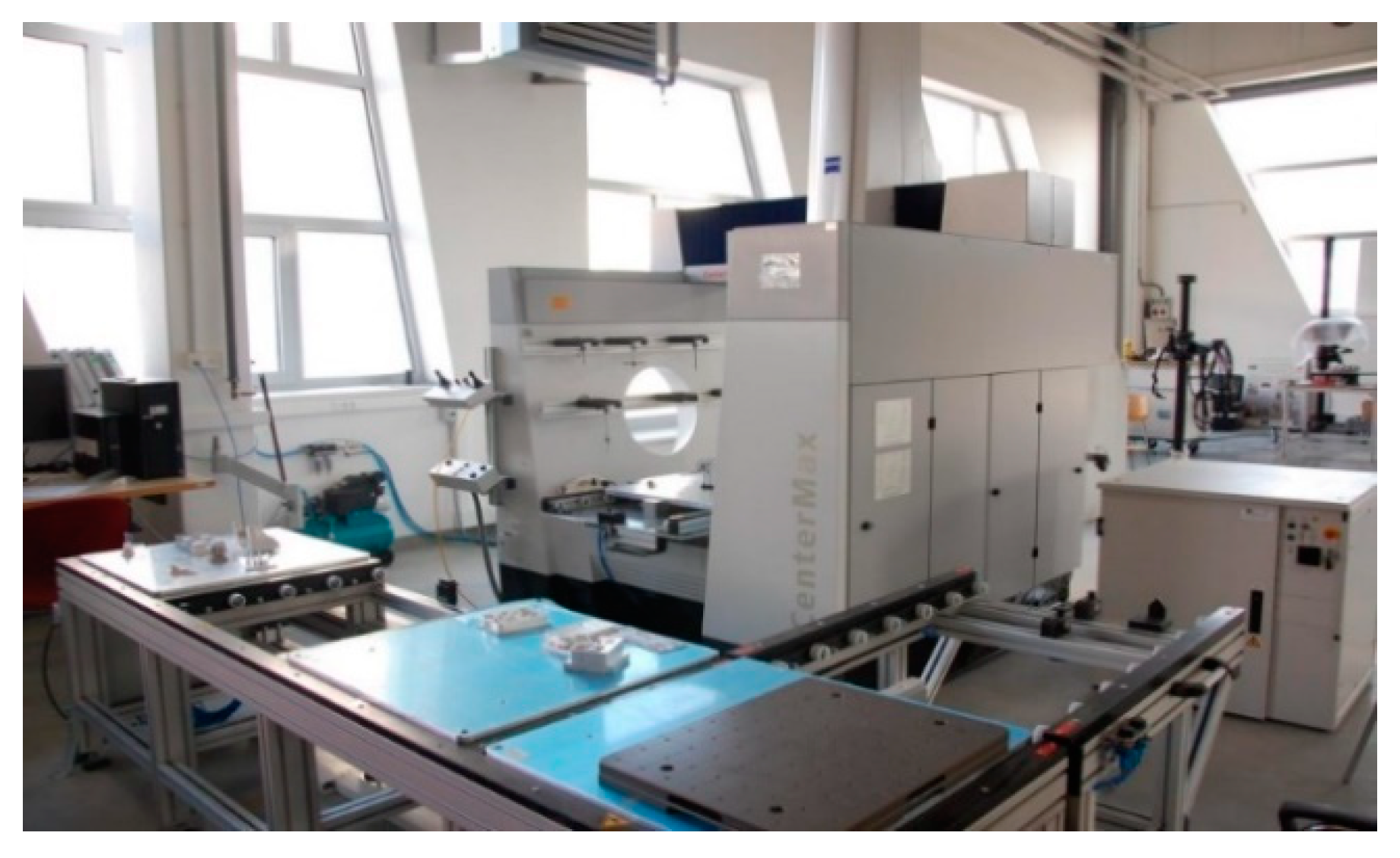
The measurements for the experiment of this paper were obtained using a ZEISS CenterMax CMM, which is located at one of the laboratories of the Faculty of Materials Science and Technology in Trnava, Slovakia. The remainder of this paper is divided into the following sections: Section 2, Materials and Methods; Section 3, Results and Discussion; Section 4, Conclusions; and finally, there is a References section containing all of the up-to-date literature consulted for the purposes of the research in this paper.

2. Materials and Methods

As briefly mentioned in the introduction of this paper, when analyzing the available materials in the state of the art and the practice, one can usually find many tools, methods, and/or approaches to design an experiment. Some of the most powerful and important methods are those known as factorial designs, which can be found, for example, in [26], where this well-known author recreated and detailed DOE techniques, with emphasis on such factorial designs, and explained that within these designs, experimental or response variables are investigated through all or part of all possible combinations of the related factors at their different levels, and the results are then subsequently analyzed by a technique known as analysis of variance (ANOVA).

In consequence, as stated in [25], this group of techniques has received a remarkable share of attention from the scientific community given their many applications and their contributions to a profound analysis, understanding, and even quantification of the impact of experiments’ factors and their interactions, at all or several levels, on a given response variable through the strategy of experimentation.

In the literature consulted for this paper, there are, of course, several more authors who have covered, in detail, some theories and applications in terms of DOE using factorial designs: for example, [27,28,29], and most of Montgomery’s saga editions, especially [20,26,30], were consulted for this paper.

Moreover, one way or another, most of these publications also addressed the importance of properly designing the experiments, and in consequence, they even defined clear steps that are to be considered in this process. Given that the authors of this paper mostly agree with the steps and/or guidelines presented in these sources and understand the relevance of a properly conceived design, they likewise followed similar guidelines for the purposes of the experiment in this research and decided to present their own version, as shown below in

Table 1. General guidelines for designing an experiment.

Guidelines	Some Explanatory Notes
1. Identification and definition of the problem	This is often the most important part in the success of a given experiment, often being associated with Pareto’s principle. It is key to define what the experiment is useful for, e.g., factor screening, optimization, validation, or reaffirmation of something suspected.
2. Identification and definition of the response variable	Selecting a contradictory response variable will always lead to inappropriate results. The experiment must also decide how to measure its value.
3. Identification and selection of factors and their levels	The number of factors and their levels have a connection with the logics and precision of the experiment. They are usually fixed or random, or mixed in some cases.
4. Selection of the type of experimental design	Curvature must be kept in mind when selecting an experimental design. The same selection is closely related to step 1. The experimenter also needs to define how many replicates are needed or can be executed, as well as the order of combinations or treatments and the order of the model.
5. Execution of the experiment	This implies selecting and properly setting up the experiment equipment, making sure the levels are properly set and even executing trial tests before the real experimentation begins.
6. Selection of the measurement device or system and definition of a proper measurement plan	This often depends on the final or technical resources available. The lower the mean percentage error of the equipment, the better. The equipment should be able to execute the measurements of all defined variables.
7. Selection of proper statistical software for the analysis of the collected data	This often depends on the final or technical resources available. The experimenter is advised to use professional software such as Minitab, IBM SPSS, and Statgraphics.
8. Interpretation of the results from the statistical analysis	This is one of the most important parts. Interpretations should be established strictly following the statistical theory; however, this should be carried out in the context of the given instance under study.

. Since this is not a book but a research paper, the authors kindly advise potential readers to refer to any of the previously mentioned authors for a description of these or similar guidelines, with special emphasis on [20], who covered this in detail.

Even though all of the previous steps in the guidelines are important and constitute a whole, it is precisely the selection of the experimental design which is considered to be a milestone in any experimental design, given that it may make the experiment either stand out or worthless. For these purposes, it is also of particular importance to consider the time available for the realization of all experimental runs. This time has a direct relation to the number of experimental variables, the number of their levels, and the amount of data required.

In a factorial design, the runs are usually represented by the value of n, which refers to the number of combinations and can be easily determined using the expression n = l^k, where l stands for the number of levels of the factors, and k refers to the number of experimental variables investigated (factors). For example, if conducting an experiment with three factors at two levels each, such as the one presented by the authors of this paper, the total number of runs or combinations would be 2³, which yields a total of 8. At the same time, this value of n must always be multiplied by the number of replicates of the experiment. These replicates are known to be extra experimental runs with the same factor settings (levels), subject to the same sources of variability and/or conditions independently of each other.

The authors of, for example, [20,31], and even Minitab 18´s support website [32], which is the software used for the statistical analysis in this paper, generally agree on the fact that the sample size of an experiment depends on (1) the size of the effects, (2) the choice of type I error, and (3) the power of the statistical test to be achieved. Even though the first and second criteria may always depend on the specificities of a given experiment, in the case of the third criterion, all of these works further state that the sample size should usually be able to yield a power (level of confidence) of more than 0.8 or 80%, while at the same time, these authors, and those of this paper, also agree on the fact that the bigger the number of replicates and size of the experiment, the better the chance the experimenter has to recognize smaller effects or simply increase the level of confidence of the whole design.

In this sense, based on the authors’ experience and several published works with similar experiments, for example, [20,26], where one can find some examples, an experiment of the 2³ type is usually sufficient, with simply two or three replicates. However, in the case of this paper, the number of replicates was defined as four for two of the variables and three for the last one, and this was due to the fact that the authors wanted to guarantee a better analysis of the factors, and they mostly took into account the necessary monetary resources and time for the realization of all the measurements.

As it has been mentioned before, the fact that the authors of this research opted to implement a factorial design-based DOE as the best course of action reflects their interest in and need for studying the joint effect of three specific factors and their interactions on given response variables. Analyzing more than a single response variable often leads to solution alternatives, which, in this case, translates to the decision of the authors to elaborate three separate 2^k designs which are described and analyzed in detail later in this document.

On the other hand, despite the existence of several variations or types of factorial designs, the authors specifically decided to implement one of the 2³ type, and this was mainly for two reasons: (1) it fits the needs of the study, and (2) this type of design has been shown to be superior to other alternatives such as the 3^k type, as discussed, for example, in [20].

The author of [20] also presented a very detailed and generally well-accepted sequence of steps for the realization of this type of design, and thus the experiment that was carried out in this paper was in accordance with his proposed “Analysis Procedure for a 2^k design”, which was slightly modified by the authors, as follows:

• Estimate the effects of the factors and their interactions;
• Form the initial model:
  • If the design is replicated, fit the full model;
  • If there is no replication, form the model using a normal probability plot of the effects;
• Perform statistical testing using the selected software (generally ANOVA testing);
• Refine the model (non-significant variables may be excluded from the model);
• Analyze residuals and verify the model adequacy and fulfilment of the assumptions;
• Interpret the results using proper plots (main effect and interaction plots, response surface and contour plots).

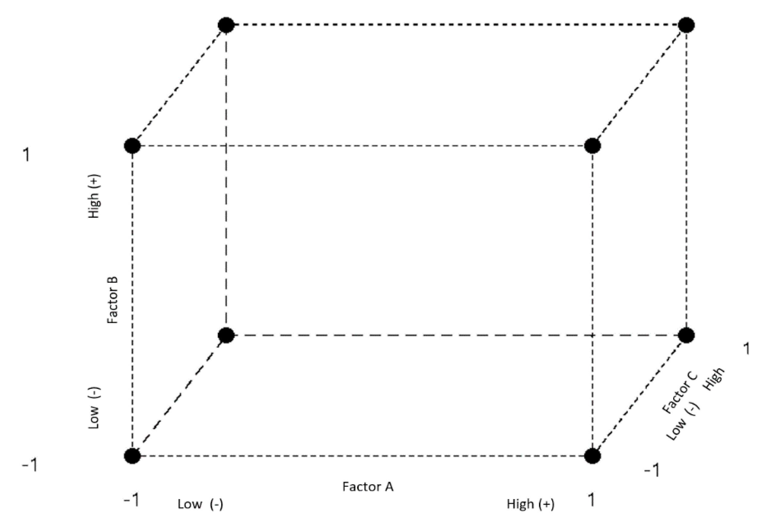
The statistical model for a 2^k design includes k main effects, $\left(\begin{array}{c}k\\ 2\end{array}\right)$ two-factor interactions, $\left(\begin{array}{c}k\\ 3\end{array}\right)$ three-factor interactions, and one k factor interaction. In the case of our 2³ design, if applying the commonly used letter or label notation, it can be interpreted as follows: a, b, and c are the main effects; ab, ac, and bc are the two-factor interactions; abc represents the three-factor interactions; and, finally, (1) is the k factor interaction. The following

Table 2. Experiment table of 2³ design with the most commonly used notations.

Run	A	B	C	Labelling	A	B	C
1	-	-	-	(1)	0	0	0
2	+	-	-	a	1	0	0
3	-	+	-	b	0	1	0
4	+	+	-	ab	1	1	0
5	-	-	+	c	0	0	1
6	+	-	+	ac	1	0	1
7	-	+	+	bc	0	1	1
8	+	+	+	abc	1	1	1

shows the general experiment table for a 2³ design. This table is also known as the design matrix of the experiment if using the + and − notation (orthogonal coding). In the table, it is also possible to see two other common notations which are also used in terms of DOE.

Similarly, the following Figure 1 shows the geometric view of a general 2³ design.

On the other hand, if the experiment is replicated n times, the observations could also be described by a linear model, as shown in Equation (1).

$$\begin{array}{cc}\begin{array}{c}{y}_{ijkl}=\mu +{\tau }_i+{\beta }_j+{\gamma }_k+{\left(\tau \beta \right)}_{ij}+\\ {\left(\tau \gamma \right)}_{ik}+{\left(\beta \gamma \right)}_{jk}+{\left(\tau \beta \gamma \right)}_{ijk}+{\epsilon }_{ijkl}\end{array}& \{\begin{array}{c}i=1,\dots a\\ j=1,\dots b\\ \begin{array}{c}k=1,\dots c\\ l=1,\dots n\end{array}\end{array}\end{array}$$

(1)

where $y_{ijkl}$ represents the observed variable, for example, the resulting roundness or the final outer diameter of a tube; ${\tau }_i$ is the effect of the i-th level of factor A; ${\beta }_j$ is the effect of the j-th level of factor B; ${\gamma }_k$ is the k-th level effect of factor C; and ${\left(\tau \beta \right)}_{ij}$, ${\left(\tau \gamma \right)}_{ik},{\left(\beta \gamma \right)}_{jk},{\left(\tau \beta \gamma \right)}_{ijk}$ represent the effects of the interaction between factors. Similarly, the letters a, b, and c refer to the number of levels for each factor, r denotes the number of replicates, and ${\epsilon }_{ijkl}$ is a random error component. Despite the fact that all of the parameters of the model are independent of the error ${\epsilon }_{ijkl}$, they are all normally distributed, with a mean and value of variance of zero, expressed by NID (0,${\sigma }_T^2$). In consequence, the variance of any observation is given by Equation (2).

$${\sigma }_y^2 ={\sigma }_{\tau }^2 +{\sigma }_{\beta }^2+{\sigma }_{\gamma }^2+{\sigma }_{\tau \beta }^2+{\sigma }_{\tau \gamma }^2+{\sigma }_{\beta \gamma }^2+{\sigma }_{\tau \beta \gamma }^2+{\sigma }^2$$

(2)

Moreover, if assuming all factors of a given experiment are fixed, as is the case of the case study in this paper, then the ANOVA can be defined as presented in the following

Table 3. Analysis of variance for the general case of the three-factor model with fixed effects.

Source of Variation	Sum of Squares	Degrees of Freedom	Mean Squares	Calculated F
A	SSA	a − 1	$MSA=\frac{SSA}{DFA}$	$F=\frac{MSA}{MSR}$
B	SSB	b − 1	$MSB=\frac{SSB}{DFB}$	$F=\frac{MSB}{MSR}$
C	SSC	c − 1	$MSC=\frac{SSC}{DFC}$	$F=\frac{MSC}{MSR}$
AB	SSAB	(a − 1)(b − 1)	$MSAB=\frac{SSAB}{DFAB}$	$F=\frac{MSAB}{MSR}$
AC	SSAC	(a − 1)(c − 1)	$MSAC=\frac{SSAC}{DFAC}$	$F=\frac{MSAC}{MSR}$
BC	SSBC	(b − 1)(c − 1)	$MSBC=\frac{SSBC}{DFBC}$	$F=\frac{MSBC}{MSR}$
ABC	SSABC	(a − 1)(b − 1)(c − 1)	$MSABC=\frac{SSABC}{DFABC}$	$F=\frac{MSABC}{MSR}$
Residual	SSR	abc(n − 1)	$MSR=\frac{SSR}{DFR}$
Total	SST	abcn−1

. This table has been taken and modified from [25], who cited it, modified it, and took it from [20] at the same time. For a more detailed take on the calculation of the sum of squares, the readers of this document are kindly advised to refer to the content starting from page 201 in the work of the last of the mentioned authors.

Since a key part of a factorial design of this type relies on the initial calculation of the effects and their interactions, and since these are sometimes to be manually calculated in order to possibly corroborate ambiguous computer results, the authors present a set of equations for the calculation of such effects. As it can be seen, the parts of the equations in square brackets refer to the contrasts. The calculation of the effects is also key for the calculation of the sums of squares.

$$A=\frac{1}{4n} \left[a+ab+ac+abc-\left(1\right)-b-c-bc\right],$$

(3)

$$B=\frac{1}{4n} \left[b+ab+bc+abc-\left(1\right)-a-c-ac\right],$$

(4)

$$C=\frac{1}{4n} \left[c+ac+bc+abc-\left(1\right)-a-b-ab\right],$$

(5)

$$AB=\frac{abc+ab+c+\left(1\right)}{4n}-\frac{bc+b+ac+a}{4n},$$

(6)

$$AC=\frac{1}{4n} \left[\left(1\right)-a+b-ab-c+ac-bc+abc \right],$$

(7)

$$BC=\frac{1}{4n} \left[\left(1\right)+a-b-ab-c-ac+bc+abc \right],$$

(8)

$$ABC=\frac{1}{4n} \left[abc-bc-ac+c-ab+b+a-\left(1\right)\right],$$

(9)

On the other hand, in a 2³ design, each effect has a corresponding contrast with a single degree of freedom, while if there are n replicates, the sum of squares for any effect may be determined as follows:

$$SS=\frac{specific contrast}{8n},$$

(10)

Although, in a factorial design of this type, the impact of the factors and their interactions (the model terms) on the total sum of squares is usually more precisely verified using the ANOVA tool, it is sometimes also important to obtain a rough value of it, as defined by the following Equation (11):

$$Percent contribution of the term relative to the total SS=\frac{SS of the term}{Total SS},$$

(11)

Another important formulation in terms of a design of this type is the regression equation. This usually only includes the model terms that have been proved to be significant in terms of their p-values in the ANOVA results. The following Equation (12) shows an example of a regression equation for the specific case of a 2³ design, such as the one described further in this paper; however, using a similar analogy may allow the experimenter to modify this equation and make it fit any other design type.

$$y={\beta }_0+{\beta }_1{x}_1+{\beta }_2{x}_2+{\beta }_3{x}_3+{\beta }_{12}{x}_1{x}_2+{\beta }_{13}{x}_1{x}_3+{\beta }_{23}{x}_2{x}_3+{\beta }_{123}{x}_1{x}_2{x}_{3 }+\epsilon$$

(12)

Last but not least, in this experimental design, there is a need to formulate the hypotheses for the experiment (see

Table 4. Formulation of the hypotheses.

Null Hypotheses	Alternate Hypotheses
H0$: {\sigma }_{\tau }^2=0$	${\mathrm{H}}_1 {\sigma }_{\tau }^2>0$
H0$: {\sigma }_{\beta }^2=0$	${\mathrm{H}}_1 {\sigma }_{\beta }^2>0$
H0$: {\sigma }_{\gamma }^2=0$	${\mathrm{H}}_1 {\sigma }_{\gamma }^2>0$
H0$:{\sigma }_{\tau \beta }^2=0$	${\mathrm{H}}_1 {\sigma }_{\tau \beta }^2>0$
H0$:{\sigma }_{\tau \gamma }^2=0$	${\mathrm{H}}_1 {\sigma }_{\tau \gamma }^2>0$
H0$:{\sigma }_{\beta \gamma }^2=0$	${\mathrm{H}}_1 {\sigma }_{\beta \gamma }^2>0$
H0$:{\sigma }_{\tau \beta \gamma }^2=0$	${\mathrm{H}}_1 {\sigma }_{\tau \beta \gamma }^2>0$

). In the case of a 2³ design type such as the one addressed in this paper, the hypotheses to be defined are shown below. These hypotheses can be evaluated or tested using any of the different means for such purposes, e.g., the F₀ statistic from the ANOVA results, as presented in Table 3, or the p-values (see [20]).

2.1. Particularities of the Factorial Designs under Study

As briefly mentioned before, the factorial experiment presented in this section and its subheadings focused on the analysis of the cold tube drawing process in order to study the potential impact and/or influence of three factors over certain response variables. The design consisted of three fixed factors at two levels each, yielding a total of eight treatments. The factors were defined as (A) the diameter of the pre-tube (also known as the draft tube), (B) the wall thickness of the pre-tube, and, finally, (C) the diameter of the die. Given that the authors mostly took into account the necessary financial resources and time, a total of 4 replications were executed for variables y₁ and y₃, and 3 for the variable y₂, which resulted in a total of 32 and 24 runs, leading to a more robust take on the process under study and, of course, meeting the requirement of a minimum of 20 data entries suggested in Minitab for analyzing the normality assumption of the data. On the other hand, since the authors wanted to study the effect of these factors on three concrete separate response variables, it was decided to define three separate 2³ factorial designs or cases for these purposes, as shown in

Table 5. General experiment design table for the case of the response variable y₁ (the roundness of the tube).

	Coded Factors			y1 (Final Roundness of the Tube in mm)
Run	A	B	C	Replicate 1	Replicate 2	Replicate 3	Replicate 4	Total
1	−1	−1	−1	0.0226715	0.0310896	0.0295886	0.0269921	1 = 0.087670
2	−1	−1	1	0.0519339	0.0539362	0.0516811	0.0538788	c = 0.159496
3	−1	1	−1	0.0465677	0.0478089	0.04385197	0.0457862	b = 0.137447
4	−1	1	1	0.03269045	0.0355279	0.0325575	0.0321517	bc = 0.100237
5	1	−1	−1	0.0782915	0.0748141	0.0701904	0.070804	a = 0.215809
6	1	−1	1	0.0942585	0.0956257	0.0965571	0.0921726	ac = 0.284355
7	1	1	−1	0.0147617	0.0150973	0.0164774	0.0167065	ab = 0.048281
8	1	1	1	0.0568767	0.0577252	0.05673148	0.05634873	abc = 0.170805

,

Table 6. General experiment design table for the case of the response variable y₂ (final outer diameter of the tube).

	Coded Factors			y2 (Final Outer Diameter of the Tube in mm)
Run	A	B	C	Replicate 1	Replicate 2	Replicate 3	Total
1	−1	−1	−1	11.9984635	12.0001687	12.0006063	1 = 35.999239
2	−1	−1	1	14.016702	14.016163	14.0168631	c = 42.049728
3	−1	1	−1	11.9826911	11.9828985	11.9822377	b = 35.947827
4	−1	1	1	13.97602	13.9774391	13.9772614	bc = 41.930721
5	1	−1	−1	12.0059696	12.0077322	12.0082373	a = 36.021939
6	1	−1	1	14.0143313	14.0135264	14.0139065	ac = 42.041764
7	1	1	−1	11.9878521	11.9881597	11.9884219	ab = 35.964434
8	1	1	1	13.9638494	13.965293	13.9667278	abc = 41.895870

,

Table 7. General experiment design table for the case of the response variable y₃ (the final wall thickness).

	Coded Factors			y3 (Final Wall Thickness of the Tube in mm)
Run	A	B	C	Replicate 1	Replicate 2	Replicate 3	Replicate 4	Total
1	−1	−1	−1	1.05110785	1.0518221	1.05324605	1.05204075	1 = 4.208217
2	−1	−1	1	1.0655571	1.065269	1.0655583	1.06576155	c = 4.262146
3	−1	1	−1	2.06992765	2.06936225	2.06844185	2.06980835	b = 8.277540
4	−1	1	1	2.1095563	2.11029615	2.1103695	2.11026285	bc = 8.440485
5	1	−1	−1	1.03527845	1.03550983	1.03543675	1.0359892	a = 4.142214
6	1	−1	1	1.0451128	1.04579615	1.04501635	1.04584755	ac = 4.181773
7	1	1	−1	2.10460995	2.1047688	2.1047449	2.1048271	ab = 8.418951
8	1	1	1	2.10704695	2.10657405	2.1068119	2.106388	abc = 8.426821

and

Table 8. General experiment design table for the case of the response variable y₁ (the final outer diameter of the tube)—factors’ levels.

Factors’ Levels
Factor, Measurement Unit	Low Value (−1)	High Value (1)
A (diameter of the pre-tube, mm)	16	18
B (wall thickness of the pre-tube, mm)	1	2
C (diameter of the die, mm)	12	14

. Notice, however, that Table 8 is common to all three designs, and thus it is only presented once. The response variables under study were denominated as y_r, where $r=\overline{1,o}$, and such variables were defined as the (1) the roundness of the tube, (2) the final outer diameter of the tube, and (3) the final or resulting wall thickness.

Case 1: Analysis of the factors and their interactions over the response variable y₁ (roundness of the tube).

Case 2: Analysis of the factors and their interactions over the response variable y₂ (the final outer diameter of the tube).

Case 3: Analysis of the factors and their interactions over the response variable y₃ (the final wall thickness).

Similarly, the following Table 8 shows the factors’ level table taken into account for the design. This table is common to all of the cases or factorial designs introduced above. These specific factors and their levels were selected for the study based on, among other issues, the fact that these were identified to be the ones more commonly present in key manufacturing and automotive-oriented processes in the area, which is vital for the Slovak economy given its strong orientation and dependence on this sector. These statements are backed up by the long-term experience and cooperation of most of the authors with relevant players in the tube manufacturing industry in the country, for example: Železiarne Podbrezová a.s., but especially by the fact that such companies have explicitly manifested their interest in these specific dimensions (factors and levels) given, again, their many uses and presence in industrial practice, and thus the need for a deeper study and understanding of their correlation and influence over certain specific indicators or response variables such as those analyzed within this paper (see, for example, [3], which partially addressed this need and importance previously).

On the other hand, it is also important to mention that the selected sizes of the tubes (outer diameters) and the dimensions of the die itself were also co-conditioned by the fact the above-mentioned company wanted to investigate, on a scientifically sound basis, the feasibility of a single-pass drawing approach given that it could not find relevant studies of this type on the issue, and that the authors of this paper could not find relevant approaches in the state of the art and the practice. In this regard, in order to obtain widely used tubes with final outer diameters of Ø12 and Ø14 mm, the authors selected pre-tubes whose outer diameters were not larger than Ø20 mm, given that this would not allow a safe and smooth single-pass drawing and would probably cause the tubes to break during the process, and this also constituted part of the reasons why pre-tubes with diameters of Ø16 and Ø18 mm and dies with diameters of Ø12 and Ø14 mm were selected for the study.

2.2. Description of the Experiment, Its Design Variables, and the Equipment Used

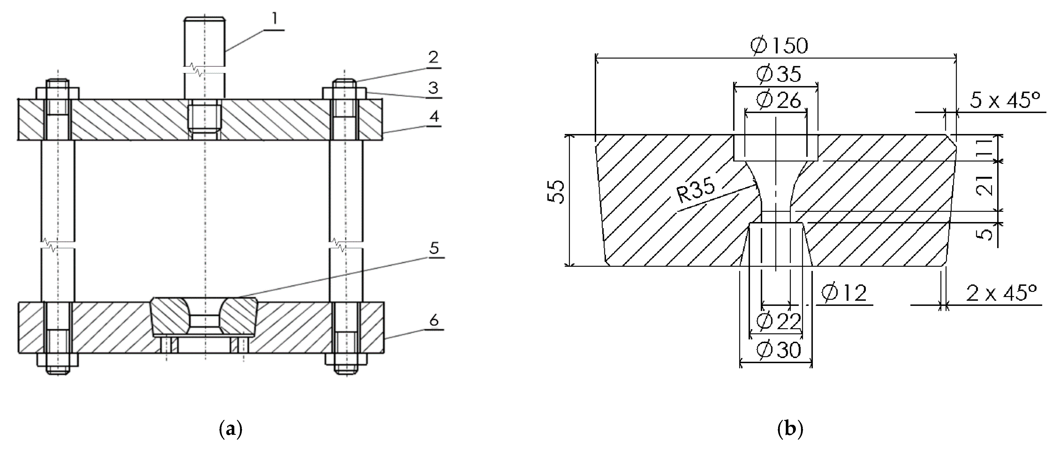
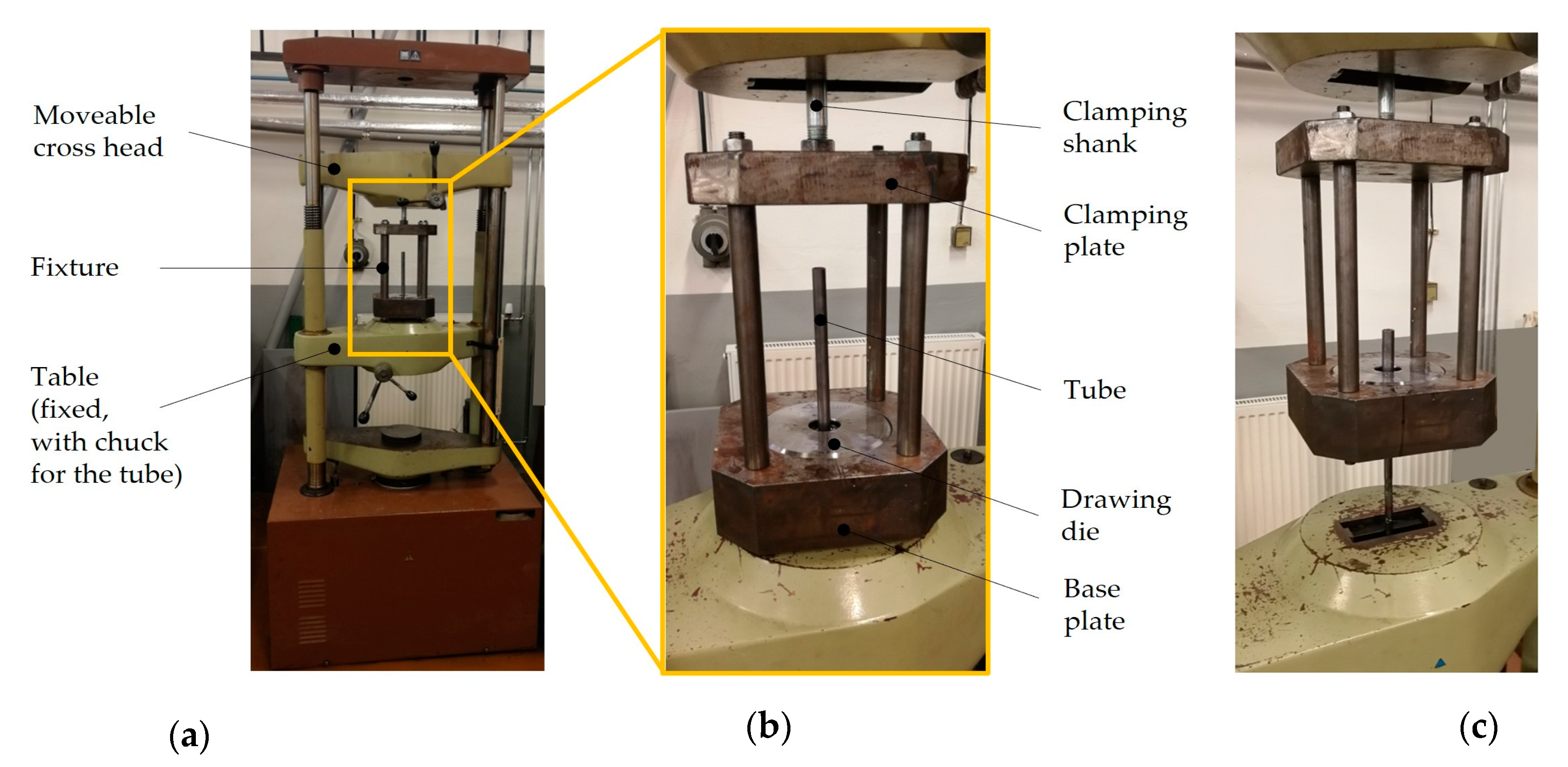
For the purposes of the laboratory experiment, a special fixture was designed and manufactured to perform the technological test of the drawing of seamless tubes (see Figure 2). Subsequently, the cold tube drawing experiment was performed in laboratory conditions using the EU 40 hydraulic testing machine with a nominal force of 400 kN (see Figure 3a).

As it can be interpreted from Figure 2, the drawing fixture consisted of individual components such as a clamping shank and a clamping plate, and also other technological parts such as a base plate in which the drawing die is centrally mounted. A detailed representation of the shape and dimensions of the drawing die used in the experiment is shown in Figure 2b. On the other hand, the fixture was structurally designed for clamping onto the workspace of the tensile testing machine. The method of clamping the fixture to the EU 40 testing machine is also documented in Figure 3. Here, it is possible to appreciate that the tube is firmly clamped in the chuck of the table of the hydraulic testing machine (by the swaged part of the tube) (see Figure 4), and the moveable cross-head displaces upwards with the fixture, i.e., with the drawing die (see Figure 3b,c). This way, in the experimental drawing, the drawing die moves instead of the tube.

Moreover, as part of the cold tube drawing experiment of seamless tubes, all test tubes were rotary swaged, numbered, and then used for direct drawing production (single-operation production). The drawing speed in each case was 60 mm/min, and a liquid lubricant mineral oil was applied to reduce the effect of friction.

As it can already be inferred from Table 5, Table 6, Table 7 and Table 8, during the experiment, a total of 8 test specimens were produced by the cold drawing process. Specimens 1 and 3 were drawn through the die to a final outer diameter of Ø12 mm, using draft tubes with values of the outer diameter of Ø16 mm for both and having wall thicknesses of 1 and 2 mm, respectively. Specimens 5 and 7 were also drawn through the die to a final diameter of Ø12 mm, while the dimension of the draft tubes’ outer diameter was Ø18 mm for both, and the wall thicknesses had values of 1 and 2 mm, respectively.

In the case of specimens 2 and 4, these were drawn using a die of Ø14 mm, both being pre-tubes of Ø16 mm and having wall thicknesses of 2 and 1 mm, respectively. The final two specimens, 6 and 8, were also drawn using a die of Ø14 mm, both being pre-tubes of Ø18 mm and having wall thicknesses of 1 and 2 mm, respectively.

As mentioned before, all of these elements constituted the factors engaged in the factorial experiments and their respective levels.

All of the response variables of the experiments were analyzed and/or measured using a CMM from ZEISS (ZEISS, Oberkochen, Germany) which is introduced further on in this paper. Even though explaining the essence of these variables may be quite simple and even unnecessary for some of the readers, especially the final diameter of the tubes, it is important to at least mention that the wall thickness was assumed to be the difference between the resulting or final outer diameter of the tubes after the drawing process. As for the roundness variable itself, the authors of [33], citing the ISO12181-1 standard, defined roundness tolerance as the zone between two concentric circles which enclose the circular profile. Moreover, they also defined a limit for the roundness deviations, which is the distance between two concentric circles touching and enclosing the extracted circle (i.e., measured points) at the minimum radial distance from each other (see also [25], which also covered and studied this variable).

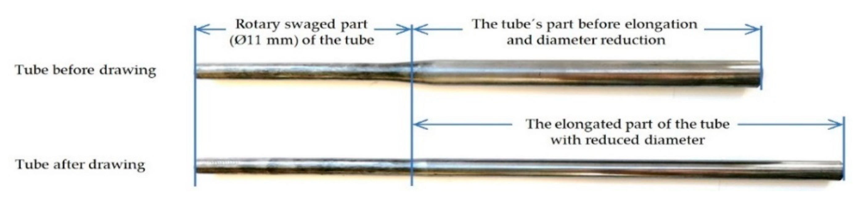
The shape of the tube before and after the drawing process is shown in Figure 4. The swaged part of the tube was used to clamp the tube to the chuck of the hydraulic tensile testing machine, EU 40, for the experimental drawing. The material used for the production of the drawn tube was low-carbon ferrite–pearlite steel (E235), which is suitable for the production of seamless tubes by cold drawing technology and is used in the automotive industry for the production of machine parts, or in the production of tubes for pressure, hydraulic, and pneumatic circuits. This E235 low-carbon steel has guaranteed weldability, good machinability, and also hot and cold formability. The material used in the experiment was delivered after a heat treatment process (normalizing), which took place between 890 and 950 °C. The chemical composition of the low-carbon E235 steel according to the EN10305-1 standard is presented in

Table 9. Chemical composition of E235 steel (wt %).

Element	C	Si	Mn	P	S	Cr	Cu	Mo	Ni	Sn
Composition	0.180	0.230	1.180	0.015	0.014	0.050	0.200	0.020	0.080	0.016

.

All of the measurements and data acquisition from the specimens obtained after the cold tube drawing process were carried out by the same experimenter, thus minimizing possible inconveniences, errors, and variability often attributed to multiple operators. In total, 32 and 24 runs were executed given that the 8 treatments underwent 4 (y₁, y₃) and 3 (y₂) replications, leading to more reliable results and a more robust experimentation, while also meeting the requirement of a minimum of 20 data entries suggested in Minitab for analyzing the normality assumption of the data.

The CMM in Figure 5 (ZEISS, Oberkochen, Germany) was used for obtaining all the data presented before in Table 5, Table 6 and Table 7; these data were used for the factorial designs. As also mentioned by some of the authors of this paper before in [26], this machine possesses a tactile sensor of the type VAST XTR gold and has a mean percentage error (MPE) between 1.2 + L/280 and 2.2 + L/180 µm for temperatures ranging between 20 and 40 °C, meaning that the CMM can operate in environment conditions ranging from 8 to 40 °C, offering better stability in measurements between +15 and +40 °C. The measurements within this study were all executed at room temperatures between 25 and 27 °C. This value of temperature also slightly depends on the season, and thus in other experiments, this value may vary up or down, although it always remains within the permissible optimal limits.

It is important to mention that the sequence of steps that defines the realization of the factorial experiments and the measurements obeys, to a great extent, the steps presented in Table 1 and those appearing before Figure 1.

3. Results and Discussion

The formulation of the hypotheses for the specific cases of all terms in the 2³ factorial designs presented in this paper are explicitly formulated in Table 4; however, now, the terms $\tau , \beta \mathrm{and} \gamma$ are substituted with the associated factors A (diameter of the pre-tube), B (wall thickness of the pre-tube), and C (diameter of the die), respectively, as shown in

Table 10. Formulation of the hypothesis for the 23 specific factorial designs under study.

Null Hypotheses	Alternate Hypotheses
H0$: {\sigma }_{\mathrm{diameter} \mathrm{of} \mathrm{the} \mathrm{pre}-\mathrm{tube}}^2=0$	$\mathrm{H}{1}_{ } {\sigma }_{idem to H0}^2>0$
H0$: {\sigma }_{ \mathrm{wall} \mathrm{thickness} \mathrm{of} \mathrm{the} \mathrm{pre}-\mathrm{tube}}^2=0$	$\mathrm{H}{1}_{ } {\sigma }_{idem to H0}^2>0$
H0$: {\sigma }_{\mathrm{diameter} \mathrm{of} \mathrm{the} \mathrm{die}}^2=0$	$\mathrm{H}{1}_{ } {\sigma }_{idem to H0}^2>0$
H0$:{\sigma }_{\mathrm{diameter} \mathrm{of} \mathrm{the} \mathrm{pre}-\mathrm{tube} * \mathrm{wall} \mathrm{thickness} \mathrm{of} \mathrm{the} \mathrm{pre}-\mathrm{tube}}^2=0$	$\mathrm{H}{1}_{ }{\sigma }_{idem to H0}^2>0$
H0$:{\sigma }_{\mathrm{diameter} \mathrm{of} \mathrm{the} \mathrm{pre}-\mathrm{tube} * \mathrm{diameter} \mathrm{of} \mathrm{the} \mathrm{die}}^2=0$	$\mathrm{H}{1}_{ }{\sigma }_{idem to H0}^2>0$
H0$:{\sigma }_{ \mathrm{wall} \mathrm{thickness} \mathrm{of} \mathrm{the} \mathrm{pre}-\mathrm{tube} * \mathrm{diameter} \mathrm{of} \mathrm{the} \mathrm{die}}^2=0$	$\mathrm{H}{1}_{ }{\sigma }_{idem to H0}^2>0$
H0$:{\sigma }_{\mathrm{diameter} \mathrm{of} \mathrm{the} \mathrm{pre}-\mathrm{tube} * \mathrm{pre}-\mathrm{tubes}\prime \mathrm{wall} \mathrm{thickness} * \mathrm{diameter} \mathrm{of} \mathrm{the} \mathrm{die}}^2=0$	$\mathrm{H}{1}_{ }{\sigma }_{idem to H0}^2>0$

. Notice that the column on the left has the same subscripts as those for H₀.

Before conducting the factorial analysis DOE with its implicit and subsequent ANOVA, first, it is mandatory to check if the ordinary least squares assumptions are being met for all analyzed response variables mentioned before and presented in Table 5, Table 6 and Table 7, i.e., homoscedasticity, normality, and independence. The verification of these assumptions took place using the residual-related plots shown below (see, for example, how [35,36], or [20] addressed this process).

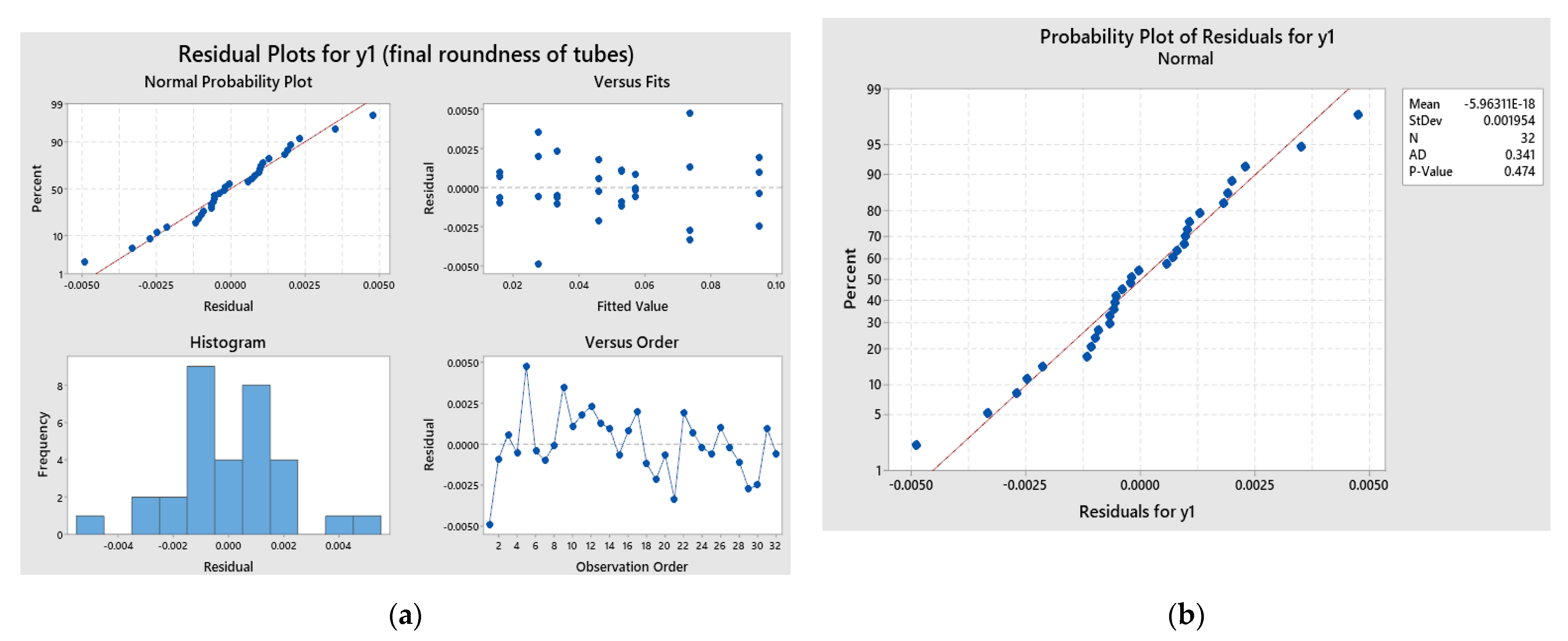
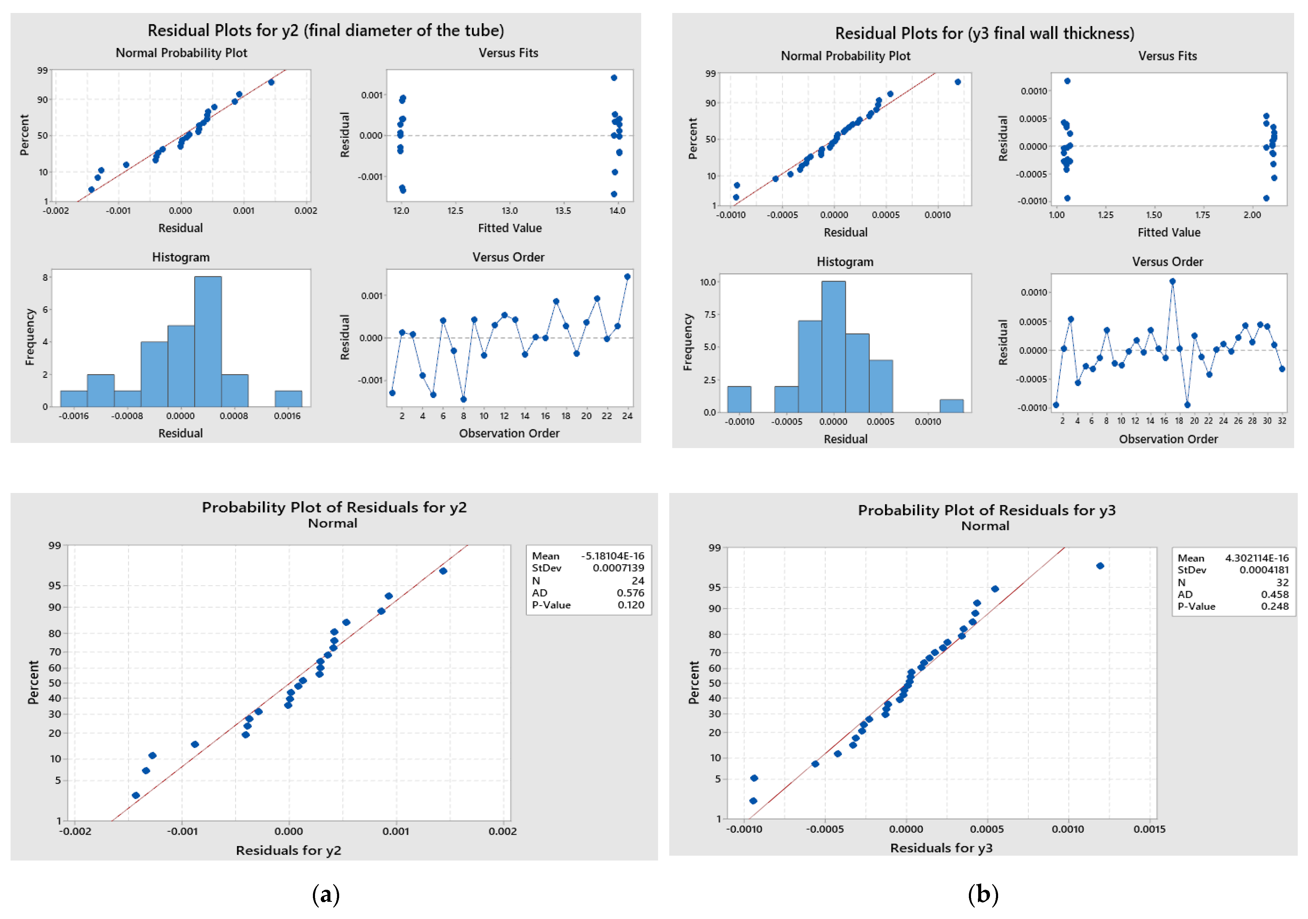
Given the size of the experimentation in this paper, the fulfillment of such assumptions is detailed using only one of the response variables analyzed in the factorial designs, e.g., y₁ (see Figure 6a,b). A similar process of analysis applies for the rest of the variables, and, in consequence, the authors only graphically present the results of the verification of the assumptions for them without further explanation (see Figure 7).

From the previous Figure 6a, it is possible to see that the normal probability plot exhibits a very good fit to the straight line, and there is no relevant outliers that may affect the subsequent ANOVA. Further, if also taking into account that the sample plotted is not small in size, then it is possible to say the residuals are normally distributed. This previous statement is also confirmed if looking at the results of the Anderson–Darling test for normality shown in Figure 6b.

Similarly, the residual versus fit plot indicates that there is not any obvious pattern or structure, because it shows a random order of residuals on both sides of the center line, which confirms that the homoscedasticity assumption is also fulfilled, or that there is no reason to suspect any violation of it.

As for the histogram of the residuals, it shows the distribution of the residuals for all observations given that it is an exploratory tool to prove the general characteristics of these data. In this particular case, it is also possible to confirm that the data are not skewed, and there are no outliers, which is extremely important when working with factorial designs and ANOVA. This histogram supports what was already confirmed with the normal probability plot.

The last plot refers to the residuals versus the order of the data. In this case, the plot shows no trends, patterns, or shifts, and it is possible to appreciate the residuals are randomly located around the center line. In consequence, the authors can assume the residuals are uncorrelated with each other, or that they are independently distributed, which is another ordinary least squares assumption met by the data under question.

Once it was verified that all the ordinary least squares assumptions had been met, it was possible to continue with the ANOVA for all of the studied variables. For these purposes, the software Minitab, version 19, was selected and used. A summary of the key statistics and values of the ANOVA results is shown in

Table 11. Summary of key ANOVA values for the response variables y₁ and y₂.

	y1 (Final Roundness of the Tube)			y2 (Final Outer Diameter of the Tube)
Source	MS	F	p-Value	MS	F	p-Value
Diameter of the pre-tube (A)	3.295 × 10−3	6.684 × 102	p < 0.001 × 10−13; p → 0	5.125 × 10−7	0.70	0.415
Wall thickness (B)	4.675 × 10−3	9.485 × 102	p < 0.001 × 10−13; p → 0	5.823 × 10−3	7.948 × 103	p < 0.001 × 10−13; p → 0
Diameter of the die (C)	2.796 × 10−3	5.673 × 102	p < 0.001 × 10−13; p → 0	2.397 × 10−1	3.272 × 107	p < 0.001 × 10−13; p → 0
A * B	4.445 × 10−3	9.017 × 102	p < 0.001 × 10−13; p → 0	4.532 × 10−5	6.187 × 101	0.069 × 10−5; p → 0
A * C	1.239 × 10−3	2.514 × 102	p < 0.001 × 10−13; p → 0	2.810 × 10−4	3.836 × 102	0.013 × 10−5; p → 0
B * C	1.622 × 10−3	0.329 × 102	0.0653 × 10−4; p → 0	1.014 × 10−3	1.384 × 103	p < 0.001 × 10−13; p → 0
A * B * C	1.686 × 10−3	3.421 × 102	p < 0.001 × 10−13; p → 0	1.801 × 10−5	2.459 × 101	0.014 × 10−2; p → 0
Error	4.930 × 10−6			7.325 × 10−7

and

Table 12. Summary of key ANOVA values for the response variable y₃.

	y3 (Final Wall Thickness of the Tube)
Source	MS	F	p-Value
Diameter of the pre-tube (A)	1.084 × 10−5	4.802 × 101	0.036 × 10−5
Wall thickness (B)	0.879 × 10−1	3.891 × 107	0.00000
Diameter of the die (C)	2.183 × 10−3	9.666 × 103	0.00000
A * B	2.348 × 10−3	1.040 × 104	0.00000
A * C	8.972 × 10−4	3.973 × 103	0.00000
B * C	1.869 × 10−4	8.274 × 102	0.00000
A * B * C	6.187 × 10−4	2.739 × 103	0.00000
Error	2.258 × 10−7

.

Based on the p-values from the previous Table 11 and Table 12, and also on the Pareto graphs related to each of the ANOVAs, the authors of this paper can conclude that there are many significant terms affecting the behavior of the response variables under study.

In the particular case of the variable y₁, or the final roundness of the tube, there is a clear and total significance of all the factors and their interactions over its results, meaning that they are active, with a confidence level of 95%, and there is thus significant statistical proof for the rejection of their respective null hypotheses. In practical terms, this means that during the cold tube drawing process under study, the use of different pre-tube diameters, pre-tube wall thicknesses, and die diameters and their combinations has an important effect on the results of the roundness. After a profound analysis of the outcomes among the authors of the paper and with experts from the industrial sector, it was possible to unanimously come to the conclusion that these results and their significance can also be explained by a few other elements such as the technological precedence of the elements involved (technological heritage or simply how the tubes or even dies have been produced before). Another important element explaining the statistical significance refers to the nature of the cold tube drawing process carried out for the purposes of this paper (single-pass) and the size of reductions which are significant for a drawing of this type. In this sense, it is recommended to, among other things, first make sure that the pre-tubes and the die have highly precise dimensions and zero defects in order to obtain the best possible roundness results, or at least not to increase their effect over the variable. It is also advisable to maintain a tight control over the lubrication of the die given that it is also an element that can influence the results of the variable y₁.

On the other hand, in the case of the variable y₂, or the final outer diameter of the tube, it is possible to appreciate that, except for factor A, or the diameter of the pre-tube, most terms are also highly significant and affect this variable to a great extent. In all cases where the p-value yielded a value less than 0.05, it is possible to conclude with a confidence level of 95% that the null hypotheses for these terms were rejected. In practical terms, this means that the isolated effect of factor A does not significantly affect the dimensions of the final tube. As for the remaining factors and their interactions, such significance can be explained by elements such as the above-mentioned technological precedence of the elements involved or the nature of the cold tube drawing process carried out for the purposes of this paper (single-pass), and the subsequent large size of reductions that took place in the experiment. Likewise, checking for zero defects and precision dimensioning in the pre-tubes and dies is also of vital importance in order not to further increase the significance of the active factors and their interactions.

Finally, in the case of the third response variable y₃, or the final wall thickness of the tube, it is also possible to see that, as for the case of y₁, all the terms significantly affect the final values of it, and thus this translates into the need to carefully respect the quality standards and dimensions of all factors involved in order to achieve the most accurate wall thickness in the resulting tubes after the drawing process. Of special importance is the die used, as well as its proper lubrication; according to the experience of the authors and the consulted experts, this is an important factor influencing the final results of this variable.

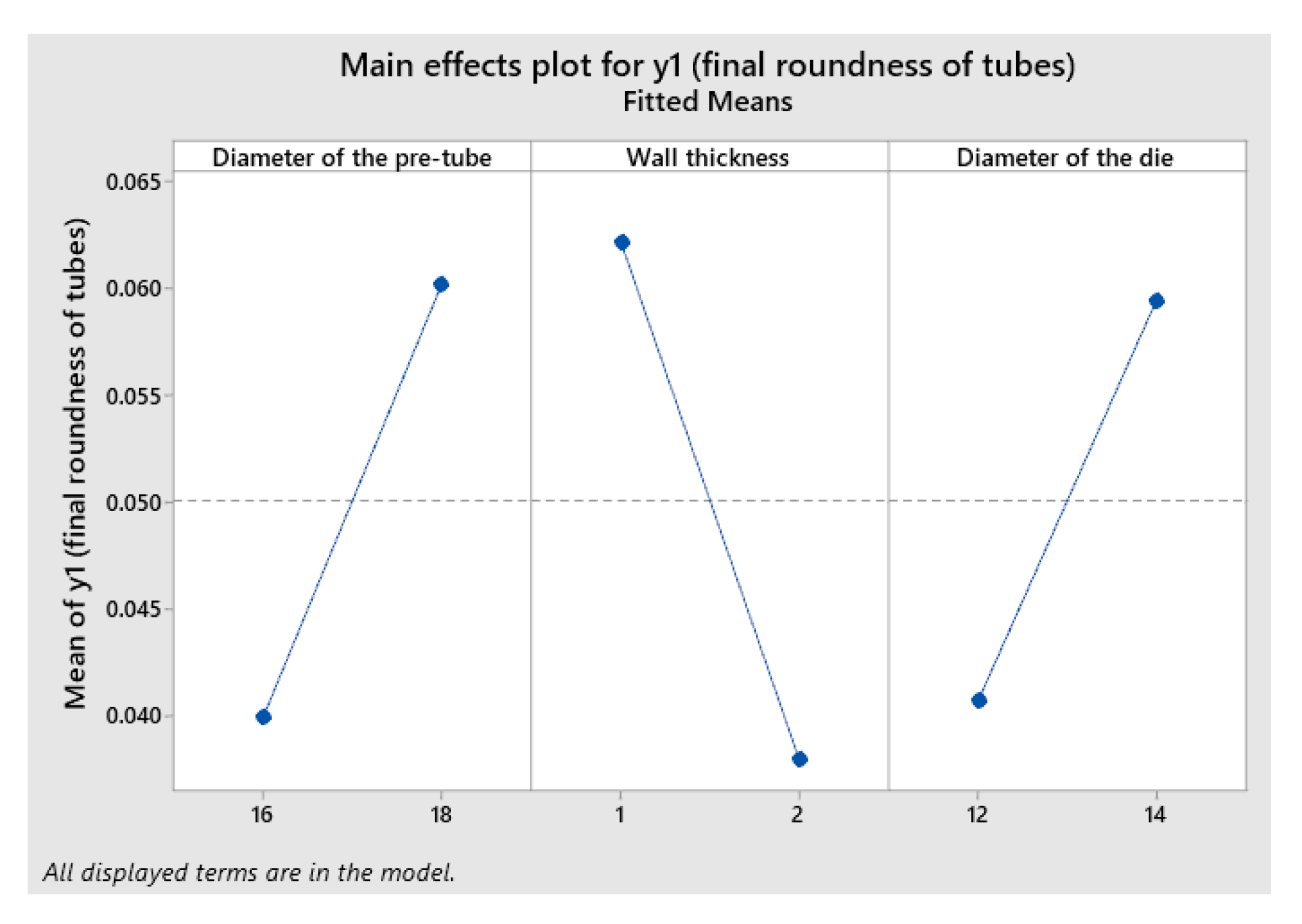
The following Figure 8 presents the plot for all main effects. The analysis of these graphs also helps in interpreting and/or contributing to the understanding of a key part of the results obtained with the ANOVA, and specifically the impact of the main terms involved on the studied variables. As mentioned before, given the size of the experimentation in this paper, the graphs are only presented for the case of the response variable y₁, or the final roundness of the tube; however, a similar process of analysis indeed applies for the rest of the variables, and readers and reviewers of this paper are welcome to request access to these extra graphs if needed.

From this figure, it is possible to see that there are main effects present in the case of all factors, leading the authors to confirm that the response mean is not the same across all of the factor levels. In more concrete terms, it is possible to see that the lower level of the diameter of the pre-tube (factor A) has the lowest effect on the response variable y₁, or the final roundness of the tube, while its upper value behaves in the opposite manner. A similar analysis applies for the diameter of the die (factor C), while in the case of the remaining factor (factor B), its lower value influences the response variable the most. All of these analyses closely relate to those in Table 11, where it can be seen that the interactions of all these factors are significant as well.

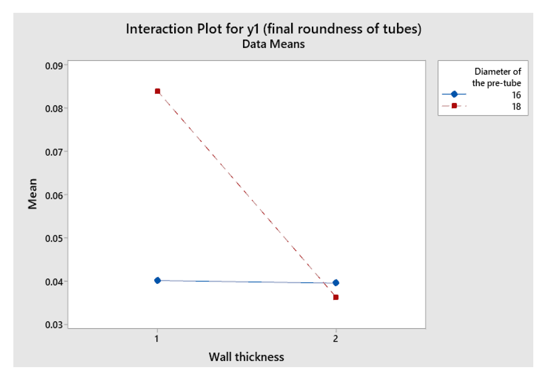
Another tool the authors decided to use for a better analysis of the results and data was the interaction plots. These plots allowed viewing and/or reaffirming how a given categorical factor and a continuous response depend on the value of the second categorical factor. Given the many pages that would be needed within the paper to show all of the interaction plots analyzed, the authors show an illustrative example of the interaction plot for y₁ considering the factors “diameter of the pre-tube” and “wall thickness of the tube”. As it can be appreciated in Figure 9, there is a lack of parallelism between both lines, which reaffirms the effects manifested by the respective p-value in Table 11. This, in practical terms, means that the relationship between the response variable y₁ and the wall thickness also depends on the diameter of the pre-tube. Conclusions such as this are extremely important in the context of the specific cold tube drawing process under study and represent valuable information for either research teams or the end user of this research. Once more, the readers and reviewers of this paper are kindly invited to ask for any other proof of these results in case they find it necessary.

4. Conclusions

This paper presented an experiment associated with the cold tube drawing process, which is of tremendous importance for industry, especially in today´s manufacturing-driven Europe. The authors wanted to investigate the potential relation and influence of three relevant factors: A (diameter of the pre-tube), B (wall thickness of the pre-tube), and C (diameter of the die), and their interactions over the defining response variables, i.e., y₁ (final roundness of the tube), y₂ (final outer diameter of the tube), and y₃ (final wall thickness of the tube). The selection of these factors, their levels, and the response variables was based on the authors´ experiences, but mainly on the manifested interests and needs of key European tube manufacturers given these types of tubes’ significant presence or high volumes in the production process, and their subsequent significant use as parts and components in many other manufacturing processes, with emphasis on the automotive industry. In this paper, the authors also wanted to see how these factors behaved under the conditions of a single-pass tube drawing process in order to also investigate its efficacy as an alternative to more costly and time-consuming double- or multi-pass approaches, a problem that has been affecting the tube manufacturing industry for decades. The physical part of the experiment was realized on specimens of pre-tubes with diameters of ø16 and Ø18 mm, whose initial wall thicknesses were 1 and 2 mm, drawn using dies of Ø12 and Ø14 mm. The equipment related to the drawing process consisted of a hydraulic tensile testing machine, EU 40, with a clamping fixture, as shown, in detail, in Figure 2 and Figure 3.

In order to carry out the investigation, the authors implemented a factorial design of experiments of the 2³ type, given its many advantages for screening purposes and, to an extent, its superiority over other designs such as the 3^k type. The combinations and details of the experiment are presented in Table 5, Table 6, Table 7 and Table 8, and the number of measurements or runs was 32, 32, and 24 for the variables y₁, y₂, and y₃, respectively. As a complement to the realization of the experiment, the authors also wanted to offer a methodological take on the approach, and thus they also presented in this paper: 1. General Guidelines for Designing an Experiment, and 2. An Analysis Procedure for a 2^k Design. Both methodological tools were based on previous publications on the issue; however, they also add some methodological value and value of use to the content presented in this research.

The measurement of the response variables took place on a CMM, ZEISS CenterMax, at room temperatures between 25 and 27 °C, as shown in Figure 5. Given the time and financial resources available, four, four, and three replicates associated with the above-mentioned runs for y₁, y₂, and y₃, respectively, were executed on this machine, which clearly explains the number of runs mentioned before and fulfills, in any case, the requirements for an experiment of this type, as mentioned in the introduction and covered in detail by authors such as [20,26].

The obtained data were subsequently processed by the statistical software Minitab 19. The first step in the software was to verify that all DOE-related ordinary least squares assumptions were met. Subsequently, the ANOVA results obtained offered clear proof that the vast majority of the factors and their interactions were significant at the 95% level of confidence, thus justifying the rejection of the associated null hypotheses.

After a careful analysis and consideration of the results, the authors established a series of findings where they all agreed that it was of vital importance to ensure high standards of quality and precision levels were being met for the factors under study. This was found to be vital in order to avoid any influence or effect related to the technological precedence of the elements involved (technological heritage or simply how the tubes or even dies had been produced before). This conclusion was of special importance for the case of the die because in the cold tube drawing process, the resulting diameter of the tubes, their wall thickness, and even their roundness itself, i.e., variables y₂, y₃, and y₁, respectively, highly depend on the die´s condition and, as mentioned before, on its precise dimensioning as well. In this regard, the authors also concluded that it was necessary to keep a tight control over the lubrication of the die given the proven potential for it to be statistically and technologically significant in all response variables under study.

Another important finding explaining the significance of the factors and their interactions was linked to the single-pass nature of the cold tube drawing process investigated in this paper. This type of approach implied large size reductions, which proved to be significant for the drawing of the tubes, which would otherwise have been realized through a double- or multi-pass approach, a process that, even though it is more time consuming and expensive, usually offers less deviations from the product geometrical specifications.

All these conclusions open several more questions to be answered in future research by the authors of this research, while at the same time, they clearly answer the initial question of whether, under the circumstances and factors defined for this research, the single-pass cold tube drawing process is a viable alternative to more expensive and time-consuming multi-pass processes.

Further research will focus on analyzing these same factors under the single-pass approach, but also taking into account the recommendations and precautions mentioned above. It is also a goal of the authors to replicate what was conducted in this research under a multi-pass approach in order to compare and set clearly quantifiable differences between both courses of action. At the same time, further research will also cover the analysis of these factors in relation to other relevant response variables that are problematic for industrial practice and science.