A Data-Driven Model of Cable Insulation Defect Based on Convolutional Neural Networks

Abstract

The insulation condition of cables has been the focus of research in power systems. To address the problem that the electric field is not easily measured under the operating condition of 10 kV transmission cables with insulation defects, this paper proposes a data-driven cable insulation defect model based on a convolutional neural network approach. The electric field data during cable operation is obtained by finite element calculation, and a multi-dimensional input feature quantity and a data set with the electric field strength as the output feature quantity are constructed. A convolutional neural network algorithm is applied to construct a cable data-driven model. The model is used to construct a cloud map of the electric field distribution during cable operation. Comparing the results with the finite element method, the overall accuracy of the data-driven model is 94.3% and the calculation time of the data-driven model is 0.025 s, which is 360 times faster than the finite element calculation. The results show that the data-driven model can quickly construct the electric field distribution under cable insulation defects, laying the foundation for a digital twin structure for cables.

1. Introduction

With the continuous development of power grid technology, the use of power cables is rapidly increasing and their coverage is becoming larger and larger. The operation and then reliability of power cables directly affects the safe and stable operation of the power system. Small defects in the cable during manufacture or installation can be excited by over-voltage ageing, temperature, microorganisms and other factors. If the cable is not de-contaminated and treated in a timely manner, it will lead to cable failure and bring great losses to production and life [1]. The traditional study of cable insulation impurity conditions consists of two main methods: physical experiments [2] and theoretical calculations [3]. Most physical experiments on cable insulation are preventive tests, i.e., measuring insulation resistance [4], DC withstand voltage [5] and leakage current [6], which do not allow for the assessment of the insulation condition during cable operation. Currently, finite element modelling calculations are also used in some studies to assess the state of cable insulation in the presence of impurities [7]. In the literature [8], the electric field distribution of cables during normal operation was calculated by modelling with the finite element method. Reference [9] calculated the electric field distribution in the case of cable defects (including impurities) by using finite element calculation software. The method of finite element modelling calculations has significant advantages in terms of cost and cycle time of the study. The accuracy and reproducibility of the results are good [10], which is of practical interest for observing the electric field distribution of cable insulation under different operating conditions. However, there are still limitations to the finite element calculation method. Due to the complexity of cable operating conditions, finite element models of cables are often complex and take relatively long to calculate [11]. Therefore, it is difficult to study the electric field in the case of impurities in the cable insulation using the finite element method alone.

Convolutional neural networks (CNN) evolved from the structure of the biological visual system to obtain specific features and recognize the corresponding patterns in graphic images [12]. Convolutional neural networks are widely used because of their characteristics of local perception and weight sharing, which greatly reduces the number of training parameters and improves the computational efficiency of complex networks [13]. Compared to other deep learning methods, CNN algorithms are much less complex and challenging to train, reducing the risk of overfitting [14]. It is relatively easy to build networks with deep structure using CNN algorithms.

Machine learning has been successfully applied in many fields and is increasingly being used in the power industry [15]. The literature [16] uses neural networks to evaluate the insulation conditions of 11 kV paper cables. The literature [17] identifies cable partial discharge defects by means of different neural network models and the literature [18] uses fuzzy neural networks to evaluate cable insulation. The literature [19] identifies the partial discharge signals of cables by means of a data-driven model. These studies all classify and identify cable faults and the results of the data are generally one-dimensional. In this paper, the data-driven model is used to achieve the prediction of the electric field distribution of the cable operating condition, presenting a two-dimensional distribution cloud of the cable electric field. Finite element calculations provide the underlying data, which is then learned through artificial intelligence methods to construct a data-driven model of the electric field in the case of cable defects. The research in this paper is based on this idea. The electric field data of the cable is obtained through finite element calculations, and a CNN-based data-driven model is constructed from the multidimensional input feature quantities of the cable. Finally, the calculated values of the data-driven model are post-processed to draw a cloud map of the electric field intensity distribution of the cable. The rest of this paper is as follows: Section 2 introduces the principles of finite element calculations, constructs a finite element model of the electric field of the cable and sets the boundary conditions of the model. Section 3 describes the data-driven model of the electric field of the cable, including the selection of the feature variables, the comparison of algorithms, the selection of parameters for the convolutional neural network and the process of constructing the prediction model. Section 4 evaluates the prediction model and analyses the results. Finally, conclusions are drawn in Section 5. The research in this paper combines artificial intelligence algorithms with finite element calculation models to compensate for the disadvantages of complex finite element calculation models with long computation times, and to visualize the electric field distribution of the cable operation. The method can also be applied to the digital twin research process.

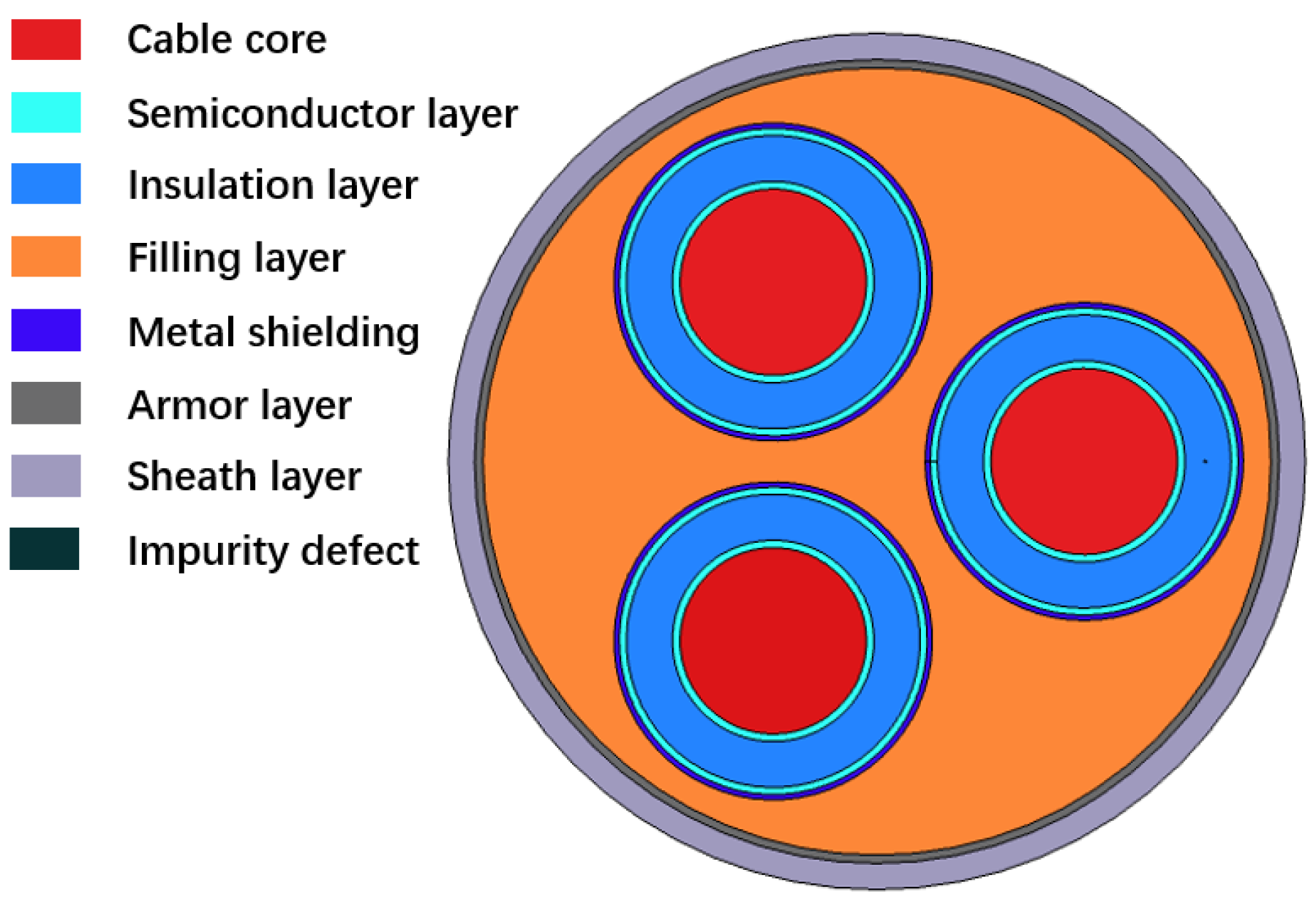
2. Finite Element Modeling Method of Cable

A cross-linked polyethylene (XLPE) three-core cable of 10 kV commonly used in the model YJV22-8.7/10-3 × 240 mm² was chosen as the object of finite element calculations. The cable model containing impurities was constructed by the finite element calculation software COMSOL Multiphysics and the cable model was constructed as shown in Figure 1.

The core, semiconductor layer, insulation layer, shielding layer, filler, armor layer and outer sheath of the three-phase axisymmetric cable are set. The geometric parameters of each structure of the cable are shown in

Table 1. Geometric parameters of cable structure.

Structure	Materials	Inner Diameter/mm	Outer Diameter/mm
Cable cores	Copper	11.9	11.9
Conductor shielding	Semiconductor Materials	11.9	12.7
Insulation layer	XLPE	12.7	17.2
Shielding layer	Copper	17.2	17.3
Cable three-phase filler	Polypropylene	41.1	41.1
Armor layer	Aluminum	41.1	41.11
Outer sheath	Polyethylene	41.11	43.11

.

After constructing the model using COMSOL Multiphysics finite element calculation software, the control equations involved are analyzed. This paper is a study of the cable electric field under steady state conditions, so the set of equations involved is as follows.

$$\mathit{E}=-\nabla \phi$$

(1)

$$\nabla \cdot \mathit{D}=\rho$$

(2)

$$\nabla \cdot \mathit{J}=-j\omega \rho$$

(3)

In the above equation, $\mathit{E}$, $\mathit{D}$ and $\mathit{J}$ are electric field strength, potential shift vector and current density. $\phi$ is electric potential, $\rho$ is charge density.

The constitutive relationship of the material properties is

$$\mathit{D}=\epsilon \mathit{E}$$

(4)

$$\mathit{J}=\sigma \mathit{E}$$

(5)

where, $\epsilon$ is relative electric permittivity, $\sigma$ is electrical conductivity.

Based on Equations (1)–(5), the differential equation for $\phi$ is obtained as follows.

$$\nabla \cdot \left(\left(\sigma +j\omega \epsilon \right)\nabla \phi \right)=0$$

(6)

After choosing the control equations for the model, the boundary conditions for the model are then determined.

In a three-phase AC cable, the phase difference between the voltages of the three phases A, B and C is 120 degrees. The A-phase voltage ${\phi }_a$, B-phase voltage ${\phi }_b$, and C-phase voltage ${\phi }_c$ are set as follows.

$$\begin{gathered} {\phi }_a={\phi }_0{e}^{j0} \\ {\phi }_b={\phi }_0{e}^{-j\frac{2\pi }{3}} \\ {\phi }_c={\phi }_0{e}^{+j\frac{2\pi }{3}} \end{gathered}$$

(7)

After determining the boundary conditions, the finite element model is meshed and then the finite element calculations are performed on the model.

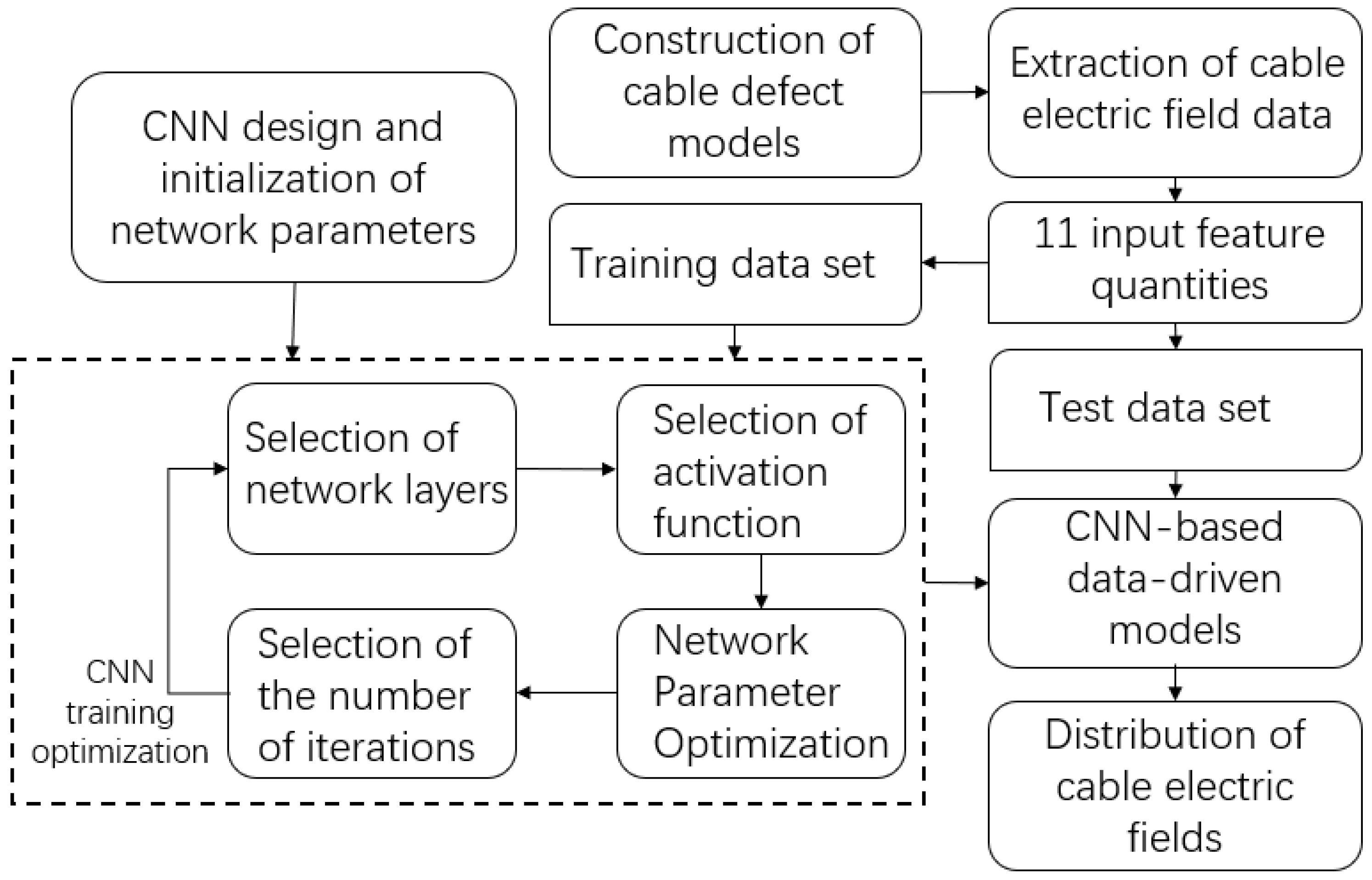
3. Modeling Method of Data-Driven Model

3.1. Data Set Construction of Data-Driven Model

In the finite element calculation, the most obvious reflection of the impurities in the cable insulation should be the electric field strength. The uneven variation of the electric field strength at the impurities reflects the influence of the impurities on the interior of the insulation. At the same time, the electric field strength can also be used as the basic data to reflect whether the insulation is broken down or not. The variation of electric field strength is also the fundamental variable of most concern in cable insulation. In the algorithmic learning of convolutional neural networks, if there is a relatively strong correlation between several input feature quantities, the learning results will automatically filter the feature quantities. Therefore, when selecting the input feature quantities, the description of the constructed model needs to be comprehensive enough. In this paper, data related to the structure of the cable, the operating parameters of the cable, and the structural parameters of the impurities are used as input feature values to construct a data set consisting of multidimensional vectors, and the 11 input feature quantities are selected as shown in

Table 2. Input feature quantities.

Number	Input Feature Quantity
1	Cable core radius
2	Thickness of insulation layer
3	Cable operating voltage
4	Number of impurities
5	Relative electric permittivity of impurities
6	Electrical conductivity of impurities
7	Relative electric permittivity of the insulation layer
8	Electrical conductivity of the insulation layer
9	X coordinate of the fetching point
10	Y coordinate of the fetching point
11	Cable operating frequency

. Among them, the dimensions of the cable are represented by a right-angle coordinate system. The data were extracted from 12 different locations selected from different locations of the cable, constituting a data set of approximately 2.12 million groups.

3.2. Data-Driven Model Implementation Based on CNN

The convolutional neural network is a neural network algorithm based on convolutional operations with a parameter sharing mechanism and a deep structure. The essence of a CNN is a mathematical model that maps the original input to a new feature representation through multiple layers of data transformation and dimensionality reduction. The number of layers, the size of the convolutional kernel, the non-linear activation function and the pooling method are some of the main aspects that affect the prediction accuracy of a convolutional neural network model.

Before building a data-driven model, the first step is to choose the algorithm for training the model. The basic structure of a convolutional neural network consists of an input layer, a convolutional layer, a pooling layer, a fully connected layer and an output layer. Several convolutional and pooling layers are generally taken, using an alternating setup of convolutional and pooling layers, i.e., one convolutional layer is connected to a pooling layer, another convolutional layer is connected after the pooling layer, and so on. The convolutional layer adopts a weight-sharing technique, using a series of convolutional kernels to map local features at low levels to global features at high levels, which can significantly reduce the network parameters and improve the computational efficiency, avoiding the overfitting phenomenon. The pooling layer is usually used immediately after a convolutional layer, whose purpose is to reduce the feature dimension and highlight the main features. The specific convolution calculation formula is as follows [20].

$$h\left[i,j,\tau \right]={{\displaystyle \sum }}_m{{\displaystyle \sum }}_{n}X\left[i+m,j+n,\tau \left]K\right[m,n,\tau \right]+b_{\tau }=X\otimes K+b_{\tau }$$

(8)

In the above equation, the length $m$, width $n$ and depth $\tau$ of the convolution kernel are first selected. $\tau$ is also the number of convolution kernels. Then the input data is converted into the input matrix $X$ and substituted into the convolution calculation formula. The output matrix $h$ is obtained, where $i,j$ and $\tau$ represent the three dimensions of the output matrix respectively. $b_{\tau }$ is the threshold of the $\tau$th convolution kernel. $\otimes$ denotes the product of the corresponding elements of the matrix multiplied together.

Like neural networks with conventional structures, the optimization objective of convolutional neural networks is to minimize the loss function to find the optimal parameters. In this paper, we use the mean square error (MSE) loss function as the objective function. the MSE function is represented by Equation (9)

$$L_{ossmse}=\frac{1}{N}{{\displaystyle \sum }}_{i=1}^N{(y_i-f\left(x_i\right))}^2$$

(9)

In the above equation: $N$ is the number of samples; $y_i$ and $f\left(x_i\right)$ are the expected and actual outputs of the model, where they represent the actual and predicted values of power, respectively.

The essence of convolutional neural networks is that each convolutional layer contains a certain number of eigenfaces or convolutional kernels. Compared with traditional fully connected networks, convolutional neural networks in which the weights of the convolutional layers are shared use the network to reduce the number of training parameters, reducing the complexity of the network model, reducing overfitting, resulting in better generalization capabilities, and operating with fewer connections and parameters than traditional fully connected networks, making them easier to train. In addition, convolutional neural network systems use shared parameters of connection weights in the same convolutional or pooling layers. These features greatly reduce the number of parameters and reduce the complexity of data training and the risk of training overfitting. Consequently, convolutional neural networks offer significant advantages and powerful feature learning capabilities in building deep structural neural networks [21]. As the number of layers increases, the feature extraction of the convolutional neural network gradually increases, but the number of parameters needed for training also needs to increase, so the demand for sample data also increases, which may also make the sample data will be over-fitted [22]. However, there is no mature theoretical framework for the determination of the number of network layers. Therefore, in the actual training process, the optimal structural system needs to be selected through a large number of experiments in order to choose a better performance.

3.3. Data-Driven Model Implementation Based on CNN

This section evaluates the classification performance of convolutional neural networks, examining the effects of different network layers, different activation functions and different pooling methods on cable data-driven models, and comparing them with back propagation neural network (BPNN).

The performance of a convolutional neural network is highly dependent on the number of layers in the network. In this paper, we tested the performance of 1–5 layers of convolutional neural network respectively, using the pooling method of maximum pooling, the activation function using Swish function, the number of convolutional kernels of each layer are 32, and the size of convolutional kernels are all 3 × 3. The results are shown in

Table 3. Computational accuracy of CNN with different number of layers.

Number of Network Layers	Accuracy/%
1	89.3
2	93.2
3	95.8
4	93.2
5	91.3

.

When the number of layers of the network is reduced, the ability of the convolutional neural network to fit the samples will be reduced. When the number of layers is too large, although the network can extract deeper data features, the information transfer between the layers of the network will cause data wastage and overfitting problems, instead making the training accuracy decrease and the training time increase. As can be seen from Table 3, convolutional neural networks work better at 3 layers. The two mainstream pooling methods are maximum pooling and average pooling, and the maximum pooling method has better recognition accuracy than average pooling because it can extract the most characterizing features. Therefore, the final convolutional neural network architecture used in this paper consists of three convolutional layers and three pooling layers.

In addition, the performance of convolutional neural networks was compared with BPNN, and the results are shown in

Table 4. Comparison of the computational accuracy of CNN and BPNN.

Cable Operating Parameters	Accuracy/%
	CNN	BPNN
Cable core voltage	95.8	94.6
Impurity conductivity	94.6	94.2
Operating frequency	92.6	92.6
Overall accuracy	94.3	93.8

.

As can be seen from Table 4, the overall accuracy of the convolutional neural network in both methods reached 94.3%, which is higher than the computational accuracy of BPNN.

The process of building a data-driven model based on convolutional neural networks is shown in Figure 2. Firstly, the original data is collected on the distribution of electric field under different operating conditions of the cable, and 11 feature parameters affecting the cable operating condition are constructed to obtain the cable feature dataset. The feature data set is then divided into a training set and a test set, with 80% and 20% of the weight of each respectively. The optimized convolutional neural network algorithm was trained by using a small-batch stochastic gradient descent algorithm [23] on the training set to minimize the error between the predicted and actual outputs of the model, and the performance of the model was evaluated by the test set.

4. Results and Discussion

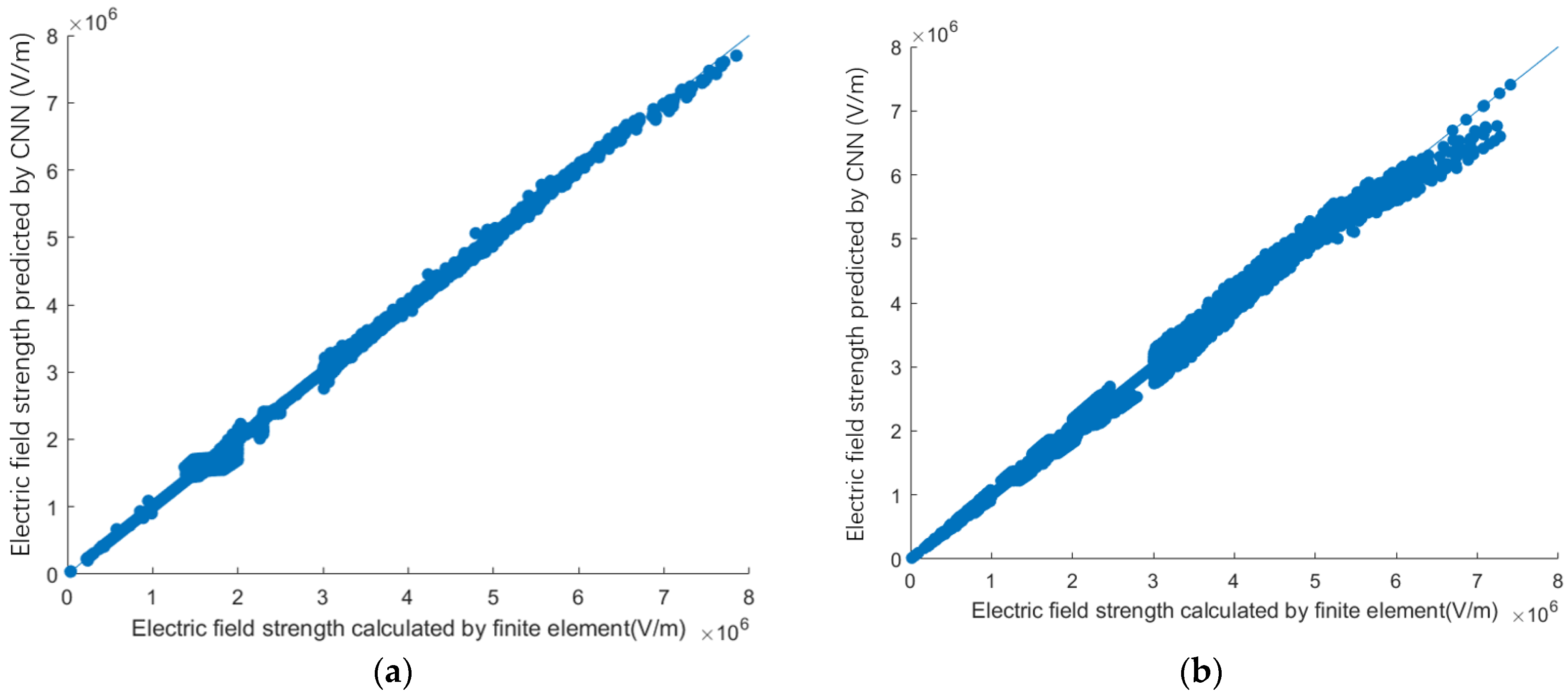
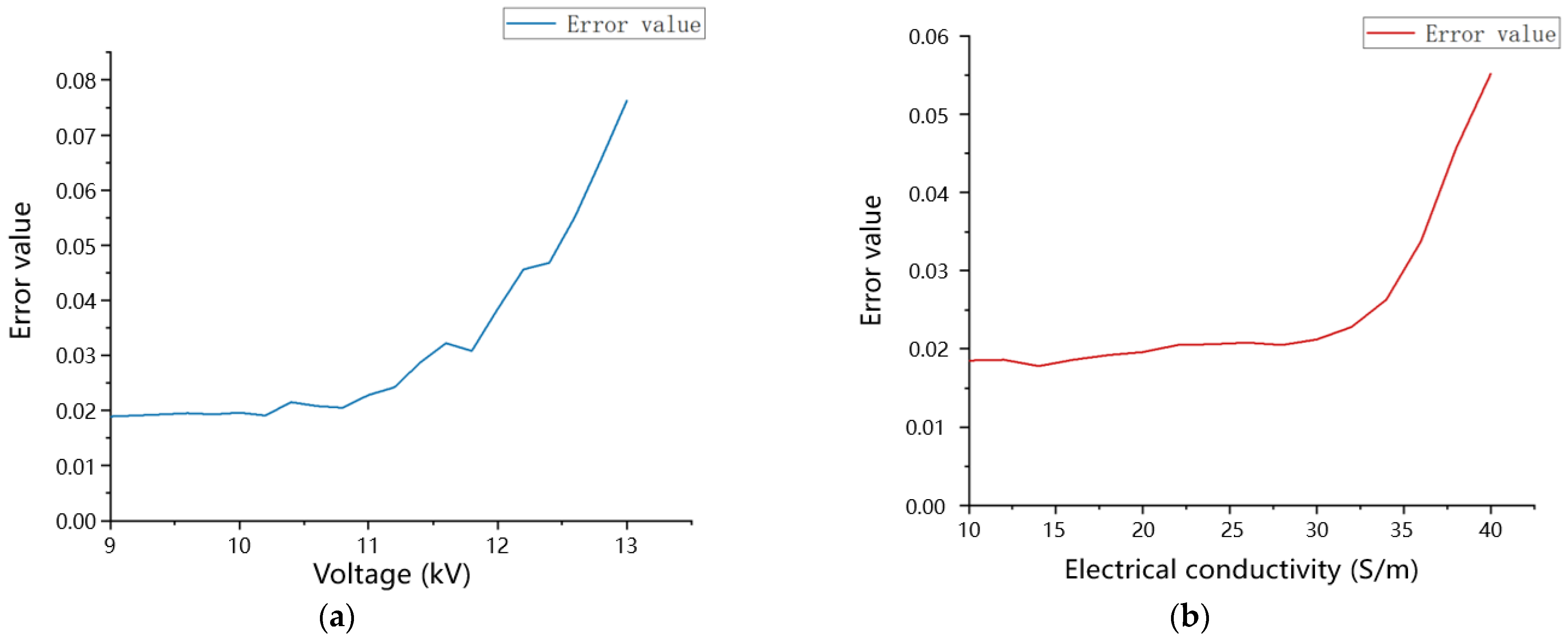
4.1. Accuracy Analysis of Data-Driven Models

The original data set is divided into a training set and a test set. After generating a model by learning the data in the training set, the data in the test set is predicted to verify the accuracy of the model. The model’s accuracy is expressed by the accuracy, and the accuracy r is calculated as shown in Equation (10).

$$r=\sqrt{1-m/n}$$

(10)

In the above equation: $m$ is the sum of the squares of the actual and predicted values, $m=\sum {\left(l_{true}-l_{predict}\right)}^2$; where $l_{true}$ is the true value; $l_{predict}$ is the predicted value; and $n$ is the sum of the squares of the differences between the true and predicted values.

By varying the cable operating voltage of the cable model, the accuracy r of the convolutional neural network learning model training set and test set for the electric field strength of the cable was 0.971 and 0.967 respectively. The electric field intensity values calculated by the learning model based on the convolutional neural network algorithm for the single and multiple impurity cases were compared with those calculated by finite elements and the results are shown in Figure 3. Where the x-axis is the electric field strength value calculated by the finite element and the y-axis is the value calculated by the convolutional neural network learning model. As can be seen by the graph below, the learning model fits the data in this case better than the finite element calculated data. However, it can also be seen that there are some points with large deviations in the prediction results. This situation may be caused by the regression principle of the convolutional neural network because the nonlinearity of the electric field intensity near the impurity points is stronger, and the stronger the nonlinearity of the data, the worse the learning effect of the neural network method in the case of insufficient data information. Generally speaking, expanding the dimensionality of the input feature quantity to include more influencing factors can make the judgment more accurate and further improve the prediction accuracy of the prediction model.

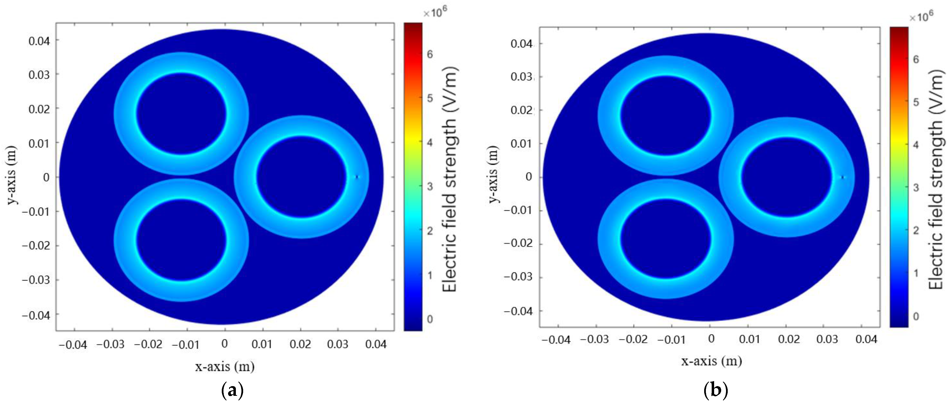
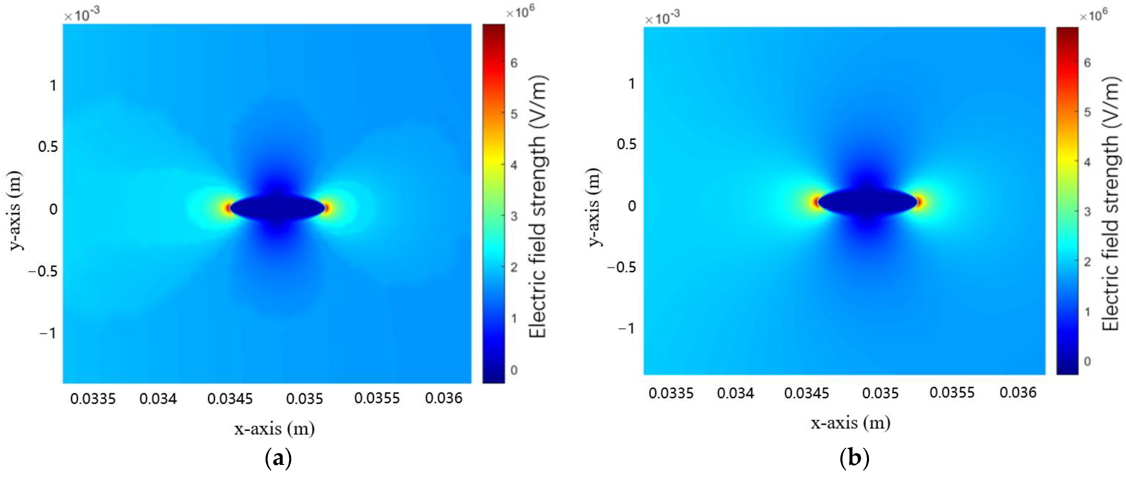
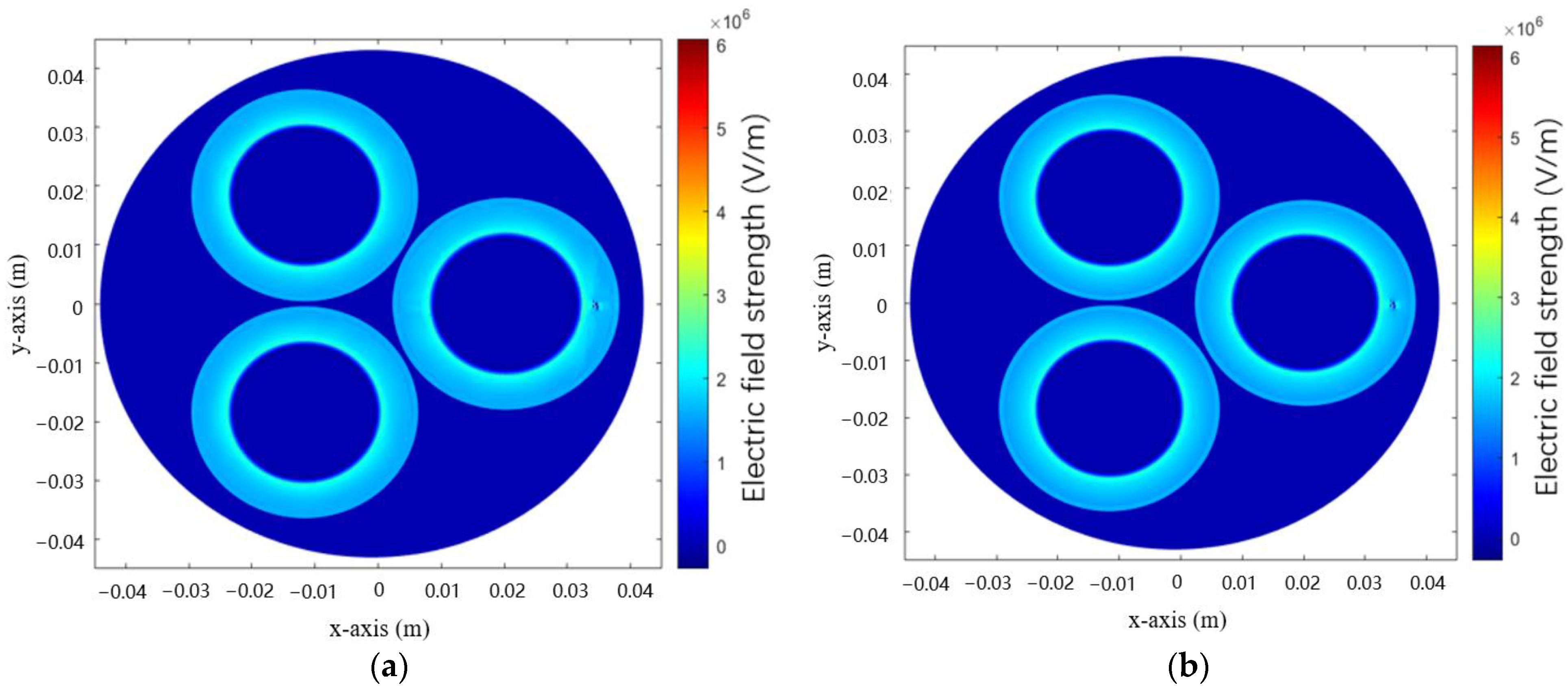
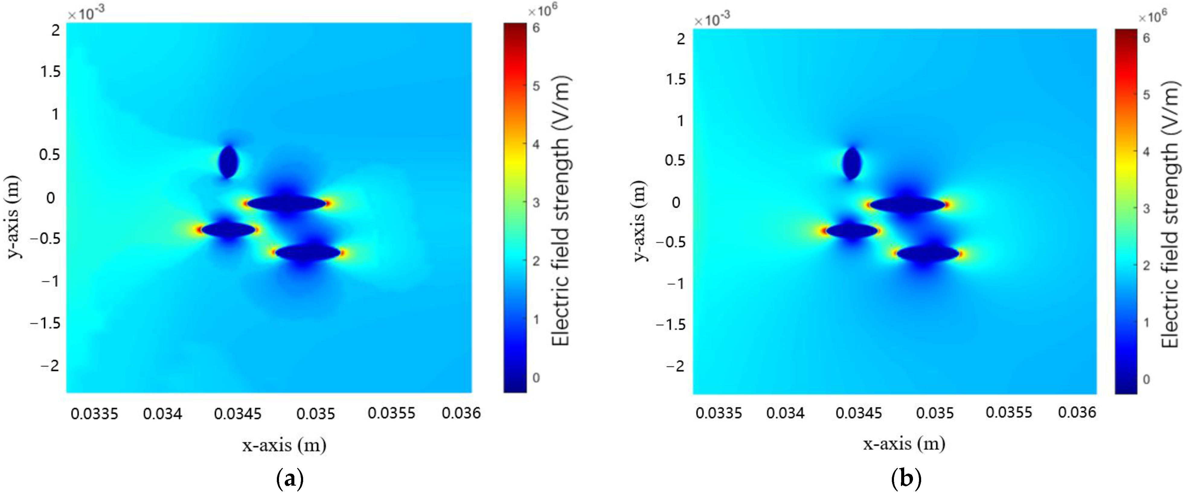
4.2. Predicted Electric Field Strength of the Cable

After applying the convolutional neural network method to learn the data set, a data-driven model of the cable with insulation impurities is created. In this case, the structural parameters of the cable model remain unchanged, and the voltage of the cable operation is changed. At this time, the cable operating voltage is 11 kV, the relative electric permittivity of impurities is 30, the conductivity is 18 S/m, the relative electric permittivity of insulation layer material is 1.5, the conductivity is 0.25 S/m, and the operating frequency is 50 Hz. The electric field intensity at each location of the cable was calculated using the data-driven model, and the electric field distribution clouds were plotted by MATLAB software and compared with those calculated and plotted by COMSOL Multiphysics with MATLAB software, and the results are shown in Figure 4 and Figure 5.

But in practice, the cable insulation layer at the distribution of many impurities, so in the model, other conditions remain unchanged, for multiple impurities in the case of cable operating voltage changes, the electric field distribution of the cable to learn. At this time, the other parameters of the cable remain unchanged, and only the number of impurities and the cable operating voltage are changed. Using the model to predict the electric field strength at each location of the cable, draw the electric field strength distribution cloud map and finite element calculation for comparison, the results are shown in Figure 6 and Figure 7.

The results of the electric field strength calculated by the data-driven model obtained by the convolutional neural network-based algorithm are reliable. Therefore, the cable insulation under the above conditions can be analyzed based on the cloud diagram. From Figure 4, Figure 5, Figure 6 and Figure 7, it can be seen that the cloud diagram composed of the data obtained by learning and the cloud diagram composed of the actual finite element calculation have basically the same values at each position of the model, so the calculation results based on the convolutional neural network algorithm can be considered valid, and the electric field strength of impurities at the tip of the cable insulation in both cases is about 3 × 10⁶ V/m, which is still less than the Breakdown field strength value, so the cable can still operate normally at this time.

In the application of the data-driven model, a point near the impurities in the cable model was analyzed to examine the error between the values obtained by algorithmic learning within the training set and outside the training set and the finite element calculated values when the cable core voltage and the impurity conductivity were varied respectively, as shown in Figure 8. In this case, the voltage values of 9–11 kV and the conductivity of 10–30 S/m were set as the training set.

From Figure 8, the error between the data-driven model and the finite element calculations increases when the core voltage is greater than 11 kV or the conductivity of the impurities is greater than 30, while the error between the data-driven model and the finite element calculations increases when the core voltage is greater than 11 kV or the conductivity of the impurities is greater than 30. When the calculated core voltage or impurity conductivity is too large, the error in the data-driven model is greater than 5%. As can be seen, the accuracy of the predicted values decreases significantly when the predicted values are far from the data set. It can be seen that the results of the data-driven model for the electric field strength of the cable are in general agreement with the finite element calculations. The accuracy of the data-driven prediction model constructed by the convolutional neural network algorithm can be guaranteed within the range of the actual operation of the cable.

5. Conclusions

(1) This paper proposes a data-driven model based on convolutional neural network to calculate the electric field distribution of cables. After obtaining the basic data through finite element calculation, the convolutional neural network constructs a data-driven model that can replace the finite element calculation to construct the electric field distribution results of the inner insulation of cables containing impurities. By comparing the CNN with the BPNN, the data-driven model constructed by the CNN algorithm has a higher accuracy, with an overall accuracy of 94.3%. The calculation time of the data-driven model is 0.025 s, which is approximately one 360th of the finite element calculation and much less than the finite element computational time required for the calculation.

(2) To address the problem that the model needs to be changed at the same time when the operating parameters of the cable are changed in the finite element calculation. The data-driven model constructed in this paper contains 11 input characteristic quantities related to the actual operating parameters of the cable, so that the electric field distribution of the cable can be calculated directly by the data-driven model when the operating conditions of the cable are changed. The results show that when the cable parameters are in the training set, the error in the electric field distribution calculated by the data-driven model is within 3% when varying the core voltage and the material parameters of the impurities. In the actual working condition, the parameters of the cable in normal operation are included in the training data set of the model.

(3) The data-driven model constructed in this paper based on convolutional neural networks can visualize the distribution of electric fields during cable operation in two dimensions. The CNN-based data-driven approach can also be used to quickly calculate the electric field of other cable arrangements and cables above 10 kV. It is only necessary to change the finite element model of the cable and reconstruct the characteristic inputs such as the electromagnetic parameters of the cable to build a new data-driven model of the cable. In the future, the cable model can be coupled with multiple fields to take advantage of the fast computation speed of the data-driven model to monitor the state of the cable during operation at various voltage levels in real time and realize the digital twin of the cable.

References

1. Qunmin, Y.; Huan, L.; Zi, S.; Libin, H.; Chen, J. Effect of thermal aging at different temperatures on the surface trap parameters of cross-linked polyethylene cable insulation in high-voltage distribution networks. Chin. J. Electr. Eng. 2020, 40, 692–701. [Google Scholar]
2. Winkelmann, E.; Shevchenko, I.; Steiner, C.; Kleiner, C.; Kaltenborn, U.; Birkholz, P.; Schwarz, H.; Steiner, T. Monitoring of Partial Discharges in HVDC Power Cables. IEEE Electr. Insul. Mag. 2022, 38, 7–18. [Google Scholar] [CrossRef]
3. Xu, M.; Wang, Y.; Li, X.; Dong, X.; Zhang, H.; Zhao, H.; Shi, X. Analysis of the Influence of the Structural Parameters of Aircraft Braided-Shield Cable on Shielding Effectiveness. IEEE Trans. Electromagn. Compat. 2020, 62, 1028–1036. [Google Scholar] [CrossRef]
4. Sihai, C.; Hong, Z.; Xuan, W. A method for high-resolution measurement of impurity particles in XLPE cable material. J. Electr. Mach. Control 2010, 14, 87–90+98. [Google Scholar]
5. Wu, Q.X.; Takahashi, K.; Chen, B.C. Using cable finite elements to analyze parametric vibrations of stay cables in cable-stayed bridges. Struct. Eng. Mech. 2006, 23, 691–711. [Google Scholar] [CrossRef]
6. Cheng, Y.; Zhao, L.; Ni, H.; Wu, X.; He, N.; Ma, B.; Li, R. Diagnosis Method of Partial Discharge Fault Severity of XLPE Cable Based on Field Fault Data. Insul. Mater. 2020, 53, 90–96. [Google Scholar]
7. Bolong, Y.S.; Bingni, Q.; Song, J.; Min, T. Influence of mining high-voltage shielded cable structure on electric field distribution. Insul. Mater. 2018, 51, 68–74. [Google Scholar]
8. Yasha, L.; Huiyao, W.; Xu, Y.; Linxiang, S. Simulation of internal electric field of dc XLPE cable based on finite element analysis. Comput. Simul. 2020, 37, 53–57+296. [Google Scholar]
9. Li, Y.; Dai, Y.; Hua, X.; Liu, Z.; Wang, C. Impurities of crosslinking polyethylene cable internal electric field and the space charge distribution influence. J. Electr. Eng. Technol. 2018, 33, 4365–4371. [Google Scholar]
10. Enescu, D.; Colella, P.; Russo, A. Thermal Assessment of Power Cables and Impacts on Cable Current Rating: An Overview. Energies 2020, 13, 5319. [Google Scholar] [CrossRef]
11. Catinean, A.; Dascalescu, L.; Lungu, M.; Dumitran, L.M.; Samuila, A. Improving the recovery of copper from electric cable waste derived from automotive industry by corona-electrostatic separation. Part. Sci. Technol. 2021, 39, 449–456. [Google Scholar] [CrossRef]
12. Liu, F.Y.; Shen, C.H.; Lin, G.S.; Reid, I. Learning Depth from Single Monocular Images Using Deep Convolutional Neural Fields. IEEE Trans. Pattern Anal. Mach. Intell. 2016, 38, 2024–2039. [Google Scholar] [CrossRef] [Green Version]
13. Li, G.Y.; Wang, X.H.; Li, X.; Yang, A.J.; Rong, M.Z. Partial Discharge Recognition with a Multi-Resolution Convolutional Neural Network. Sensors 2018, 18, 3512. [Google Scholar] [CrossRef] [Green Version]
14. Chi, P.; Zhang, Z.; Liang, R.; Cheng, C.; Chen, S. A CNN recognition method for early stage of 10 kV single core cable based on sheath current. Electr. Power Syst. Res. 2020, 184, 106292. [Google Scholar] [CrossRef]
15. Arroyo, J.M.R.; Beddoes, A.J.; Alinson, N.M. Insulation condition assessment of 11 kv paper cables using neural networks. IEE Symp. Pulsed Power 2001, 22. [Google Scholar] [CrossRef]
16. Khan, M.Y.A. Partial Discharge defects recognition using different Neural Network Model in XLPE cable under the DC stress. Tech. J. 2017, 22, 4. [Google Scholar]
17. Biryulin, V.I.; Kudelina, D.V.; Larin, O.M. Use of a Fuzzy Neural Network to Evaluate the Cable Lines Insulation State. In Proceedings of the 2020 International Ural Conference on Electrical Power Engineering (UralCon), Chelyabinsk, Russia, 22–24 September 2020; pp. 50–56. [Google Scholar]
18. Pan, W.; Chen, X.; Zhao, K. Cable-Partial-Discharge Recognition Based on a Data-Driven Approach with Optical-Fiber Vibration-Monitoring Signals. Energies 2022, 15, 5686. [Google Scholar] [CrossRef]
19. Cholachue, C.; Ravelo, B.; Simoens, A.; Fathallah, A.; Veronneau, M.; Maurice, O. Braid Shielding Effectiveness Kron’s Model via Coupled Cables Configuration. IEEE Trans. Circuits Syst. II-Express Briefs 2020, 67, 1389–1393. [Google Scholar] [CrossRef]
20. Lv, W.J.; Fang, Y.F.; Cheng, Z. Research on forecasting PV output based on fuzzy C-mean clustering and sample-weighted convolutional neural network. Power Grid Technol. 2022, 46, 231–238. [Google Scholar]
21. Liu, S.J.; Wang, Y.; Tian, F.Q. Prognosis of Underground Cable via Online Data-Driven Method with Field Data. IEEE Trans. Ind. Electron. 2015, 62, 7795–7803. [Google Scholar] [CrossRef]
22. Long, H.; Chen, C.; Gu, W.; Xie, J.H.; Wang, Z.; Li, G.D. A Data-Driven Combined Algorithm for Abnormal Power Loss Detection in the Distribution Network. IEEE Access 2020, 8, 24675–24686. [Google Scholar] [CrossRef]
23. Elfwing, S.; Uchibe, E.; Doya, K. Sigmoid-weighted linear units for neural network function approximation in reinforcement learning. Neural Netw. 2018, 107, 3–11. [Google Scholar] [CrossRef] [PubMed]
Figure 1. Finite element calculation modeling of three-phase cable containing impurities.
Applsci 12 08374 g001
Figure 2. Flowchart of data-driven calculation based on CNN.
Applsci 12 08374 g002
Figure 3. Training results of the convolutional neural network algorithm on the training and test sets, (a) Fitting results of single impurity in cable, (b) Fitting results of multiple impurities in cable.
Applsci 12 08374 g003
Figure 4. Comparison of calculated values of the data-driven model with finite element method for changing impurity conductivity, (a) Electric field strength calculated by the data-driven model, (b) Electric field strength calculated by finite element.
Applsci 12 08374 g004
Figure 5. Local enlargement of the calculated values of the data-driven model for changing the impurity conductivity compared with the calculated values of the finite element method, (a) Electric field strength at impurities calculated by data-driven model. (b) Electric field strength at impurities calculated by finite element.
Applsci 12 08374 g005
Figure 6. Comparison of calculated values of the data-driven model with finite element method for changing voltage parameters, (a) Electric field strength calculated by data-driven model, (b) Electric field strength calculated by finite element.
Applsci 12 08374 g006
Figure 7. Local enlargement of the calculated values of the data-driven model for changing voltage parameters compared with the calculated values of the finite element method, (a) Electric field strength at impurities calculated by data-driven model, (b) Electric field strength at impurities calculated by finite element.
Applsci 12 08374 g007
Figure 8. Changing the cable operating voltage and impurity conductivity error analysis, (a) Relationship between changes in cable core voltage values and calculation error values, (b) Relationship between changes in impurity conductivity and calculation error values.
Applsci 12 08374 g008