
Variable Stiffness Mechanism for the Reduction of Cutting Forces in Robotic Deburring


Abstract
:Featured Application
Abstract
1. Introduction
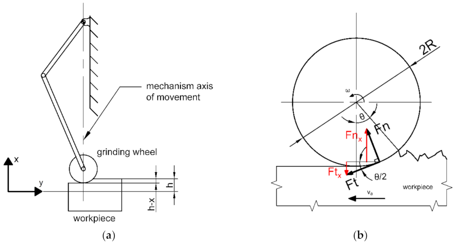
2. Deburring Forces
3. Proposed Mechanism
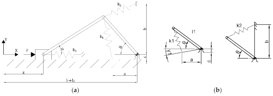
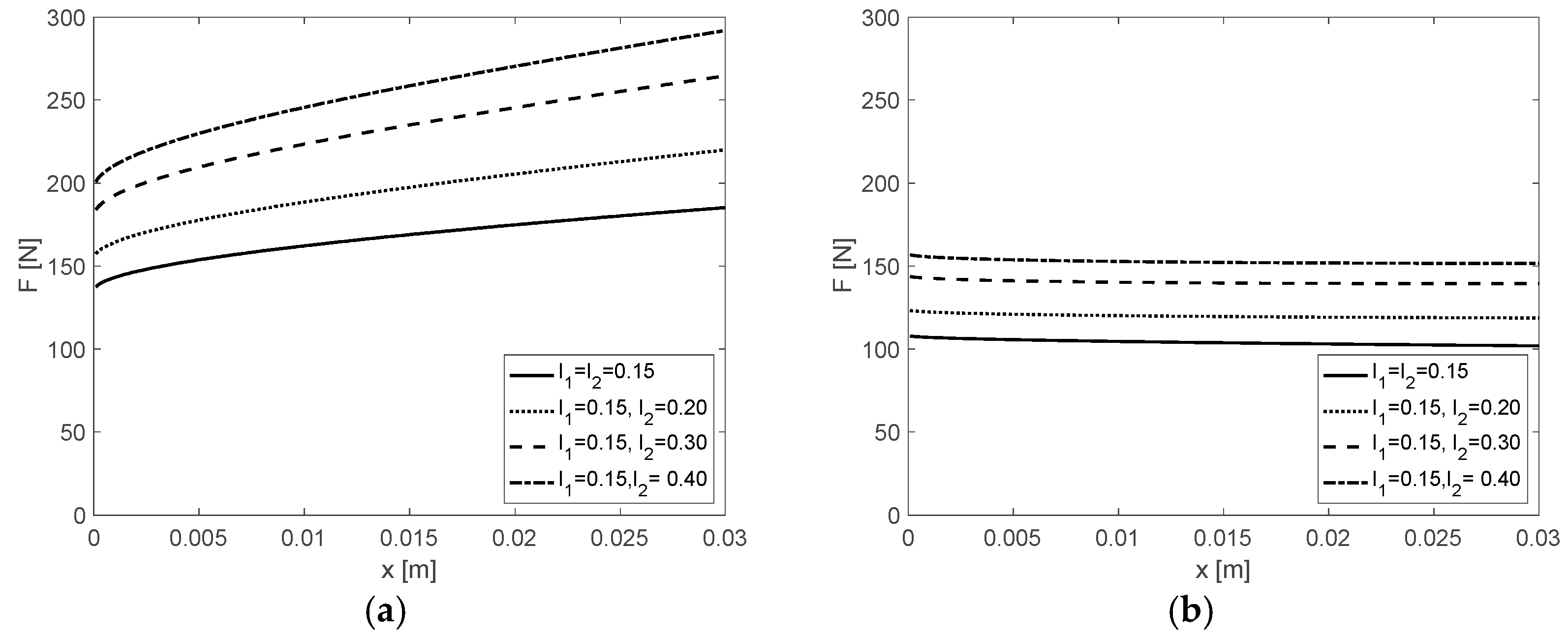
3.1. First Temptative Mechanism
3.2. Final Mechanism
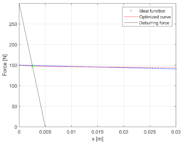
4. Design
5. Dynamic Analysis
5.1. Dynamic Model
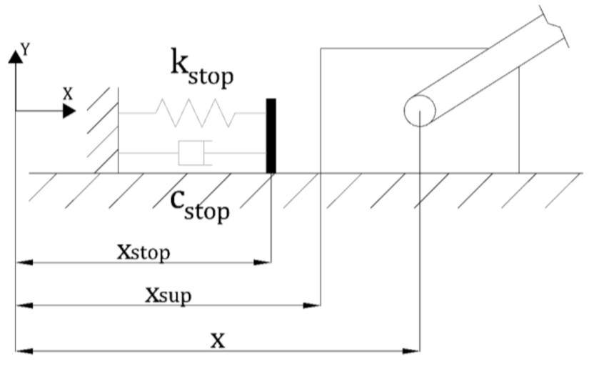
5.2. Mechanical Stop Model
- is the stiffness of the mechanical stop;
- is the coordinate of the surface of the slider that impacts the mechanical stop;
- () and are the coordinates of the limits of the mechanical stop;
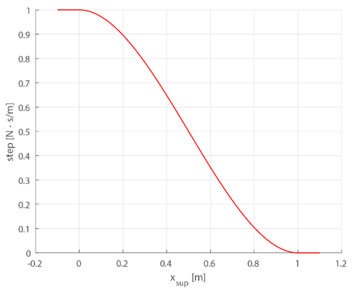
- is the exponent in (28), which is null in the case of the Kelvin-Voigt model;
- and are the limits of the function .
5.3. Simulation Results
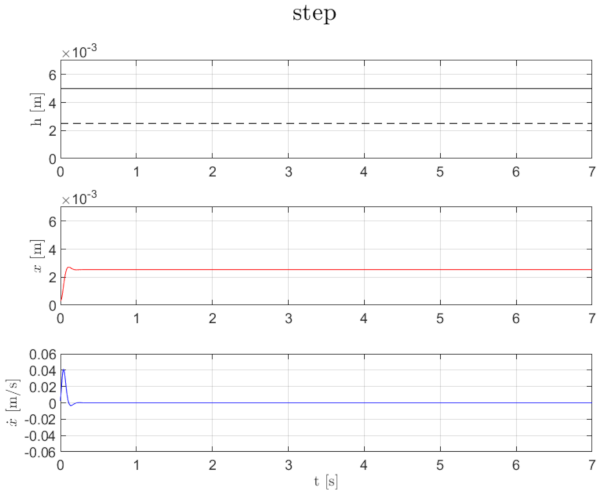
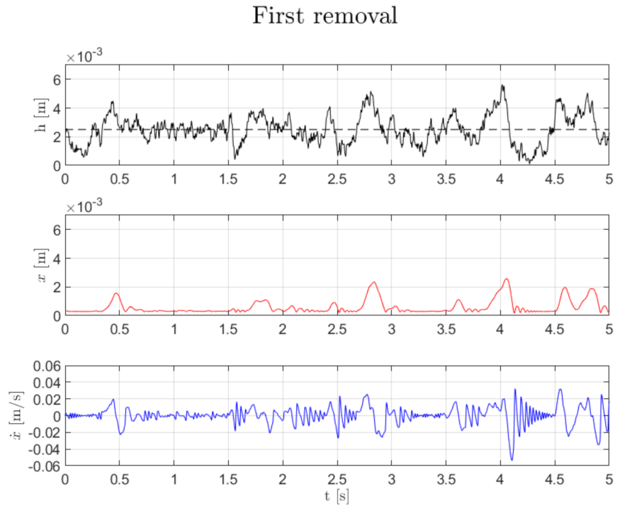
- If the projection of the cutting force along the sliding direction is less than the elastic force threshold of the mechanism, then the grinding wheel support should not move. This happens for small burr heights. With the considered setup (specified in Table 3), the elastic force threshold of the mechanism, which is equal to the elastic reaction force for , is N). This force threshold corresponds to a burr height of 2.5 mm with the considered setup.
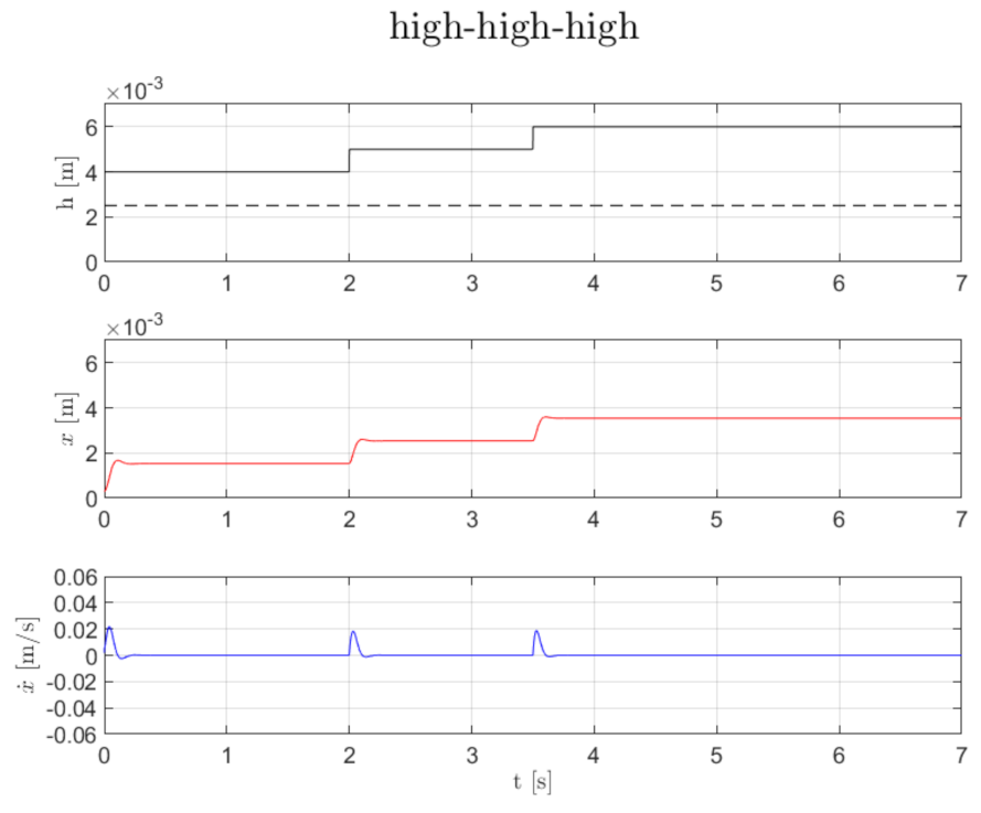
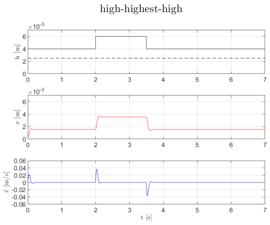
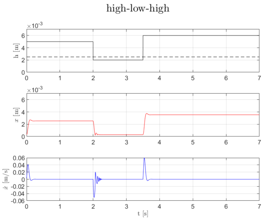
- If the projection of the cutting force along the sliding direction exceeds the elastic force threshold, the grinding wheel support should move backwards according to the compliance of the mechanism and the dynamics of (27); moreover, for a constant burr height, an equilibrium condition should be achieved (after a transient) between the cutting force projection and the elastic reaction force and, therefore, a cut profile with constant height should be obtained.
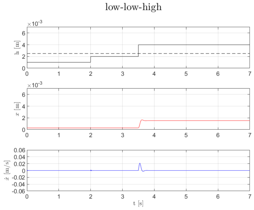
- If the burr height decreases, the compliant mechanism should move forward, and return towards the TDC. This condition is very important since it assures the stability of the system. Of course, even if the burr becomes very small, the mechanism can never reach the TDC due to the mechanical stop.
5.3.1. Test Case 1—1-Step Profile
5.3.2. Test Case 2—3-Steps Burr Profile “Low–Low–High”
5.3.3. Test Case 3—3-Steps Burr Profile “High–High–High”
5.3.4. Test Case 4—3-Steps Burr Profile “High–Highest–High”
5.3.5. Test Case 5—3-Steps Burr Profile “High–Low–High”
5.3.6. Test Case 6—Generic Burr Profile
6. Conclusions
Author Contributions
Funding
Institutional Review Board Statement
Informed Consent Statement
Data Availability Statement
Conflicts of Interest
References
- Onstein, I.F.; Semeniuta, O.; Bjerkeng, M. Deburring Using Robot Manipulators: A Review. In Proceedings of the 3rd International Symposium on Small-scale Intelligent Manufacturing Systems (SIMS), Gjøvik, Norway, 10–12 June 2020. [Google Scholar]
- Brunete, A.; Gambao, E.; Koskinen, J.; Heikkilä, T.; Kaldestad, K.B.; Tyapin, I.; Hovland, G.; Surdilovic, D.; Hernando, M.; Bottero, A.; et al. Hard material small-batch industrial machining robot. Robot. Comput. Integr. Manuf. 2018, 54, 185–199. [Google Scholar] [CrossRef]
- Pan, Z.; Zhang, H.; Zhu, Z.; Wang, J. Chatter analysis of robotic machining process. J. Mater. Process. Technol. 2006, 173, 301–309. [Google Scholar] [CrossRef]
- Cordes, M.; Hintze, W.; Altintas, Y. Chatter stability in robotic milling. Robot. Comput. Integr. Manuf. 2019, 55, 11–18. [Google Scholar] [CrossRef]
- Gillespie, L.K. Deburring and Edge Finishing Handbook; Society of Manufacturing Engineers: Southfiled, MI, USA, 1999. [Google Scholar]
- Li, W.; Wang, Y.; Fan, S.; Xu, J. Wear of diamond grinding wheels and material removal rate of silicon nitrides under different machining conditions. Mater. Lett. 2007, 61, 54–58. [Google Scholar] [CrossRef]
- Gillespie, L.K. Deburring precision miniature parts. Precis. Eng. 1979, 1, 189–198. [Google Scholar] [CrossRef]
- Babbar, A.; Jain, V.; Gupta, D. In vivo evaluation of machining forces, torque, and bone quality during skull bone grinding. Proceedings of the Institution of Mechanical Engineers, Part H. J. Eng. Med. 2020, 234, 626–638. [Google Scholar] [CrossRef] [PubMed]
- Babbar, A.; Jain, V.; Gupta, D.; Agrawal, D.; Prakash, C.; Singh, S.; Wu, L.Y.; Zheng, H.Y.; Królczyk, G.; Bogdan-Chudy, M. Experimental analysis of Wear and Multi-Shape Burr Loading during Neurosurgical Bone Grinding. J. Mater. Res. Technol. 2021, 12, 15–28. [Google Scholar] [CrossRef]
- Li, C.; Li, X.; Wu, Y.; Zhang, F.; Huang, H. Deformation mechanism and force modelling of the grinding of YAG single crystals. Int. J. Mach. Tools Manuf. 2019, 143, 23–37. [Google Scholar] [CrossRef]
- Tao, Y.; Zheng, J.; Lin, Y. A sliding mode control-based on a RBF neural network for deburring industry robotic systems. Int. J. Adv. Robot. Syst. 2016, 13, 8. [Google Scholar] [CrossRef] [Green Version]
- Qian, Y.; Yuan, J.; Bao, S.; Gao, L. Sensorless Hybrid Normal-Force Controller with Surface Prediction. In Proceedings of the IEEE International Conference on Robotics and Biomimetics (ROBIO), Yunnan, China, 6–8 December 2019. [Google Scholar]
- Pappachan, B.K.; Caesarendra, W.; Tjahjowidodo, T.; Wijaya, T. Frequency domain analysis of sensor data for event classification in real-time robot assisted deburring. Sensors 2017, 17, 1247. [Google Scholar] [CrossRef] [Green Version]
- Kakoi, H.; Yanagihara, K.; Akashi, K.; Tsuchiya, K. Development of Vertical Articulated Robot Deburring System by Using Sensor Feedback. In IOP Conference Series: Materials Science and Engineering; IOP: Bristol, UK, 2020. [Google Scholar]
- Hu, J.; Kabir, A.M.; Hartford, S.M.; Gupta, S.K.; Pagilla, P.R. Robotic deburring and chamfering of complex geometries in high-mix/low-volume production applications. In Proceedings of the IEEE 16th International Conference on Automation Science and Engineering (CASE), Virtual meeting, 20–21 August 2020. [Google Scholar]
- El Naser, Y.H.; Atali, G.; Karayel, D.; Özkan, S.S. Prototyping an Industrial Robot Arm for Deburring in Machining. Akad. Platf. Mühendislik Fen Bilimleri Derg. 2020, 8, 304–309. [Google Scholar]
- Guo, W.; Li, R.; Zhu, Y.; Yang, T.; Qin, R.; Hu, Z. A Robotic Deburring Methodology for Tool Path Planning and Process Parameter Control of a Five-Degree-of-Freedom Robot Manipulator. Appl. Sci. 2019, 9, 2033. [Google Scholar] [CrossRef] [Green Version]
- Lai, C.Y.; Chavez, D.E.V.; Ding, S. Transformable parallel-serial manipulator for robotic machining. Int. J. Adv. Manuf. Technol. 2018, 97, 2987–2996. [Google Scholar] [CrossRef]
- Vuong, N.-D.; Li, R.; Chew, C.-M.; Jafari, A.; Polden, J. A novel variable stiffness mechanism with linear spring characteristic for machining operations. Robotica 2017, 35, 1627. [Google Scholar] [CrossRef]
- Wang, W.; Fu, X.; Li, Y.; Yun, C. Design and implementation of a variable stiffness actuator based on flexible gear rack mechanism. Robotica 2018, 36, 448–462. [Google Scholar] [CrossRef]
- Barrett, E.; Reiling, M.; Barbieri, G.; Fumagalli, M.; Carloni, R. Mechatronic design of a variable stiffness robotic arm. In Proceedings of the IEEE/RSJ International Conference on Intelligent Robots and Systems (IROS), Vancouver, BC, Canada, 24–28 September 2017. [Google Scholar]
- Petit, F.; Daasch, A.; Albu-Schäffer, A. Backstepping Control of Variable Stiffness Robots. IEEE Trans. Control Syst. Technol. 2015, 23, 2195–2202. [Google Scholar] [CrossRef]
- Sciavicco, L.; Siciliano, B. Modelling and Control of Robot Manipulators; Springer Science & Business Media: Berlin/Heidelberg, Germany, 2012. [Google Scholar]
- Doria, A.; Cocuzza, S.; Comand, N.; Bottin, M.; Rossi, A. Analysis of the compliance properties of an industrial robot with the Mozzi axis approach. Robotics 2019, 8, 80. [Google Scholar] [CrossRef] [Green Version]
- Bottin, M.; Cocuzza, S.; Comand, N.; Doria, A. Modeling and identification of an industrial robot with a selective modal approach. Appl. Sci. 2020, 10, 4619. [Google Scholar] [CrossRef]
- Nemec, B.; Yasuda, K.; Ude, A. A Virtual Mechanism Approach for Exploiting Functional Redundancy in Finishing Operations. IEEE Trans. Autom. Sci. Eng. 2020. [Google Scholar] [CrossRef]
- Esquivel, E.; Carbone, G.; Ceccarelli, M.; Jáuregui, J.C. A Dynamic Compensation for Roll Hemming Process. IEEE Access 2018, 6, 18264–18275. [Google Scholar] [CrossRef]
- Görgülü, İ.; Carbone, G.; Dede, M.İ.C. Time efficient stiffness model computation for a parallel haptic mechanism via the virtual joint method. Mech. Mach. Theory 2020, 143, 103614. [Google Scholar] [CrossRef]
- Kalpakjian, S. Manufacturing Processes for Engineering Materials; Pearson Education India: Tamil Nadu, India, 1984. [Google Scholar]
- Malkin, S.; Guo, C. Grinding Technology: Theory and Application of Machining with Abrasives; Industrial Press Inc.: New York, NY, USA, 2008. [Google Scholar]
- Marinescu, I.D.; Hitchiner, M.P.; Uhlmann, E.; Rowe, W.B.; Inasaki, I. Handbook of Machining with Grinding Wheels, 2nd ed.; CRC Press: Boca Raton, FL, USA, 2016. [Google Scholar]
- Her, M.G.; Kazerooni, H. Automated robotic deburring of parts using compliance control. J. Dyn. Sys. Meas. Control. 1991, 113, 60–66. [Google Scholar] [CrossRef]
- Shinozuka, M.; Deodatis, G. Simulation of stochastic processes by spectral representation. Appl. Mech. Rev. 1991, 44, 191–204. [Google Scholar] [CrossRef]


| Parameter | Mechanism #1 | Mechanism #2 |
|---|---|---|
| 0.15 m | ||
| [0.15, 0.2, 0.3, 0.4] m | ||
| 0.05 m | 0.14 m | |
| 0.15 m | 0.03 m | |
| 0.05 m | ||
| 1500 N/m | ||
| 3000 N/m | 0 | |
| 200 N/m | 0 | |
| 1560 N/m | 47 N/m | ≈0 N/m | 0.14 m | 0.028 m |
| Parameter | Value |
|---|---|
| 1 * 10−3 m | |
| 15 * 10−3 m/s | |
| (steel) | 30 * 109 J/m3 |
| 100 rad/s | |
| 0.1 m | |
| 0.75 | |
| 2000 Ns/m | |
| 1560 N/m | |
| 47 N/m | |
| 0 N/m | |
| 0.14 m | |
| 0.028 m | |
| 0.05 m | |
| 0.15 m | |
| 0.3 m | |
| 30 kg | |
| 1.0 kg | |
| 0.5 kg | |
| N/m | |
| 3 * 10−4 m | |
| 0 m | |
| 0 Ns/m | |
| Ns/m |
Publisher’s Note: MDPI stays neutral with regard to jurisdictional claims in published maps and institutional affiliations. |
© 2021 by the authors. Licensee MDPI, Basel, Switzerland. This article is an open access article distributed under the terms and conditions of the Creative Commons Attribution (CC BY) license (http://creativecommons.org/licenses/by/4.0/).
Share and Cite
Bottin, M.; Cocuzza, S.; Massaro, M. Variable Stiffness Mechanism for the Reduction of Cutting Forces in Robotic Deburring. Appl. Sci. 2021, 11, 2883. https://doi.org/10.3390/app11062883
Bottin M, Cocuzza S, Massaro M. Variable Stiffness Mechanism for the Reduction of Cutting Forces in Robotic Deburring. Applied Sciences. 2021; 11(6):2883. https://doi.org/10.3390/app11062883
Chicago/Turabian StyleBottin, Matteo, Silvio Cocuzza, and Matteo Massaro. 2021. "Variable Stiffness Mechanism for the Reduction of Cutting Forces in Robotic Deburring" Applied Sciences 11, no. 6: 2883. https://doi.org/10.3390/app11062883