Initial Estimation of Kinematic Structure of a Robotic Manipulator as an Input for Its Synthesis

Abstract

Researchers often deal with the synthesis of the kinematic structure of a robotic manipulator to determine the optimal manipulator for a given task. This approach can lower the cost of the manipulator and allow it to achieve poses that might be unreachable by universal manipulators in an existing constrained environment. Numerical methods are broadly used to find the optimum design but they often require an estimated initial kinematic structure as input, especially if local-optimum-search algorithms are used. This paper presents four different algorithms for such an estimation using the standard Denavit–Hartenberg convention. Two of the algorithms are able to reach a given position and the other two can reach both position and orientation using Bézier splines approximation and vector algebra. The results are demonstrated with three chosen example poses and are evaluated by measuring manipulability and the total link length of the final kinematic structures.

1. Introduction

Nowadays, manufacturing industry, the most common type of robotic manipulator has six serial axes (degrees of freedom—DoFs) that are arranged in a so-called universal kinematic structure, e.g., the robots of ABB, KUKA, Fanuc, Yaskawa, and many others. In a very simplified way, the typical process for the deployment of a robot is to analyse the manufacturing process and workplace area first, followed by the choosing of a universal robotic manipulator and simulating the process. If the manipulator can reach the desired poses and fulfil the given task, further deployment can be considered.

However, using this universal kinematic structure is not always necessary, when a manipulator with fewer axes is suitable to perform the given task, or even possible, if the universal manipulator can face unavoidable collisions in an already existing environment. Additionally, they might not fulfil the desireed advanced operation conditions, such as manipulability [1] and kinematic reliability [2]. Therefore, researchers are focused on the topic of the synthesis of the kinematic structure of manipulators, which means finding such a kinematic structure that is optimal for a given task. This approach of deployment of highly customised manipulators may lead to benefits like lowered energy consumption, accelerated manufacturing process cycles, or deploying manipulators in highly dense-built workplaces. An example of such a general structure is presented by Brandstötter et al., who delivered the so-called curved manipulator (CuMa) [3] with possible modifications of its structure during the operational process [4]. This is achieved by changing the temperature in the links so they become flexible. A different approach to a deformable manipulator was taken by Xu et al. [5], where the links are composed of a few components and it is possible to change the orientation between them. Clark et al. [6] uses air pressure to change the kinematic structure of the presented malleable robot. The custom design of manipulators is desired not only in the manufacturing industry, but for example, in healthcare for helping with human upper limb rehabilitation [7] and shoulder joint rehabilitation [8].

There are two approaches to the synthesis of the kinematic structure of a manipulator. Analytically, it was solved by Hauenstein et al. [9] in the synthesis of three-revolute spacial chain for five poses. However, once a path becomes more complex and requires more degrees of freedom (more manipulator axes), the numerical approach is applied utilising optimisation algorithms. Among them, evolutionary robotics with genetic algorithms (GA) are probably the most common. Chocron et al. [10] used an adaptive multi-chromosome evolutionary algorithm to build a modular manipulator. Furthermore, GA can be used to build a manipulator from adaptive modules to perform a desired task [11]. Pastor et al. [12] compared straight, rounded, and curved mechanism links synthesised using GA. Valsamos et al. created so-called pseudo-joints (links which can be modified) and proposed a GA that tries to find the kinematic structure with the best manipulability [13]. It was later verified in an experiment with a real manipulator [14]. The synthesis of a parallel manipulator is addressed in [15]. As an example of non-industrial application, the work by Zeiaee et al. [16] deals with the optimisation of an eight-DoFs upper-limb exoskeleton.

In addition to GAs, the global optimum of an objective function can be searched with Simulated Annealing algorithm [17] or by a heuristic-guided tree search algorithm [18]. Another numerical method for finding the optimal manipulator for a given task is to search for a local minimum of an objective function. To solve this, a nonlinear programming (NLP) can be used, as it was implemented by Dogra et al. [19] for the design of a modular manipulator. In the paper, an optimal kinematic structure was proposed based on the minimisation of the joint torques. Another usage of NLP is trying to find an optimal design minimizing the path length in joint space [20].

The results of the already described papers [19,20] seem promising in their application of nonlinear programming to solve task-based custom manipulator design, however, there is one unanswered question in their work. In general, nonlinear programming traditionally requires that a starting point is given as part of the problem data, and comparative numerical testing is done using these traditional starting points [21]. In the case of robotic manipulators, if there is a given random path for a robotic manipulator, how should the starting point (initial values, initial estimation) of its kinematic structure look like?

The work [19] mentions a set of input values without any detailed explanation of how those values were determined. In [20], eight initial seeds are applied, but they are random values, which might be a cause of why no solution was found at all in some cases. In [17], they searched for a global optimum; however, the input values are also random, which may extend the time of solving the objective function. Even in a book by Ghafil et al. [22] which serves as an introduction to the optimisation of kinematic structures, the initial values for all described methods are obtained randomly without any detailed discussion. Therefore, a possible answer to the previously stated question will be addressed in this paper using multiple approaches.

In this paper, a geometric analysis to estimate kinematic structures and related calculations are proposed and discussed. The outcomes may avoid relying on randomness, which in the case of local-optimum-search algorithms may more frequently lead to convergence, making them reliable but still much faster than global-optimum-search methods. Moreover, the results can also be used in the previously mentioned algorithms using GAs, where they can serve as an optional first generation input, and in global-optimum-search algorithms, where they can reduce the time needed for the optimisation. In addition to that, the procedure may serve as an input for other custom manipulator design challenges such as collision avoidance [23].

A Denavit–Hartenberg notation [24] (standard DH parameters) was applied in the presented algorithms to obtain a general kinematic structure of a robot. The DH parameters were widely used, however, they also bring some disadvantages in the case of general structures. These are discussed later. Some algorithms behind the automatic placement of DH parameters have already been presented. In [25], a vector-algebra is applied to extract the parameters. Corke [26] creates a string of elementary translations and rotations from the user-defined base coordinate to the end-effector and factorises the string afterwards. An approach by Rajeevlochana et al. [27] is using line geometry to obtain the parameters. In addition to that, some researchers proposed their algorithms and they also identified (and verified) the DH parameters with an external sensor device in simulation [28] or experiments [29]. However, all of these algorithms were applied to already existing robots or similar devices. On the other hand, the algorithms presented in this paper are here to determine and “create” a non-existing manipulator (its kinematic structure) that can achieve a freely given pose.

2. Materials and Methods

When an algorithm is searching for a local minima of a function, the results may differ upon the choice of initial values. To find the optimal solution for two initial values with different outcomes, the cost function has to be compared afterwards. More accurate initial values can lead to fewer iterations that the algorithm needs, which can also save computing time. In this section, four algorithms of automatic assignment of DH parameters are presented, so they can serve as initial values for the synthesis of kinematic structure. The inputs are the position of the base of a robot, its tool-center point (TCP) pose, and the number of joints.

In this paper, we denote the transformation matrix between two frames as $\mathbf{J}$ with axis vectors and position coordinates as shown in Equation (1). The $\overrightarrow{n}$ (normal) is the X axis vector, the $\overrightarrow{o}$ (orientation) is Y axis vector, the $\overrightarrow{a}$ (approach) is Z axis vector, and the $\overrightarrow{t}$ (translation) is the position coordinate vector of a pose. $\mathbf{J}$ is a special Euclidean group of rigid body displacements in three dimensions (SE3) representing 3D rigid-body motion:

$$\mathbf{J}=\left[\begin{array}{cccc}& & & \\ \overrightarrow{n}& \overrightarrow{o}& \overrightarrow{a}& \overrightarrow{t}\\ & & & \\ 0& 0& 0& 1\end{array}\right]$$

(1)

We also use unit vectors of the X, Y, and Z axes. They are denoted as $\overrightarrow{i}$, $\overrightarrow{j}$, and $\overrightarrow{k}$:

$$\overrightarrow{i}=\left[\begin{array}{c}1\\ 0\\ 0\end{array}\right];\overrightarrow{j}=\left[\begin{array}{c}0\\ 1\\ 0\end{array}\right];\overrightarrow{k}=\left[\begin{array}{c}0\\ 0\\ 1\end{array}\right]$$

(2)

For visualisation and work with SE3 groups, we used the MATLAB^®, and Robotics Toolbox that was made by P. Corke. It is described in his book [30] and accessible as open source Github repository [31].

DH parameters are the most suitable and easily applicable technique for kinematic structures that have parallel or orthogonal axes. The typical procedure is that one has a robot and places the coordinate frames following the convention [24]. However, what to do when there is a given pose that is needed to be reached while no robot is chosen yet? This is the problem for the synthesis of kinematic structure. There is one important issue related to DH parameters. Between two general poses (right-hand rule following coordinate frames), it is uncertain if the transformation matrix ${\mathbf{J}}_{i-1,i}$ from $(i-1)$th pose to ith pose can be achieved following the typical procedure as the multiplication of a rotation matrix of ${\theta }_i$ around the $z_{i-1}$ axis, the translation matrix of $d_i$ along the $z_{i-1}$ axis, the translation matrix of $a_i$ along hte $x_i$ axis, and the rotation matrix of ${\alpha }_i$ around the $x_i$ axis, as shown in the following equations:

$$\mathrm{R}\mathrm{o}\mathrm{t}(z_{i-1},{\theta }_i)=\left[\begin{array}{cccc}\mathrm{c}\mathrm{o}\mathrm{s}\theta & -\mathrm{s}\mathrm{i}\mathrm{n}\theta & 0& 0\\ \mathrm{s}\mathrm{i}\mathrm{n}\theta & \mathrm{c}\mathrm{o}\mathrm{s}\theta & 0& 0\\ 0& 0& 1& 0\\ 0& 0& 0& 1\end{array}\right]$$

(3)

$$\mathrm{T}\mathrm{r}\mathrm{a}\mathrm{n}\mathrm{s}(z_{i-1},d_i)=\left[\begin{array}{cccc}1& 0& 0& 0\\ 0& 1& 0& 0\\ 0& 0& 1& d_i\\ 0& 0& 0& 1\end{array}\right]$$

(4)

$$\mathrm{T}\mathrm{r}\mathrm{a}\mathrm{n}\mathrm{s}(x_i,a_i)=\left[\begin{array}{cccc}1& 0& 0& a_i\\ 0& 1& 0& 0\\ 0& 0& 1& 0\\ 0& 0& 0& 1\end{array}\right]$$

(5)

$$\mathrm{R}\mathrm{o}\mathrm{t}(x_i,{\alpha }_i)=\left[\begin{array}{cccc}1& 0& 0& 0\\ 0& \mathrm{c}\mathrm{o}\mathrm{s}\alpha & -\mathrm{s}\mathrm{i}\mathrm{n}\alpha & 0\\ 0& \mathrm{s}\mathrm{i}\mathrm{n}\alpha & \mathrm{c}\mathrm{o}\mathrm{s}\alpha & 0\\ 0& 0& 0& 1\end{array}\right]$$

(6)

$${\mathbf{J}}_{i-1,i}=\mathrm{R}\mathrm{o}\mathrm{t}(z_{i-1},{\theta }_i)\mathrm{T}\mathrm{r}\mathrm{a}\mathrm{n}\mathrm{s}(z_{i-1},d_i)\mathrm{T}\mathrm{r}\mathrm{a}\mathrm{n}\mathrm{s}(x_i,a_i)\mathrm{R}\mathrm{o}\mathrm{t}(x_i,\alpha )$$

(7)

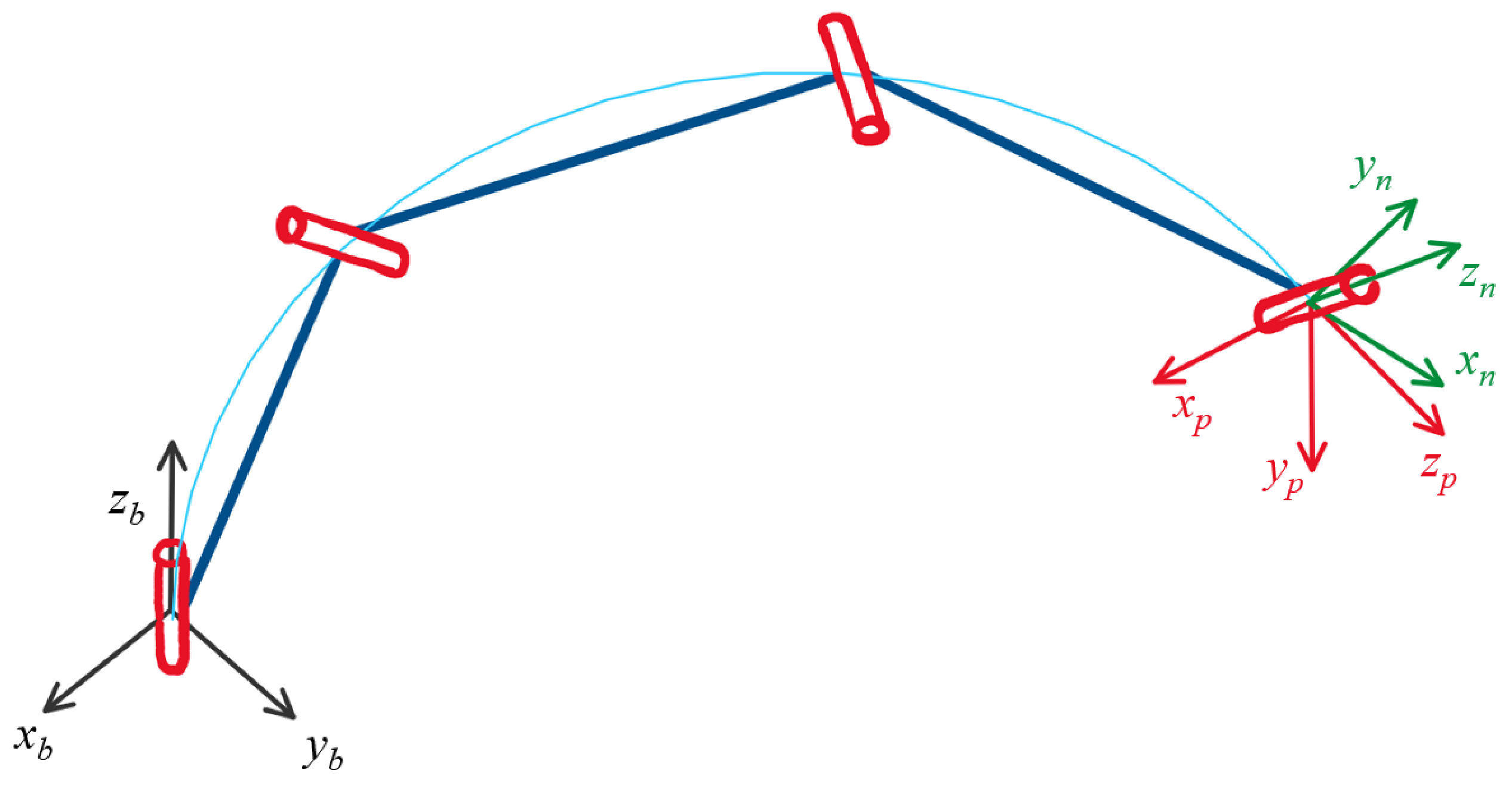
It is clear that rotation and translation around and along the y axis are missing to achieve all possible poses. In DH convention, it is mitigated by placing the joint coordinate frames in a specific way and applying Equation (7), as explained in [24]. However, if there are two general poses $(i-1)$th and ith which do not follow DH convention, it is possible to find a common perpendicular between their two $z_{i-1}$ and $z_i$ axes. Please see Figure 1. Rotation around $z_{i-1}$ to the direction of the perpendicular is ${\theta }_i$. $d_i$ is the distance from the $x_{i-1}$ axis to the intersection point P of the perpendicular and $z_{i-1}$ axis. The distance along the perpendicular is equal to the $a_i$ distance between these two frames. Finally, the rotation around the $x_i$ axis to the direction of $z_i$ is ${\alpha }_i$. If another displacement of $d_{i+1}$ is added and a rotation ${\theta }_{i+1}$ is applied, the previously unreachable (by four DH parameters) general pose ith becomes achievable by four DH parameters of $(i-1)$th joint and two DH parameters $d_{i+1}$ and ${\theta }_{i+1}$ of the ith joint. It can also represent an end-effector coordinate frame if the $(i-1)$th joint was the last joint. This approach is presented in detail in [27,29]. For the following calculations, we enhanced a script made by Brodsky [32] to find a common perpendicular and intersection points P and Q. This can be found in the Supplementary Material of this paper.

We used 3 poses to demonstrate the strong and weak points of the four presented algorithms to synthesise manipulators guiding their end-effector through the given position or pose, so everyone can choose the right solution for its implementation. They are also compared in Section 3 by manipulability and arm length. The first pose is a general one. The second pose is also general, but with a small offset between its Z axis and the Z axis of the base frame. The third pose has the parallel Z axis with the base Z axis. The poses are visualised in Figure 2:

$$Pose\left(1\right)=\left[\begin{array}{cccc}-0.50& -0.18& -0.84& -1.0\\ -0.06& 0.98& -0.17& 0.9\\ 0.86& -0.02& -0.50& 0.8\\ 0& 0& 0& 1\end{array}\right]$$

(8)

$$Pose\left(2\right)=\left[\begin{array}{cccc}0.81& -0.34& -0.46& -0.4\\ 0.48& -0.02& 0.87& 0.6\\ -0.30& -0.93& 0.14& 0.7\\ 0& 0& 0& 1\end{array}\right]$$

(9)

$$Pose\left(3\right)=\left[\begin{array}{cccc}0& 1& 0& 0.4\\ 1& 0& 0& 0.6\\ 0& 0& -1& 0.7\\ 0& 0& 0& 1\end{array}\right]$$

(10)

Two of the four presented algorithms utilised Bézier curves (splines) which are easy to implement between two given coordinate frames. For the presented calculations, only four control points are required to define a Bézier curve. We used a script by Bai [33] to calculate the curve. The control points $P_{1-4}$ were calculated using the following equations, where ${\overrightarrow{t}}_b$ is the base point coordinate, ${\overrightarrow{t}}_p$ is the pose point coordinate, ${\overrightarrow{a}}_b$ is the rotational vector of the Z axis of the base, ${\overrightarrow{a}}_p$ is the rotational vector of the Z axis of the pose, and p is the parameter related to the Euclidean distance between the base and the pose. The Bézier splines are visualised in Figure 3 for the chosen poses.

$$P_1={\overrightarrow{t}}_b$$

(11)

$$P_2={\overrightarrow{t}}_b+p{\overrightarrow{a}}_b$$

(12)

$$P_3={\overrightarrow{t}}_p-p{\overrightarrow{a}}_p$$

(13)

$$P_4={\overrightarrow{t}}_p$$

(14)

$$p=\frac{\left|\right|{\overrightarrow{t}}_p-{\overrightarrow{t}}_b\left|\right|}{2}$$

(15)

The generated kinematic structures that have served as examples in this paper have 4 joints; however, the presented algorithms are general and can provide a solution from 3 to an unlimited number of joints. In the following subsections, all 4 procedures are presented. The types A and B only deal with the position (translational part) of a given pose, so they do not fulfil the given orientation. However, this might be enough in some cases. The other two types C and D are able to achieve a pose including orientation using the common perpendicular approach, but in some specific poses it generates structures with joints in collision. The A and C types are obtained using vector algebra only, and the B and D types use Bézier’s curve approximation.

Three variables are input for all presented algorithms. It is the transformation of the robot base, the transformation of the TCP pose, both with respect to the world coordinate frame, and the desired number of joints. In our case, the base is an identity matrix. We used 3 transformations of the poses presented before, and the number of joints is four, as already said.

2.1. Type A—The Nearest Distance to Achieve a Position

This simple structure is obtained by finding the distance between the poses projected into the XY base plane. Only a positional vector of a pose is reached while the orientation is not taken into account. The implementation of such a structure is easy and straightforward. The idea is presented in Figure 4:

The first step is to find the length of $a_{0..n}$—the distance between joints in the X axis direction. The length is the projection of ${\overrightarrow{t}}_p$, the pose position vector, in the XY plane of the base, so only the X and Y coordinates are applied in Equation (16). n is the number of joints:

$$a_{1..n}=\frac{\sqrt{{({\overrightarrow{t}}_{p,x}-{\overrightarrow{t}}_{b,x})}^2+{({\overrightarrow{t}}_{p,y}-{\overrightarrow{t}}_{b,y})}^2}}{n}$$

(16)

Then, find the length of $d_1$—the offset of the joint along the Z axis. Only the Z axis coordinates of the two position vectors are applied:

$$d_1={\overrightarrow{t}}_{p,z}-{\overrightarrow{t}}_{b,z}$$

(17)

The ${\theta }_{1..n}$ are joint variables, and their offset is set to 0 degrees. The other parameters, $d_{2..n}$ and ${\alpha }_{1..n}$ can be set either to zero or they can be freely defined as ±values, for example. We chose ${\alpha }_1=\pi /4$, ${\alpha }_2=-\pi /4$, etc. One must be careful in the case of an even/odd number of joints—the sum of such tweaks needs to be equal to zero.

2.2. Type B—Joints on Bézier Curve to Achieve a Position

This method places joints between the base and the pose on a Bézier curve. To be able to obtain DH parameters, the proposed algorithm is orienting the $(i-1)$th joint (its rotational matrix) in a way that the ith joint lies in the XZ plane of the previous joint. The schematic is shown in Figure 5:

Using Equations (11)–(15), the Bézier spline is approximated between a given base and a pose. The number of approximated points is equal to the number of joints n. $Q_{1..n}$ is the set of these points–coordinates of each point with respect to the base frame.

Let us define a set ${\mathbf{J}}_{1..n}$ of SE3 objects representing the translation and orientation of the joints in the manipulator’s default position. As a first step, all ${\mathbf{J}}_{1..n}$ are set to be equal to the given base (in our case, an identity matrix). We also define an SE3 object ${\mathbf{J}}_{n+1}$ representing the given end-effector pose. Now, for joints ${\mathbf{J}}_{2..n}$, the following procedure is done.

The ith joint is equal to the previous $(i-1)$th joint:

$${\mathbf{J}}_i={\mathbf{J}}_{i-1}$$

(18)

The frame ${\mathbf{J}}_i$ is translated on the Bézier curve changing its translation vector ${\overrightarrow{t}}_i$:

$${\overrightarrow{t}}_i=Q_i$$

(19)

The position vector ${\overrightarrow{t}}_i$ of ${\mathbf{J}}_i$ is expressed in the coordinate frame of the previous ${\mathbf{J}}_{i-1}$ using its inverse matrix:

$${\overrightarrow{t^{\prime }}}_i={\mathbf{J}}_{i-1}^{-1}{\overrightarrow{t}}_i$$

(20)

A projection of the ${\overrightarrow{t}}_i$ vector in the XY plane of the ${\mathbf{J}}_{i-1}$ frame is determined:

$${\overrightarrow{t^{″}}}_i={\overrightarrow{t^{\prime }}}_i-\left[\begin{array}{c}0\\ 0\\ {\overrightarrow{t^{\prime }}}_{i,z}\end{array}\right]$$

(21)

The angle ${\theta }_i$ (DH parameter) between the unit vector $\overrightarrow{i}$ of the ${\mathbf{J}}_{i-1}$ frame and the projection of the ${\overrightarrow{t}}_i$ vector is calculated as

$${\theta }_i={tan}^{-1}\left(\frac{\left|\right|\overrightarrow{i}\times {\overrightarrow{t^{″}}}_i\left|\right|}{\overrightarrow{i}·{\overrightarrow{t^{″}}}_i}\right)$$

(22)

While using a right-handed coordinate frame, it is necessary to check if an angle is rotating around an axis in the positive (counter clockwise) or negative (clockwise) direction. To determine this, we used the projection property of the dot product between the two vectors. In this case, if the dot product of the X${}_i$ axis is in the negative direction of the Y${}_{i-1}$ axis, the angle ${\theta }_i$ has to be multiplied by $-1$:

$${\theta }_i=\left\{\begin{array}{cc}-{\theta }_i,\hfill & \mathbf{if}\overrightarrow{j}·{\overrightarrow{t^{″}}}_i<0\hfill \\ {\theta }_i,\hfill & \mathbf{otherwise}\hfill \end{array}\right.$$

(23)

Now, ${\mathbf{J}}_i$ can be updated using the matrix multiplication:

$${\mathbf{J}}_i={\mathbf{J}}_i\mathrm{R}\mathrm{o}\mathrm{t}(z_{i-1},{\theta }_i)$$

(24)

Thanks to the known translations, ${}_i$ and $a_i$, between the frames (from the Bézier curve approximation), and the calculated ${\theta }_i$, only the angle ${\alpha }_i$ is missing among the DH parameters. The steps to determine it are similar as in the case of $\theta$. Following the DH convention, the ith and $(i+1)$th frames are involved.

The position vector of ${\mathbf{J}}_{i+1}$ on the Bézier curve is given:

$${\overrightarrow{t}}_{i+1}=Q_{i+1}$$

(25)

Position vector ${\overrightarrow{t}}_{i+1}$ of ${\mathbf{J}}_{i+1}$ is expressed in the coordinate frame of the currently determining frame ${\mathbf{J}}_i$ using its inverse matrix:

$${\overrightarrow{t^{\prime }}}_{i+1}={\mathbf{J}}_i^{-1}{\overrightarrow{t}}_{i+1}$$

(26)

A projection of the ${\overrightarrow{t}}_{i+1}$ vector in the YZ plane of the ${\mathbf{J}}_i$ frame is calculated:

$${\overrightarrow{t^{″}}}_{i+1}={\overrightarrow{t^{\prime }}}_{i+1}-\left[\begin{array}{c}{\overrightarrow{t^{\prime }}}_{i+1,x}\\ 0\\ 0\end{array}\right]$$

(27)

The angle ${\alpha }_i$ is between the unit vector $\overrightarrow{k}$ of the ${\mathbf{J}}_i$ frame and the projection of the ${\overrightarrow{t}}_{i+1}$ vector, calculated as the inverse tangent fraction of the cross and dot products of those two vectors:

$${\alpha }_i={\tan }^{-1}\left(\frac{\left|\right|\overrightarrow{k}\times {\overrightarrow{t^{″}}}_{i+1}\left|\right|}{\overrightarrow{k}·{\overrightarrow{t^{″}}}_{i+1}}\right)$$

(28)

Using a right-hand rule for coordinate frames, if the dot product of the Z${}_i$ axis is in the negative direction of the Y${}_{i+1}$ axis, the angle ${\theta }_i$ has to be multiplied by $-1$. Y${}_{i+1}$ is calculated as a cross product of ${\overrightarrow{t^{″}}}_{i+1}$ and $\overrightarrow{i}$ vectors:

$${\alpha }_i=\left\{\begin{array}{cc}-{\alpha }_i,\hfill & \mathbf{if}({\overrightarrow{t^{″}}}_{i+1}\times \overrightarrow{i})·\overrightarrow{k}<0\hfill \\ {\alpha }_i,\hfill & \mathbf{otherwise}\hfill \end{array}\right.$$

(29)

Now, the final form of ${\mathbf{J}}_i$ that fulfils the DH convention between $(i-1)$th and ith can be obtained:

$${\mathbf{J}}_i={\mathbf{J}}_i\mathrm{R}\mathrm{o}\mathrm{t}(x_i,{\alpha }_i)$$

(30)

This procedure works smoothly for all joints. However, it will probably not be possible to obtain such DH parameters between the last joint ${\mathbf{J}}_n$ and the given pose ${\mathbf{J}}_{n+1}$ to reach the pose with the right orientation. Therefore, this algorithm is extended as the type D estimation in Section 2.4.

2.3. Type C—Achieving a Pose with Common Perpendicular

This algorithm finds a common perpendicular between the Z axis of the base and the Z axis of the pose. The joints are placed on this perpendicular line, and the last joint is oriented in the direction of the Z axis. Both the position and orientation can be achieved using this approach, as Figure 6 shows.

At first, a common perpendicular and intersection points P and Q are determined between the Z${}_b$ and Z${}_p$ axes using the script made by Brodsky [32]. However, his algorithm was not providing good results if the 2 lines were parallel, so we enhanced it and added some functionality to mitigate this issue.

The next step is to calculate the angle ${\alpha }_{sum}$ between those two axes:

$${\alpha }_{sum}={\tan }^{-1}\left(\frac{\left|\right|\overrightarrow{a_b}\times \overrightarrow{a_p}\left|\right|}{\overrightarrow{a_b}·\overrightarrow{a_p}}\right)$$

(31)

Again, when using a right-handed coordinate system, it is necessary to determine whether the angle is positive or negative. We check the pose Z${}_{i+1}$ axis as a projection in the base Y${}_i$ axis:

$${\alpha }_{sum}=\left\{\begin{array}{cc}-{\alpha }_{sum},\hfill & \mathbf{if}\overrightarrow{o_b}·\overrightarrow{a_p}<0\hfill \\ {\alpha }_{sum},\hfill & \mathbf{otherwise}\hfill \end{array}\right.$$

(32)

${\alpha }_{1..n}$ is the angle between the Z axes of particular joints:

$${\alpha }_{1..n-1}=\frac{{\alpha }_{sum}}{n-1}$$

(33)

$${\alpha }_n=0$$

(34)

Now, we can calculate the rest of the DH parameters. $a_{1..n}$ is the distance between the joints. l is the length of a common perpendicular, and n is the number of joints:

$$a_{1..n-1}=\frac{l}{n-1}$$

(35)

$$a_n=0$$

(36)

$d_0$ is the distance from the base coordinate frame to the P-intersection point of the $\overrightarrow{a_b}$ and common perpendicular. $d_n$ is the distance from the Q, the intersection point of the $\overrightarrow{a_p}$ and a common perpendicular, to the pose coordinate frame. $d_n$ is also the translation of the end-effector from the last joint:

$$d_0=(P-\overrightarrow{t_b})·\overrightarrow{a_b}$$

(37)

$$d_{1..n-1}=0$$

(38)

$$d_n=(\overrightarrow{t_p}-Q)·\overrightarrow{a_p}$$

(39)

2.4. Type D—Joints on Bézier Curve while the Last Lies on Common Perpendicular to Achieve a Pose

This method extends type B estimation by adding a common perpendicular approach, used in type C, between the two last joints. This assures reaching the pose including orientation, as shown in Figure 7. The beginning steps are the same as in type C, but only from ${\mathbf{J}}_1$ to ${\mathbf{J}}_{n-1}$. The transformation of the last joint is determined using the following procedure.

Again, a common perpendicular and the intersection points P and Q are found between the joint ${\mathbf{J}}_{n-1}$ and the TCP pose ${\mathbf{J}}_{n+1}$ using the already presented ways. ${\mathbf{J}}_n$ is set equal to ${\mathbf{J}}_{n-1}$:

$${\mathbf{J}}_n={\mathbf{J}}_{n-1}$$

(40)

Angle ${\theta }_n$ between X${}_{n-1}$ and X${}_n$ axes is obtained:

$${\theta }_n={\mathrm{t}\mathrm{a}\mathrm{n}}^{-1}\left(\frac{\left|\right|{\overrightarrow{n}}_{n-1}\times \overrightarrow{PQ}\left|\right|}{{\overrightarrow{n}}_{n-1}·\overrightarrow{PQ}}\right)$$

(41)

Right-hand rule check is performed:

$${\theta }_n=\left\{\begin{array}{cc}-{\theta }_n,\hfill & \mathbf{if}{\overrightarrow{o}}_{n-1}·\overrightarrow{PQ}<0\hfill \\ {\theta }_n,\hfill & \mathbf{otherwise}\hfill \end{array}\right.$$

(42)

${\mathbf{J}}_n$ is rotated around Z${}_{n-1}$ axis afterwards:

$${\mathbf{J}}_n={\mathbf{J}}_n\mathrm{R}\mathrm{o}\mathrm{t}(z_{n-1},{\theta }_n)$$

(43)

Translation of the ${\mathbf{J}}_n$ along the Z${}_n$ and X${}_n$ is obtained by changing its translational vector $\overrightarrow{t_n}$, and it is equal to the coordinates of point Q:

$${\overrightarrow{t}}_n=Q$$

(44)

Angle ${\alpha }_n$ between Z${}_n$ and Z${}_{n+1}$ axes is calculated:

$${\alpha }_n={\mathrm{t}\mathrm{a}\mathrm{n}}^{-1}\left(\frac{\left|\right|\overrightarrow{a_n}\times {\overrightarrow{a}}_{n+1}\left|\right|}{\overrightarrow{a_n}·{\overrightarrow{a}}_{n+1}}\right)$$

(45)

Right-hand rule check, if the dot product of Z${}_{i+1}$ axis is in the positive direction of the Y${}_i$ axis, the angle ${\alpha }_n$ has to be multiplied by $-1$:

$${\alpha }_n=\left\{\begin{array}{cc}-{\alpha }_n,\hfill & \mathbf{if}\overrightarrow{o_n}·{\overrightarrow{a}}_{n+1}>0\hfill \\ {\alpha }_n,\hfill & \mathbf{otherwise}\hfill \end{array}\right.$$

(46)

The final transformation matrix of the last joint ${\mathbf{J}}_n$ is obtained:

$${\mathbf{J}}_n={\mathbf{J}}_n\mathrm{R}\mathrm{o}\mathrm{t}(x_n,{\alpha }_n)$$

(47)

From this point, when all frames ${\mathbf{J}}_{1..n}$ representing the joints are known, it is possible to derive the DH parameters between them.

3. Results

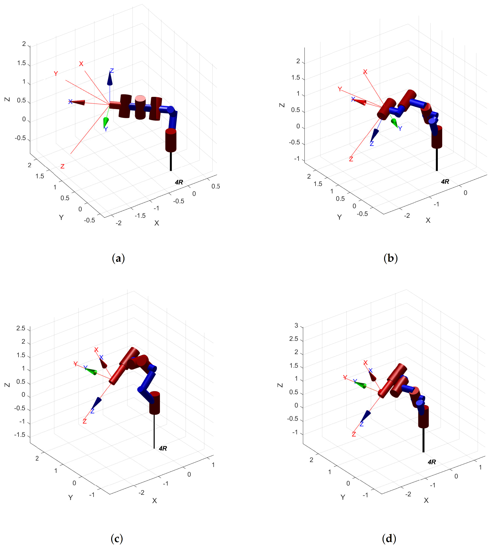
This section presents the kinematic structures generated by the presented algorithms for the three poses defined earlier (Figure 2). The results are discussed and later compared by manipulability measure and manipulator length. A table with calculated DH parameters is also included. The visualisation of the final kinematic structures is shown in Figure 8, Figure 9 and Figure 10.

The types of estimation A and B are not able to reach a pose in terms of orientation in general; however, in some cases (as shown in Figure 10b) the real solution was found for the type B. In addition, if compared with a similar D result (Figure 10d) for $Pose\left(3\right)$, solution B provides shorter links. Furthermore, the A and B types are generated in a way where no collision of joints should occur.

The type C may perform very well if the Z axes of the base and pose are parallel, as shown in Figure 10c; on the other hand, if the axes are very close to each other (the perpendicular distance is short), the joints are in collision, as shown in Figure 9c.

Placing joints on an approximated spline provides the most general result of the provided algorithms, as shown in Figure 8d and Figure 9d, but it is struggling with parallel axes—see Figure 10d. This could be mitigated by tuning the Bézier curve driven point related to the pose and placing the joints not in a plane that is defined by the two parallel Z axes.

3.1. Resulting DH Parameters

For a better evaluation, we include

Table 1. The DH parameters of manipulators for $Pose\left(1\right)$.

Joint	${\mathit{d}}_{\mathit{i}}$ (m)	${\mathit{a}}_{\mathit{i}}$ (m)	${\mathit{\alpha }}_{\mathit{i}}$ (rad)	Joint	${\mathit{d}}_{\mathit{i}}$ (m)	${\mathit{a}}_{\mathit{i}}$ (m)	${\mathit{\alpha }}_{\mathit{i}}$ (rad)
1	0.8	0.34	0.79	1	0.64	0.29	−0.39
2	0	0.34	−0.79	2	0.32	0.56	−1.48
3	0	0.34	0.79	3	0.46	0.38	0
4	0	0.34	−0.79	4	0	0	−0.28
a Type A estimation				b Type B estimation
Joint	${\mathit{d}}_{\mathit{i}}$(m)	${\mathit{a}}_{\mathit{i}}$(m)	${\mathit{\alpha }}_{\mathit{i}}$(rad)	Joint	${\mathit{d}}_{\mathit{i}}$(m)	${\mathit{a}}_{\mathit{i}}$(m)	${\mathit{\alpha }}_{\mathit{i}}$(rad)
1	1.27	0.36	−0.7	1	0.64	0.29	−0.40
2	0	0.36	−0.7	2	0.32	0.55	−1.48
3	0	0.36	−0.7	3	−0.33	0.30	−0.29
4	0.93	0	0	4	0.83	0	0
c Type C estimation				d Type D estimation

with the generated DH parameters for $Pose\left(1\right)$. The angles $\theta$ are considered as variables with zero offset.

3.2. Manipulator Length Comparison

In general, longer links of a manipulator demand more powerful motors because of higher torques. In Figure 11, there is a bar plot comparing the lengths of the resulting manipulators. The length was determined using Equation (48), where $a_i$ and $d_i$ are DH parameters of $i_{th}$ link. n is the number of joints:

$$L=\sum _{i=1}^n\sqrt{a_i^2+d_i^2}$$

(48)

3.3. Manipulability Comparison

To compare the results, we decided to evaluate the manipulability of the calculated kinematic structures. This scalar measure was obtained using the Yoshikawa algorithm [1], which describes how spherical the end-effector velocity ellipsoid is. It differs between 0 and 1, where the value 1 shows the best manipulability in all axes. If the value is close to 0, the mechanism might be dealing with singularities.

The results are shown for both translational and rotational motions in Figure 12 as a logarithmic graph, because the measure differs significantly between particular kinematic structures. It should be kept in mind that the presented manipulators have less than six DoFs, which is one of the reasons why the manipulability measure by Yoshikawa evaluates them with low numbers.

As expected, the type A kinematic structure has to deal with singularities and the manipulability tends to be the lowest for the given poses. Type B has almost the same translational manipulability as type D, but the last two joints are in a singular position, so the rotational manipulability drops in the case of type B kinematic structure. Type C performs better than types A and B. In the case of general poses $Pose(1,2)$, type D provides the highest manipulability measures. However, for $Pose\left(3\right)$ when Z axes are parallel, the manoeuvrability of the type D algorithm drops under the values of type C.

4. Discussion

The outcomes of this paper are aimed to be utilised in the synthesis of kinematic structures of robotic manipulators. Other applications are also possible, for example, in rapid kinematic analysis and simulation to evaluate kinematic options if only one position or pose on a trajectory is desired to be reached. However, only topics related to the synthesis problem are going to be discussed here.

This paper provided four algorithms to estimate the initial value of a kinematic structure for later implementation in optimisation algorithms. As mentioned previously, especially in algorithms searching the local minimum of an objective function, every initial guess can provide different results. Therefore, we decided to present the types (A and B) of estimation even though they do not fulfil the given pose in terms of orientation. The reason is that an optimisation algorithm may overcome this issue later and the solution could achieve the pose on a given trajectory with a better final value of the objective function than with the other presented types (C and D). This always depends on the type and properties of the trajectory. Therefore, we suggest implementing all four estimation types into an optimisation algorithm and compare the results afterwards.

If one would like to know which one of the four structures is the best, this question is not easy to answer. We chose three poses to demonstrate the advantages and disadvantages of particular algorithms and compared the final structures for these poses by manoeuvrability and length. The type D provides the most general structure that can reach any pose, but one must be careful in cases when some axes of the base and the pose are parallel, for example. We suggest to always visualise all initial structures for better evaluation.

The presented algorithms are based on the Denavit–Hartenberg convention, generating DH parameters. During this work, a question arose, of how suitable the DH convention is for general structures and especially for their synthesis for given trajectory. As mentioned previously, it is possible to find DH parameters between two coordinate frames using the common perpendicular approach, but it is required to “borrow” another two DH parameters from the next joint and to add them to the already existing four parameters. This is obvious since we need six parameters (three translations and three rotations) in general to describe the motion of a frame in Euclidean space. Therefore, using an optimisation algorithm to synthesise a manipulator that fulfils the DH convention may be limiting. The frames representing joints cannot freely rotate and translate wherever the algorithm tends to, but they have to follow the XZ planes in which the common perpendiculars between neighbouring joints lie. On top of that, the algorithm may not find the global or local minimum because of this limit at all. The reason is that traditionally DH parameters serve for the description of existing robots and once they are obtained, some local coordinates of the joints may be located outside of the rigid body along the Z axis, and although they are still closely tied to the particular joint and representing its kinematics, they are not representing the real (physical) position of the joint. On the other hand, in terms of synthesis when a rigid body does not exist yet, the location (transformation) of the coordinate frames of joints is the only known and crucial parameter and its variability should not be limited during the synthesis process anyhow.

The comparison of the synthesis of kinematic structure using DH convention and other standard approaches, such as screw theory [34] for instance, will be an interesting topic for future research. However, this matter has no impact on the work presented in this paper. The kinematic structures obtained using the four algorithms may be translated into any other standard description of the structure of a manipulator.

5. Conclusions

This paper presents four mathematical algorithms to find an initial estimation of a kinematic structure of a serial robotic manipulator. The input values are the number of joints, the position of the base of the manipulator, and the target pose of its TCP. The outputs are the standard DH parameters of a kinematic structure that can reach the given pose either by position or by position and orientation. The presented methods are applicable in the topic of synthesis of the kinematic structure of robotic manipulators, where they can serve as an initial guess of a structure.

The examples of three poses for all four algorithms are shown and compared using the manipulability measure and the arm length. However, it is not easy to determine which method out of these four is the best as it is always depending on the input, especially the TCP pose. The manipulability measure indicates that the D type algorithm, which can fully satisfy any given pose, provides the best manipulability in general, because it avoids placing joints on a single line and places them on a Bézier curve instead. In addition to that, the joints also tend to prevent collisions. On the other hand, if the given pose is representing a specific case, as a parallel axis or axes with a base frame axis or axes, one should be always watchful and comparison with the other presented algorithms is suggested. As expected, algorithm types A and B achieved the best results in the case of the arm length measure, when only a position is desired. However, in some cases, the C and D algorithms may fully achieve a pose with a manipulator with similarly long links.

Future steps are to implement this method in an optimisation algorithm and to observe if the convergence is faster or if the obtained result and the values of objective functions are better.

The algorithms were tested in MATLAB and the scripts are available as Supplementary Material for this paper or with eventual updates as an open source package on a public repository [35].