Article

Deep Transfer Learning for Machine Diagnosis: From Sound and Music Recognition to Bearing Fault Detection

by
Eugenio Brusa
,
Cristiana Delprete
and
Luigi Gianpio Di Maggio
*
Dipartimento di Ingegneria Meccanica e Aerospaziale (DIMEAS), Politecnico di Torino, Corso Duca Degli Abruzzi 24, 10129 Torino, Italy
*
Author to whom correspondence should be addressed.
Appl. Sci. 2021, 11(24), 11663; https://doi.org/10.3390/app112411663
Submission received: 9 November 2021 / Revised: 30 November 2021 / Accepted: 6 December 2021 / Published: 8 December 2021

Abstract

:
Today’s deep learning strategies require ever-increasing computational efforts and demand for very large amounts of labelled data. Providing such expensive resources for machine diagnosis is highly challenging. Transfer learning recently emerged as a valuable approach to address these issues. Thus, the knowledge learned by deep architectures in different scenarios can be reused for the purpose of machine diagnosis, minimizing data collecting efforts. Existing research provides evidence that networks pre-trained for image recognition can classify machine vibrations in the time-frequency domain by means of transfer learning. So far, however, there has been little discussion about the potentials included in networks pre-trained for sound recognition, which are inherently suited for time-frequency tasks. This work argues that deep architectures trained for music recognition and sound detection can perform machine diagnosis. The YAMNet convolutional network was designed to serve extremely efficient mobile applications for sound detection, and it was originally trained on millions of data extracted from YouTube clips. That framework is employed to detect bearing faults for the CWRU dataset. It is shown that transferring knowledge from sound and music recognition to bearing fault detection is successful. The maximum accuracy is achieved using a few hundred data for fine-tuning the fault diagnosis model.

1. Introduction

Although regular and scheduled maintenance strategies are still employed in many industrial contexts, the needs to rely on condition-based monitoring for machine health management have become increasingly pronounced due to several reasons. Industrial rotating systems are ever more complex, and wear and fatigue life estimators may not be accurate enough to properly schedule maintenance. Indeed, the useful life of some machine components is characterized by a marked statistical scatter, as in the case of rolling element bearings (REBs) [1]. On account of these aspects, early scheduled maintenance is likely to increase avoidable machine downtimes, whereas late scheduled maintenance leads to an unacceptable number of failures [2]. Moreover, the structural health of rotors and REBs affect each other in actual operating conditions, given the underlying coupling between their dynamic behavior. These issues hardly comply with the requirements of modern industry, which increasingly tends to embrace the advantages offered by condition-based monitoring in terms of cost savings and production targets attainment [3]. Machine fault diagnosis concerns the study of techniques aimed at detecting, isolating, and identifying machinery faults on the basis of monitoring data [4,5].
The last four decades have seen a growing interest towards this field within research and industry environments. In particular, signal processing methods have been extensively examined to uncover the links between vibration data [6,7,8,9,10,11,12,13] or acoustic emissions [14,15,16] and REB health state. Typically, these approaches stem from human reasoning, which infer expected particularities of data in light of the physical phenomena taking place in damaged REBs or, more generally, in defective industrial equipment. Nevertheless, monitoring data are simultaneously influenced by a variety of factors, such as noise and structural resonances. The superimposition of several sources of excitation further affect vibration responses. It may therefore occur that latent paths are hardly detectable in diagnostic features by the inferences of human intelligence, especially in real working conditions. For this reason, artificial intelligence (AI) found fertile ground for applications in vibration-based diagnostics and prognostics.
Research on intelligent fault diagnosis (IFD) [5] has consistently populated scientific literature starting from the beginning of this century. At first, machine learning approaches such as the support vector machine (SVM) [17,18,19,20] were mostly investigated. Later, deep learning and neural networks [21] revealed their capabilities in automatically identifying intricated as much as discriminative features in large image datasets [22] upon which machine learning algorithms were in trouble. IFD soon took advantage of these AI tools with the application of autoencoders [23,24], Convolutional neural networks (CNNs) [25,26,27] and Long Short-Term Memory networks (LSTMs) [28] for machinery diagnosis tasks. However, the encouraging results achieved by AI in fault diagnosis may present some limitations: lack of engineering interpretability and lack of a sufficient number of labelled data.
The interpretability of AI models is a current research topic in IFD [5,29] and its insights represent some future trends for research in the upcoming decade. Deep learning achieved unthinkable goals until about a few decades ago in manifold scenarios (e.g., computer vision, medicine, and speech recognition). This is also due to the availability of a sufficient number of labelled data for training deep architectures. However, a significant amount of data for faulty machines is barely available in practical engineering contexts [5]. In such cases, training processes are difficult to manage, since millions of network parameters are extremely prone to overfit small datasets. Thus, the ability to generalize the learned knowledge is intrinsically undermined. Noteworthy research efforts have brought to light benchmark datasets [30,31,32,33], on which several methodologies were tested. Compared with images datasets, it is experimentally challenging to extract millions of data which meaningfully portray probability distributions for machinery diagnosis.
Recently, transfer learning (TL) approaches began to address the problem of missing data [5,34]. The core idea of TL relates to the possibility of applying the knowledge learned in a source task to a target task. TL is inspired by the human brain which can intelligently use knowledge acquired in previous tasks to face new ones quicker or more efficiently [34]. TL strategies applied to machine fault diagnosis typically rely on networks pre-trained using images, to catch low-level features also in pictures drawn from vibration signal processing. This is partially occasioned by the fact that most of deep learning developed around images and CNNs. Consequently, several deep learning applications came across images for formalizing problems of various kinds. One of the largest datasets to train AI models for image recognition is ImageNet (https://www.image-net.org/, accessed on 29 October 2021) [35]. Currently, the dataset contains more than 14 million images, and over the past ten years, it has been extensively used to train deep learning architectures in extracting discriminative features of images for classifying them.
Applications of knowledge transfer for machine diagnosis using ImageNet are available in the literature. Shao et al. [36] successfully classified machine failures using neural networks pre-trained on ImageNet. Cao et al. [37] showed that a small set of training data is adequate to effectively perform a gear fault diagnosis using deep architectures trained with ImageNet. Instead, Zhang et al. [38] and Hasan and Kim [39] employed TL to diagnose machine failures, by transferring knowledge between different working conditions.
However, no previous studies have investigated knowledge transfer from sound recognition tasks to machine diagnosis. The present work is motivated by the idea that networks pre-trained on audios for sound event detection (SED) [40,41,42] may encapsulate the necessary knowledge to classify REB spectrograms. The main goal of SED is to identify instances of sound events in audio recordings [40,43]. Applications of machine listening are available for instance in the fields of traffic monitoring [44], smart rooms [45], autonomous vehicles [46] and healthcare monitoring [47]. Identifying music, instruments or music genres is among the capabilities of SED networks [48,49].
The search for bearings characteristic tones in vibration signals is conceptually similar to pitch identification in sound, speech and music recognition. Then, detecting occurrences of bearing failures through vibrations is not so different from identifying sound events in audio signals. It is therefore reasonable to assume that the knowledge required to label spectrograms originated from faulty bearings is partially enclosed in pre-trained SED networks, since some of these have specifically learned to extract dominant patterns in spectrograms.
May the knowledge gained in these tasks be transferred to characterize machine vibrations? Is this transfer strategy successful for a small dataset? These are the questions which moved this investigation. Obviously, vibration signals are not audio acquisitions, but they can be pre-processed in similar ways to deal with SED networks. Indeed, SED networks operate with feature spaces pursuant to the human perception of the sound. This study shows that this knowledge transfer efficiently works for a small dataset containing vibration signals.
The overall structure of this paper takes the form of six sections. The introduction presented the condition-based monitoring topic and projected AI advantages and issues in the field of machine diagnosis. An overview of CNNs and TL theoretical background is provided in the second section. The third section introduces YAMNet, an efficient CNN for sound detection. This deep architecture is employed in the fourth section for detecting bearing faults in a limited data scenario. Findings are discussed in the fifth section, and finally some concluding remarks are provided in the sixth section.

2. Theoretical Background

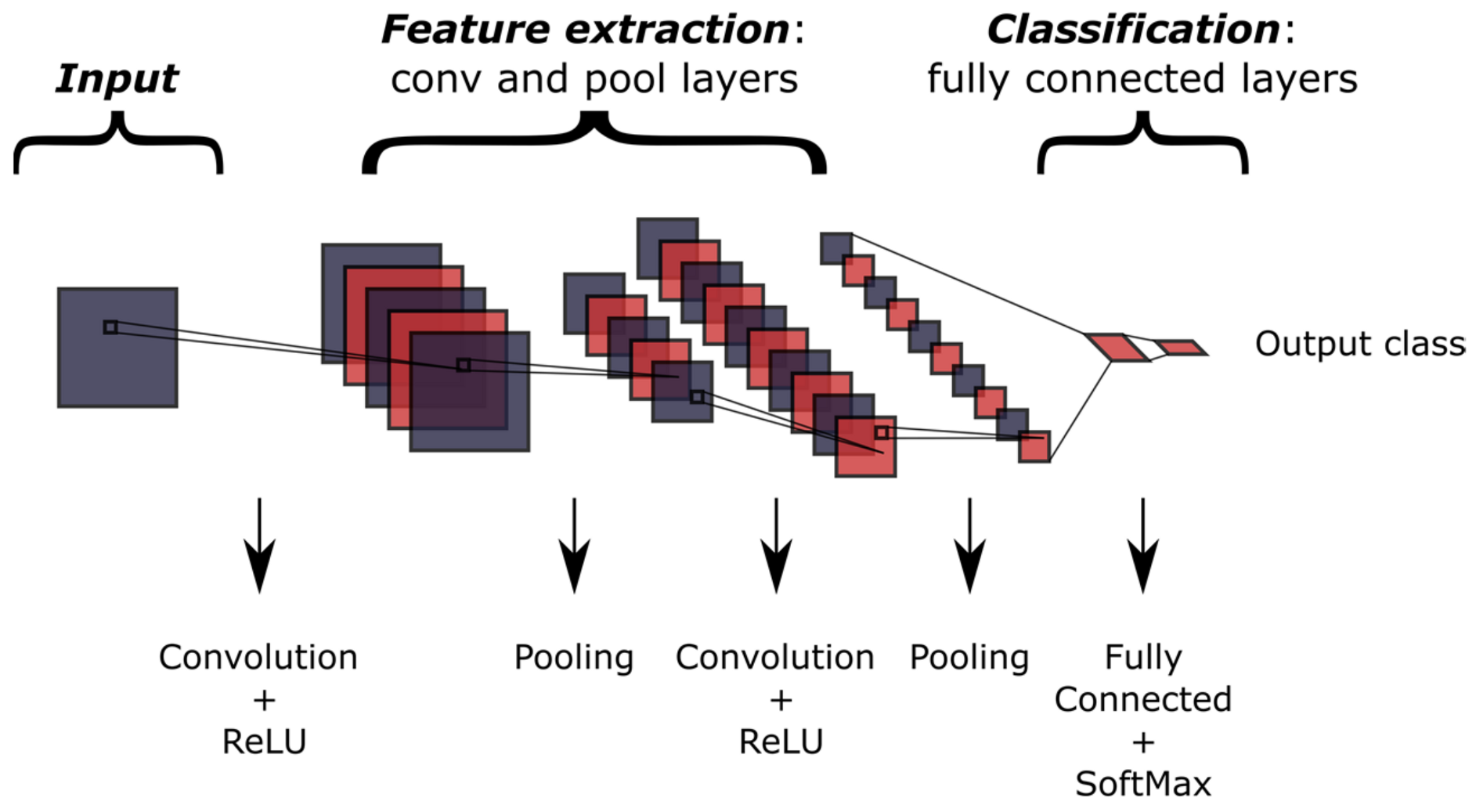
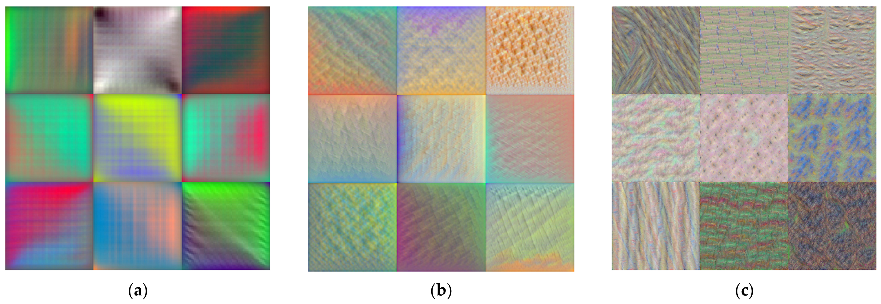
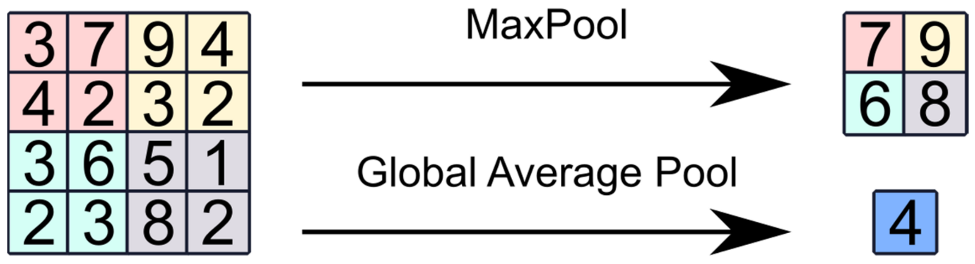
2.1. Convolutional Neural Networks (CNNs)

Convolutional neural networks (CNNs) consist of deep layered architectures, in which multidimensional algebra operations are carried out sequentially. These architectures match especially well with multidimensional data since the spatial information of the latter is preserved while being treated. For instance, the algebraic representation of RGB images needs two dimensions for populating pixel matrices, and a third dimension for RGB channels. The capabilities of CNNs were originally exploited for image classification tasks [22,50], but nowadays the potentials of these deep architectures are acknowledged in numerous fields concerning multidimensional data [25,26,27,42,51]. Generally, CNNs include three types of layers, corresponding to specific operations: convolution, pooling, and fully connected layers (Figure 1).
Convolutional layers convolve input tensors x l 1 of the layer l 1 by using filter kernels k l [5,51,52] as reported in Equation (1):
x l = σ x l 1 k l + b l
where is the convolution operator, b l the bias term of the layer l , and σ an activation function, which introduces nonlinear effects. Rectified Linear Unit (ReLU) is one of the most common activation functions for convolutional layers: R e L U x = max 0 , x . The output of the convolutional layer is the feature map x l . A training process essentially attempts at optimizing the elements of the kernel k l . Such an optimization produces output feature maps that emphasize the most significant attributes for categorizing input data. This aspect is factually the core idea underlying automated feature extraction in CNNs, which apprehend dominant patterns in training data. The feature extraction occurring in stacked convolutional layers is a hierarchical process: first convolutional layers typically learn general and low-level features, whereas deeper layers learn more complex, specific, and high-level features. Figure 2 shows an example of hierarchical feature learning for the well-known CNN AlexNet [22] trained on the ImageNet dataset. Such representations can be produced by passing a random noise image through the network for several iterations. Namely, the input noise is gradually modified by updating the network gradient in order to maximize the activation of a chosen layer. Then, the convolutional structure outputs images that mostly activate the channels of the specific layer. These maps highlight the features learned by the network in such a layer.
Pooling layers usually follow convolutional layers in CNNs architectures (Figure 1). The output of pooling layers is a low-resolution feature map, which is obtained through downsampling the input map. Pooling operations reduce the number of network parameters in order to mitigate data overfitting. Furthermore, the low-dimensional outputs of pooling layers extract local features, while preserving the multidimensionality of data. An example of downsampling is provided by the Max Pooling function, which only saves the maximum value of the input map in the regions passed by the filter. Instead, Global Average Pooling performs a global mean over the input map (Figure 3).
The features learned over stacked convolutional and pooling layers merge in the fully connected layers which receive flattened input vectors. The number of neurons of the last fully connected layer coincides with the number of output classes. For typical classification tasks, the activation function of output layers is a saturating function such as Softmax, which can account for class probability. When new data are provided to the network, the learned features activate differently and culminate in the last fully connected layers for the assessment of the output class.
The training is performed by minimizing an objective loss function. Equation (2) reports the cross-entropy loss function, typically employed for classification problems:
L o s s = 1 N n = 1 N k = 1 K y n k log y ^ n k
Given N observations and K classes, y ^ n k is the network output for the n-th observation and k-th class, whereas y n k is the target label (generally its value is 0 or 1 for classification tasks). The loss function is minimized by updating the network weights and biases using a Stochastic Gradient Descent (SGD) algorithm. Several optimization strategies such as Adam optimizer [53] were further developed in the last decade for improving SGD performances.

2.2. Transfer Learning

The minimization of loss functions in CNNs is an optimization problem which involves millions of weights. It is evident that such procedures are computationally demanding. Moreover, a large number of weights results in many degrees of freedom for the SGD algorithm. When training datasets are not sufficiently large, network weights may therefore overfit data, producing models that are unable to generalize knowledge beyond training sets. Convergence issues can be addressed when SGD is unable to find minima in the loss function. TL is one of the tools developed within the AI field to face these issues.
Considering a source domain D s and a target domain D t , TL techniques are able to transfer the knowledge acquired in D s for carrying out a source task T s to the domain D t for fulfilling a target task T t [5,34,36]. For instance, fault diagnosis tasks learned in certain machine conditions can be transferred to different working conditions [38,39], or the diagnosis knowledge can be migrated between different machines [54].
Practically, one way for implementing TL consists of freezing the first layers of CNNs, saving the knowledge acquired for extracting low-level features. On the other hand, the last layers are modified and further trained to fine-tune the model. Favorably, such fine-tuning procedures require limited data for updating the remaining weights. This kind of approach is known in the literature as parameter-based [5], since some of the network parameters remain unchanged. In particular, the knowledge enclosed in the frozen weights concerns the ability of the network of identifying specific features in data. The pre-acquired knowledge can thus be employed to face new tasks, in which features detection abilities can be re-used. In this sense the training time is drastically reduced, and few-data trainings are less prone to overfitting. The number of replaced layers for fine-tuning essentially depends on the degree of diversity between source and target domains [36]. Nevertheless, the development of structured transferability criteria and metrics is a challenging focus of current research [5]. Further TL approaches for machine diagnosis can be feature-based, instance-based or generative models [5].
Existing literature has emphasized the capabilities of networks pre-trained on ImageNet to detect machine faults [36,37]. In such cases, low-level features characterizing ImageNet are exploited to classify time-frequency images of vibrational data. This work is motivated by the idea that networks pre-trained for SED, speech and music recognition, hold enough knowledge for classifying bearings faults though spectrogram analysis. Indeed, SED frameworks are already trained for the case of spectrograms classification. Additionally, provided the inherent similarity between source and target domains, few layers are expected to need fine-tuning.

3. YAMNet: An Efficient CNN for Sound Event Detection

YAMNet [55,56,57] is a pre-trained CNN developed for SED tasks. The network is trained with AudioSet [48], a dataset containing 632 classes of sound events drawn from more than 2 million YouTube® clips. Environmental sounds, human sounds, music genres, and musical instruments are examples of classes included in the dataset.
YAMNet is built on the MobileNet [58] architecture. This is an efficient framework designed to fit low latency artificial intelligence models in mobile applications, where the availability of computational resources is quite restrained. In MobileNet architectures, the standard convolution is replaced with the depthwise separable convolution. This particular approach is further detailed in the original paper provided by Google Inc. in 2017 [58], where it is showed that the computational cost may be reduced up to nine times compared with standard convolution. In addition to input and output layers, YAMNet contains 27 convolutional layers, 1 global average pooling layer, and 1 fully connected layer. Standard convolution and depthwise separable convolutions are sequentially stacked up to the pooling layer. The convolutional layers employ ReLU activation functions and batch normalization processes [59]. Finally, the output layer brings the sound class prediction with a Softmax activation function.
To have an idea of the effect of depthwise convolutions, it is possible to compare one of the early CNNs such as AlexNet [22] with YAMNet. The number of parameters contained in AlexNet amounts to 61 million in 8 layers, whereas YAMNet contains 3.7 million parameters [41] in 30 layers. Fewer learnable weights further reduce overfitting risks in such architectures.

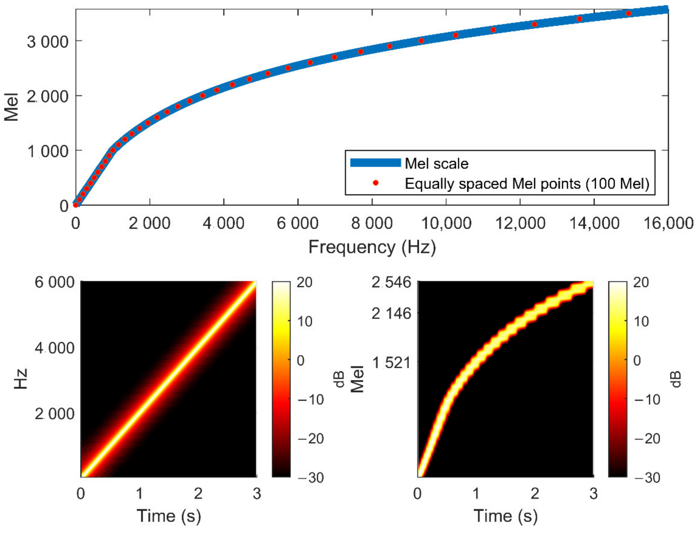
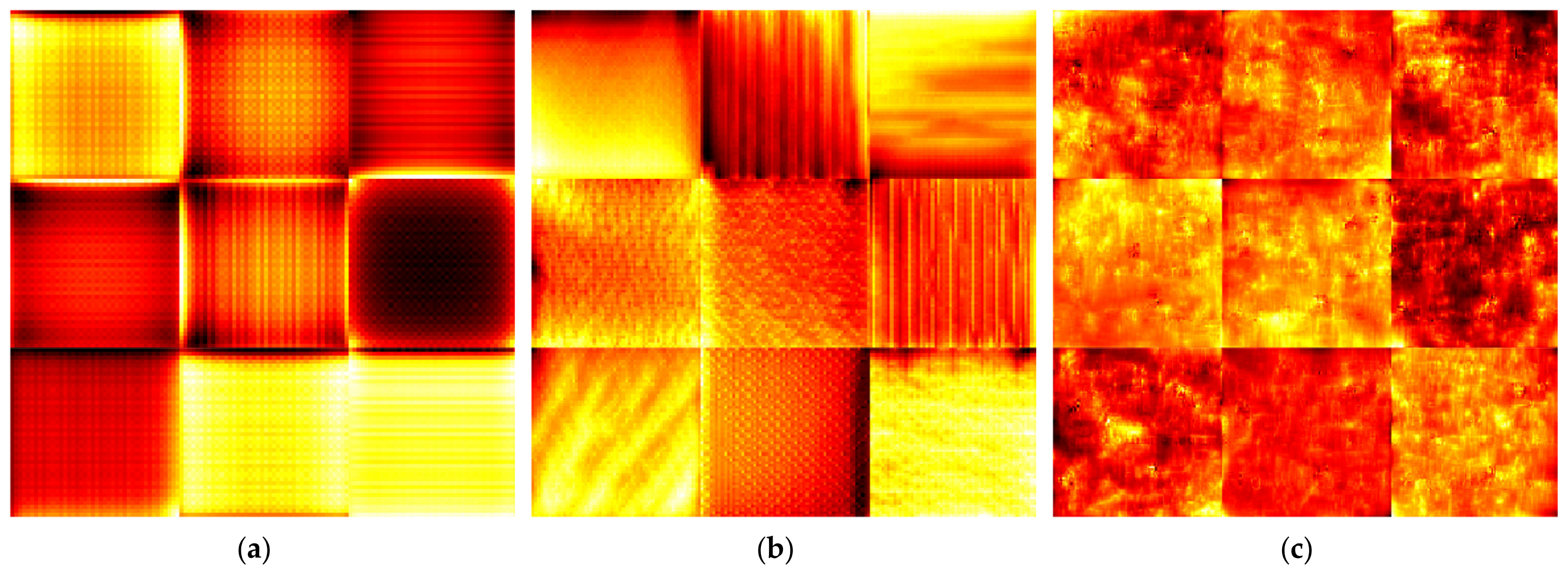
Mel Spectrogram Features

The feature maps that input YAMNet are constructed on the basis of coefficients drawn from time-frequency representations of sounds. However, human perception of sound in terms of frequency content is not linear. It is widely known that humans perceive pitch with better resolution at lower frequency ranges. Indeed, provided a fixed frequency gap between two sounds, our hearing would differentiate tones at lower frequency ranges better than in higher ranges, where tones would seem quite similar. Consequently, artificial intelligences that learn sound perception tasks should account for this aspect. To properly label auditory events, deep learning strategies for speech recognition, music recognition, and SED evolved by exploiting feature spaces pursuant to the human perception of sound. In particular, YAMNet employs a Mel spectrogram feature map.
The Mel (root of the word Melody) scale [60] and the Mel Spectrogram [61] take into account the logarithmic nature of human hearing. The Mel scale is empirically designed on the base of the psychoacoustic perception of pitch. The expression of Equation (3) shows how frequencies f can be converted in M e l :
M e l = f , f 1000   H z 2595   log 10 1 + f 700 , f > 1000   H z
In accordance with human experience, the points that are equally spaced on the Mel scale are not linearly resolved in the Hz scale and vice versa. The Mel spectrogram is a time-frequency representation of sounds, produced by applying Mel scale filter banks to classic spectrograms [61]. Figure 4 shows the Mel conversion curve and reports an example of traditional Hz and Mel scale spectrograms for a linear sine sweep.
Figure 5 shows some of the features extracted from different layers of YAMNet. Compared with AlexNet (Figure 2), the extracted features are distinctive of spectrograms attributes. As previously discussed, this is due to the fact that the weights of YAMNet are specifically optimized to detect spectrograms features. For this reason, the authors of this work hypothesize that some of the knowledge needed to classify REB spectrograms may be already included in the layers of SED networks. This actually means that only the last layers would require learning adjustments, whereas the feature extraction layers and the corresponding weights could be frozen without requiring further training. Then, a small dataset would be sufficient for fine-tuning the net weights, complying with limited data availability.

4. Bearing Fault Detection Using YAMNet and Transfer Learning
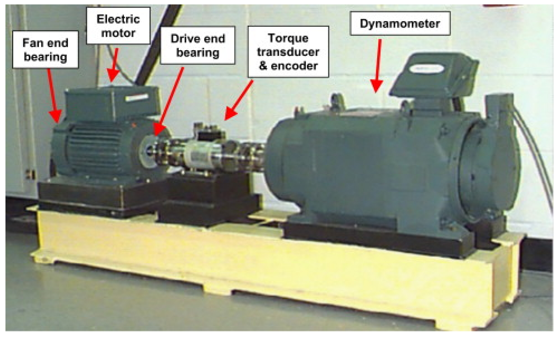
The present work investigates the capabilities of pre-trained SED networks in fulfilling bearing fault diagnosis tasks. Namely, a TL approach was undertaken with the aim of transferring the knowledge held by YAMNet layers to REB spectrograms classification. To this end, the Case Western Reserve University (CWRU) [30,62] bearing dataset was examined, representing a standard reference in this field. The dataset was pre-processed to comply with YAMNet architecture and it was split for training, validation, and test phases. In this context, different labelling options were considered. Afterwards, the network was fine-tuned for dealing with fault diagnosis scenarios characterized by restricted datasets. Finally, the model was tested under new data.

4.1. CWRU Dataset

The CWRU test bench (Figure 6) consists of an electric motor, a dynamometer, and a torque transducer with encoder. Two ball bearings support the motor shaft: one of the bearings (SKF 6205-2RS JEM) is placed on the motor drive end (DE), whereas the other (SKF 6203-2RS JEM) is located at the motor fan end (FE).
The CWRU experimental campaign considered localized faults in DE and FE bearings, which were damaged by means of electro-discharge machining. The faults were introduced separately at the inner race (IR), outer race (OR), and rolling elements (B), and tests were run for motor powers of 0, 1, 2, and 3 hp with a shaft speed ranging between 1721 and 1796 rpm. This study considers the fault diameters of 0.007, 0.014, 0.021, and 0.028 inches for the DE bearing. Vibrations signals were extracted in normal and fault conditions by means of accelerometers placed on the motor housing. In the case hereby examined, normal data were sampled at 48 kHz, whereas DE fault data were sampled at 12 kHz. The OR fault condition with 0.028 in damage was not analyzed since data was not available.

4.2. Dataset Pre-Processing

Three datasets were constructed by rearranging the available vibration signals. Each dataset matched different labelling choices:
  • Dataset A includes 4 classes (B, IR, OR, and Normal);
  • Dataset B includes 12 classes (B007, B014, B021, B028, IR007, IR014, IR021, IR028, OR007, OR014, OR021, and Normal);
  • Dataset C includes 13 different classes (B_0, B_1, B_2, B_3, IR_0, IR_1, IR_2, IR_3, OR_0, OR_1, OR_2, OR_3, and Normal).
The label codification for the dataset B reports the damage type (B, IR, OR) in the first part, whereas the second part denotes the damage severity (007, 014, 021, 028). For example, class IR014 contains signals of experiments run with an inner race damage of 0.014. Dataset C, instead, is labelled using the damage type (B, IR, OR) and the motor load in horsepower (_0, _1, _2, _3). The label OR_3, for instance, indicates that a signal was extracted at 3 hp load with an outer race fault. The network determines the output class by assigning numerical scores at the end of the last layer (classification layer). Given the presence of a Softmax activation function, the output of the last neurons returns the probability of belonging to a certain class. Then, the label of the most likely class is assigned. Essentially, the main difference between the three dataset lies in intra-class distributions. Class B_0 contains samples linked to different damage severities as well as class B007 includes signals extracted at different working loads. Dataset C includes less samples in the OR classes, since data for outer race damages with 0.028 in faults were not available. The CWRU tests were conducted following the labelling of the dataset B; therefore, some class imbalances inevitably occur for datasets A and C. The three datasets were then investigated to have an insight into the effect of different intra-class distributions and imbalances on model performances.
The YAMNet trained model accepts input signals sampled at 16 kHz and normalized in the range 1 ,   1 [56]. Hence, vibration data were pre-processed to fit the model input requirements. Moreover, the similarities between the source and the target domain can be enhanced using Mel spectrum features for vibration signals as well. In so doing, a successful knowledge transfer is more likely to occur. The datasets were randomly split in training (70%), validation (20%), and test (10%) sets, as reported in Table 1. The choice of the dataset split guaranteed the availability of 300 training samples. The training set was employed to fine-tune the model weights, whereas the validation set had the function of monitoring the model convergence and checking potential overfitting issues while training. Finally, the model effectiveness was verified under never-seen data through the test set. It must be pointed out that 300 training samples constitute a very small dataset for such a network, since 2 million AudioSet samples were necessary to properly train the YAMNet deep architecture. Nevertheless, TL leverages on the pre-trained network and provides the opportunity to deal with few data.
As previously mentioned, the effectiveness of the proposed strategy strongly depends on the similarities between source and target domains. Therefore, signals were treated with the same pre-processing that would be carried out for sound event detection. The data pre-processing involves the extraction of the Mel spectrum coefficients for feeding YAMNet architecture, since those coefficients constitute the input feature map. The pre-processing procedure [55,56] provides that:
  • Signals are resampled at 16 kHz and normalized in the range 1 ,   1 ;
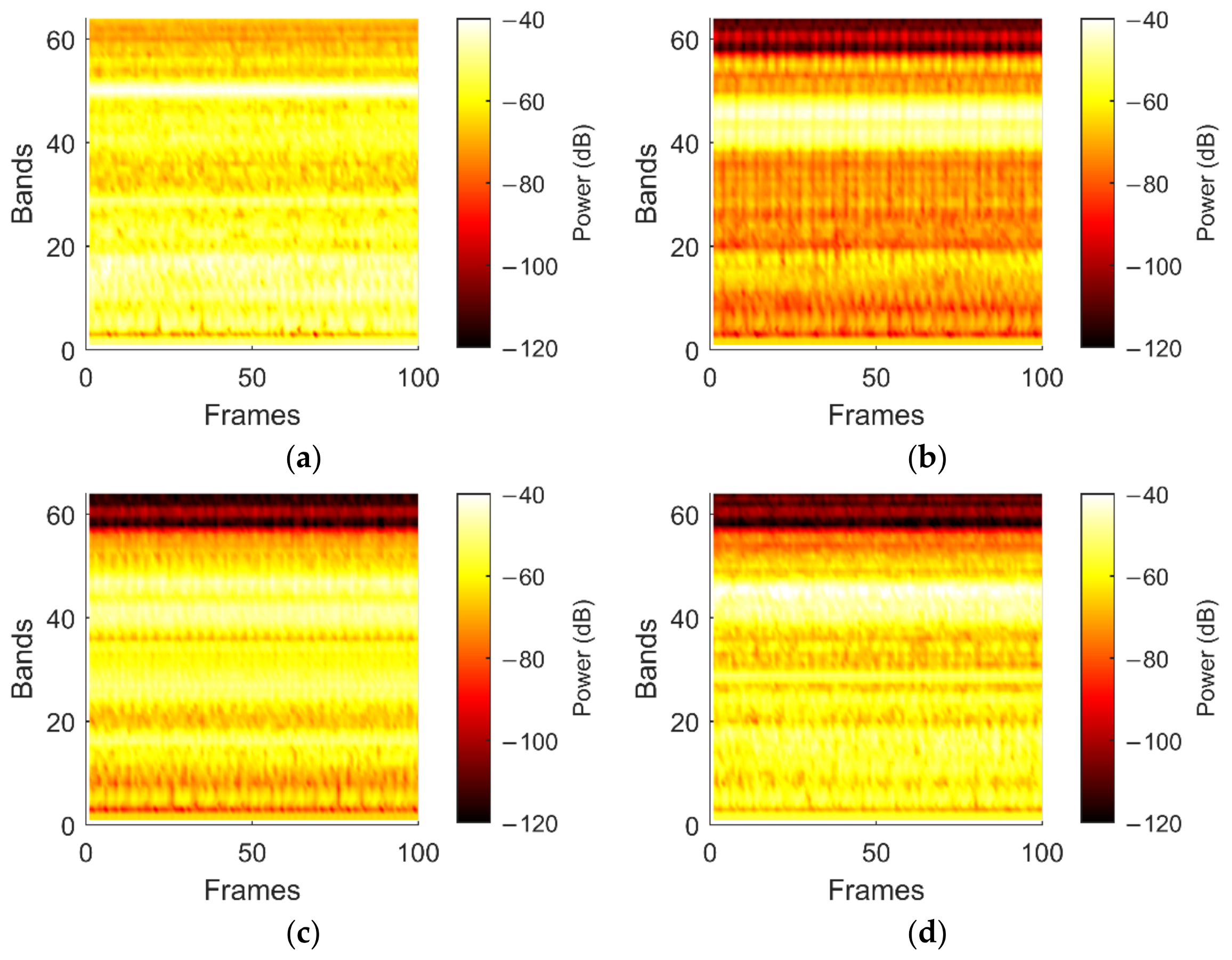
  • The Mel spectrogram is computed using Hann windows with 400 samples length and 60% overlap. The Mel scale filter bank includes 64 filtering bands;
  • The resulting spectrogram is partitioned by using 96 sliding frames with 48 frames of overlap.
In this case, spectrograms lengths resulted of 100 frames and a single 96 × 64 spectrogram was drawn from each signal. Table 2 reports the main features of Mel spectrograms that are consistent with YAMNet architecture. Examples of Mel spectrograms extracted from the CWRU dataset are shown in Figure 7.

4.3. YAMNet Fine-Tuning

It is claimed that the features detectable by the YAMNet framework (Figure 5) provide a source of knowledge to classify bearing spectrograms as well. To verify this assumption, the fully connected and the output layers of YAMNet were replaced with new layers and the convolutional part remained unaltered. The weights of the replaced layers were consequently optimized by training the model with CWRU data. Given the inherent similarities between source and target domains, the replacement of the only fully connected layer was effective. The main hyperparameters featuring the training phase are reported in Table 3.
The Adam optimizer was employed for adapting the learning rate during training [53]. The batch normalization process [59] normalizes mini batches of data for each network channel independently. Such a normalization occurs within layers, thus preventing exploding gradients issues. Over an entire iteration, a mini batch set is passed through the network, whereas a whole epoch involves the complete training set. The validation frequency specifies the number of iterations elapsed between validations. The trend of the loss functions was monitored over the training process. As an example, Figure 8a shows the loss function resulting from training with dataset C.
In this dataset few samples were portioned in a considerable number of classes (Table 1) and overfitting issues manifested. This is evident by the fact that the validation loss remained considerably higher than the training loss. To comply with overfitting matters, a dropout layer with 90% dropout probability was added before the fully connected layer. Dropout layers represent an effective strategy to prevent overfitting in deep networks. Those layers set input elements to zero with a given probability and significantly reduce the number of network parameters. Converge issues can be hypothesized. Figure 8b shows the improvements for network performances due to the dropout layer. A smoother training process is achieved, and overfitting is remarkably mitigated. Training times and epochs are reported in Table 4. For all the datasets, the training stopped either if maximum accuracy was stably reached or if the maximum epochs were met.

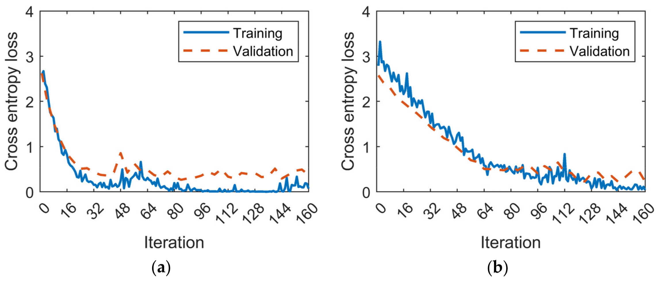
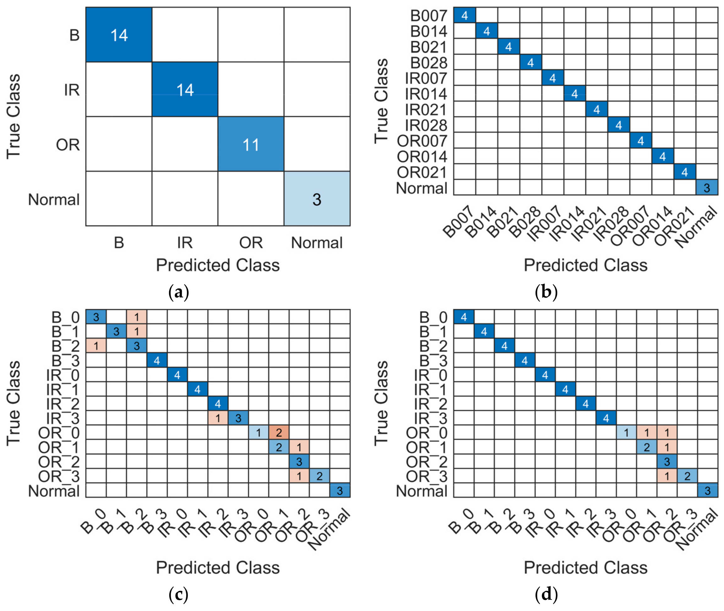
4.4. Model Validation

The fine-tuned model was tested under new data to validate its effectiveness, and the capabilities of TL approaches were assessed in limited data scenarios by leveraging on networks pre-trained with sound events. The confusion matrices resulting from the test data are shown in Figure 9, whereas Table 5 shows the overall accuracies achieved at the end of training, validation, and test. There is evidence that the model can properly perform ideal fault diagnosis tasks for dataset A and dataset B with 100% accuracy. Additionally, no overfitting occurred, though extremely small datasets were employed. The class imbalances associated to data availability for the dataset A did not affect model accuracy. In this sense, the TL strategy was effective when the knowledge of spectrograms features is transferred from an SED network to bearing fault detection tasks. Nonetheless, the replacement of a single layer proved to be adequate because the source domain of YAMNet shared numerous features with the domain of vibration signals, as long as these are properly processed. The adoption of Mel spectrum features is part of the pre-processing, and it enhances similarities between transfer domains. Dataset C showed lower accuracies but, when the dropout approach is applied, performances markedly improved.
The results are consistent with the literature concerning parameter-based TL for CWRU diagnosis. For instance, in [36] it is observed that networks pre-trained on ImageNet are able to perform fault diagnosis tasks with 99.95% accuracy and a training time of 229 s. However, more than one layer required fine-tuning because more training data were available (4000 samples). It can be argued that the dominant features learned on ImageNet were not highly specific of time-frequency images.

5. Discussion

The maximum accuracy is reached when data are split into a considerable number of classes, as long as balanced samples are used (dataset B). Clearly, this is a remarkable capability of TL combined to SED networks, since classes including few more than 20 training samples deliver a very efficient diagnosis model. Training YAMNet from scratch would actually require millions of samples. Similarly, 100% accuracy is achieved also in the event of class imbalances (dataset A), provided that training classes are fed with more training data (Table 1). Interestingly, performances slightly deviate from 100% when class imbalances are superimposed to extremely few training data (dataset C).
Although the accuracy achieved for the dataset C is quite promising, appreciable overfitting occurred in this case, as suggested by the validation and test sets (Table 5). For the diagnosis task of dataset C, training samples did not provide full diagnosis accuracy and the model did not effectively generalize knowledge to new data. Nevertheless, the implementation of a consistent dropout strategy markedly mitigated this effect and remarkable accuracies (higher than 90%) were reached.
Dataset C resulted in a slightly harder form a diagnostic perspective. Contrary to the dataset A, fewer data per class were available and data imbalances affected performances. Depicting intra-class variability at a general level was a harder task for those training data. Indeed, when the dropout improvements are introduced, only the imbalanced OR classes present misclassification (Figure 9d).
Future work can provide a systematic investigation on the performance variations with respect to the size of training sets for such a TL strategy. In this context, weighted loss function can be taken into account to deal with class imbalances. Further, the effect of additive gaussian noise on sample data can be investigated as well. The choice of network hyperparameters can indeed be affected by noisy signals. Automated tuning of hyperparameters is currently a challenging aspect and deserves further improvements. Future research will include additional experimental validation based on different datasets.

6. Conclusions

This study aimed at investigating the capabilities of deep networks pre-trained on sound events in fulfilling bearing fault diagnosis. It is claimed that the inherent knowledge of these architectures in identifying features of audio spectrograms can be transferred to the characterization of machine vibrations as well. For this purpose, transfer learning is applied to an efficient convolutional network. This latter was originally designed to fit AI computing for sound detection in mobile devices. It is concluded that:
  • Networks pre-trained on sound events can fulfill a fault diagnosis task with ideal accuracy by adopting transfer learning approaches;
  • The features learned over stacked convolutional layers of YAMNet architecture are also relevant for spectrograms of machine vibrations;
  • Limited data scenarios can be successfully addressed by replacing a single fully connected layer for fine-tuning YAMNet;
  • When limited data are split in many fault classes with imbalances, overfitting may occur despite high accuracies. In such cases, dropout layers consistently mitigate this phenomenon and further improvements in model accuracies are achieved.

Author Contributions

Conceptualization, E.B., C.D. and L.G.D.M.; methodology, L.G.D.M.; software, L.G.D.M.; writing—original draft preparation, L.G.D.M.; writing—review and editing, E.B. and C.D.; supervision, E.B. and C.D.; project administration, E.B. and C.D. All authors have read and agreed to the published version of the manuscript.

Funding

This research received no external funding.

Data Availability Statement

Publicly available datasets were analyzed in this study. This data can be found here: [https://engineering.case.edu/bearingdatacenter] (accessed on 3 August 2020).

Conflicts of Interest

The authors declare no conflict of interest.

References

  1. Randall, R.B. Vibration-Based Condition Monitoring: Industrial, Aerospace and Automotive Applications; John Wiley & Sons: Hoboken, NJ, USA, 2011; ISBN 9780470747858. [Google Scholar]
  2. Woodley, B.J. Failure prediction by condition monitoring (part 1). Int. J. Mater. Eng. Appl. 1978, 1, 19–26. [Google Scholar] [CrossRef]
  3. Mohanty, A.R. Machinery Condition Monitoring: Principles and Practices; CRC Press: Boca Raton, FL, USA, 2014; ISBN 9781466593053. [Google Scholar]
  4. Liu, R.; Yang, B.; Zio, E.; Chen, X. Artificial intelligence for fault diagnosis of rotating machinery: A review. Mech. Syst. Signal Process. 2018, 108, 33–47. [Google Scholar] [CrossRef]
  5. Lei, Y.; Yang, B.; Jiang, X.; Jia, F.; Li, N.; Nandi, A.K. Applications of machine learning to machine fault diagnosis: A review and roadmap. Mech. Syst. Signal Process. 2020, 138, 106587. [Google Scholar] [CrossRef]
  6. Randall, R.B.; Antoni, J. Rolling element bearing diagnostics-A tutorial. Mech. Syst. Signal Process. 2011, 25, 485–520. [Google Scholar] [CrossRef]
  7. McFadden, P.D.; Smith, J.D. Model for the vibration produced by a single point defect in a rolling element bearing. J. Sound Vib. 1984, 96, 69–82. [Google Scholar] [CrossRef]
  8. McFadden, P.D.; Smith, J.D. Vibration monitoring of rolling element bearings by the high-frequency resonance technique—A review. Tribol. Int. 1984, 17, 3–10. [Google Scholar] [CrossRef]
  9. Antoni, J. The spectral kurtosis: A useful tool for characterising non-stationary signals. Mech. Syst. Signal Process. 2006, 20, 282–307. [Google Scholar] [CrossRef]
  10. Antoni, J. The Spectral Kurtosis of nonstationary signals: Formalisation, some properties, and application. In Proceedings of the 12th European Signal Processing Conference, Vienna, Austria, 6–10 September 2004. [Google Scholar]
  11. Brusa, E.; Bruzzone, F.; Delprete, C.; Di Maggio, L.G.; Rosso, C. Health indicators construction for damage level assessment in bearing diagnostics: A proposal of an energetic approach based on envelope analysis. Appl. Sci. 2020, 10, 8131. [Google Scholar] [CrossRef]
  12. Wang, D.; Tse, P.W.; Tsui, K.-L. An enhanced Kurtogram method for fault diagnosis of rolling element bearings. Mech. Syst. Signal Process. 2013, 35, 176–199. [Google Scholar] [CrossRef]
  13. Hebda-Sobkowicz, J.; Zimroz, R.; Wyłomanska, A. Selection of the informative frequency band in a bearing fault diagnosis in the presence of non-gaussian noise-Comparison of recently developed methods. Appl. Sci. 2020, 10, 2657. [Google Scholar] [CrossRef] [Green Version]
  14. Al-Ghamd, A.M.; Mba, D. A comparative experimental study on the use of acoustic emission and vibration analysis for bearing defect identification and estimation of defect size. Mech. Syst. Signal Process. 2006, 20, 1537–1571. [Google Scholar] [CrossRef] [Green Version]
  15. Mba, D. The use of acoustic emission for estimation of bearing defect size. J. Fail. Anal. Prev. 2008, 8, 188–192. [Google Scholar] [CrossRef]
  16. Al-Dossary, S.; Hamzah, R.I.R.; Mba, D. Observations of changes in acoustic emission waveform for varying seeded defect sizes in a rolling element bearing. Appl. Acoust. 2009, 70, 58–81. [Google Scholar] [CrossRef] [Green Version]
  17. Cortes, C.; Vapnik, V. Support-vector networks. Mach. Learn. 1995, 20, 273–297. [Google Scholar] [CrossRef]
  18. Widodo, A.; Yang, B.-S. Support vector machine in machine condition monitoring and fault diagnosis. Mech. Syst. Signal Process. 2007, 21, 2560–2574. [Google Scholar] [CrossRef]
  19. Yang, Y.; Yu, D.; Cheng, J. A fault diagnosis approach for roller bearing based on IMF envelope spectrum and SVM. Meas. J. Int. Meas. Confed. 2007, 40, 943–950. [Google Scholar] [CrossRef]
  20. Abbasion, S.; Rafsanjani, A.; Farshidianfar, A.; Irani, N. Rolling element bearings multi-fault classification based on the wavelet denoising and support vector machine. Mech. Syst. Signal Process. 2007, 21, 2933–2945. [Google Scholar] [CrossRef]
  21. Zhao, R.; Yan, R.; Chen, Z.; Mao, K.; Wang, P.; Gao, R.X. Deep learning and its applications to machine health monitoring. Mech. Syst. Signal Process. 2019, 115, 213–237. [Google Scholar] [CrossRef]
  22. Krizhevsky, A.; Sutskever, I.; Hinton, G.E. Imagenet classification with deep convolutional neural networks. Adv. Neural Inf. Process. Syst. 2012, 25, 1097–1105. [Google Scholar] [CrossRef]
  23. Guo, X.; Shen, C.; Chen, L. Deep fault recognizer: An integrated model to denoise and extract features for fault diagnosis in rotating machinery. Appl. Sci. 2017, 7, 41. [Google Scholar] [CrossRef]
  24. Lu, C.; Wang, Z.Y.; Qin, W.L.; Ma, J. Fault diagnosis of rotary machinery components using a stacked denoising autoencoder-based health state identification. Signal Process. 2017, 130, 377–388. [Google Scholar] [CrossRef]
  25. Guo, S.; Yang, T.; Gao, W.; Zhang, C. A novel fault diagnosis method for rotating machinery based on a convolutional neural network. Sensors 2018, 18, 1429. [Google Scholar] [CrossRef] [PubMed] [Green Version]
  26. Islam, M.M.M.; Kim, J.M. Automated bearing fault diagnosis scheme using 2D representation of wavelet packet transform and deep convolutional neural network. Comput. Ind. 2019, 106, 142–153. [Google Scholar] [CrossRef]
  27. Wen, L.; Li, X.; Gao, L.; Zhang, Y. A New Convolutional Neural Network-Based Data-Driven Fault Diagnosis Method. IEEE Trans. Ind. Electron. 2018, 65, 5990–5998. [Google Scholar] [CrossRef]
  28. Zhuang, Z.; Lv, H.; Xu, J.; Huang, Z.; Qin, W. A deep learning method for bearing fault diagnosis through stacked residual dilated convolutions. Appl. Sci. 2019, 9, 1823. [Google Scholar] [CrossRef] [Green Version]
  29. Brito, L.C.; Susto, G.A.; Brito, J.N.; Duarte, M.A.V. An Explainable Artificial Intelligence Approach for Unsupervised Fault Detection and Diagnosis in Rotating Machinery. arXiv 2021, arXiv:2102.11848. [Google Scholar] [CrossRef]
  30. Smith, W.A.; Randall, R.B. Rolling element bearing diagnostics using the Case Western Reserve University data: A benchmark study. Mech. Syst. Signal Process. 2015, 64–65, 100–131. [Google Scholar] [CrossRef]
  31. Nectoux, P.; Gouriveau, R.; Medjaher, K.; Ramasso, E.; Chebel-morello, B.; Zerhouni, N.; Varnier, C. PRONOSTIA: An experimental platform for bearings accelerated degradation tests. In Proceedings of the IEEE International Conference on Prognostics and Health Management, Denver, CO, USA, 18–21 June 2012. [Google Scholar]
  32. Daga, A.P.; Fasana, A.; Marchesiello, S.; Garibaldi, L. The Politecnico di Torino rolling bearing test rig: Description and analysis of open access data. Mech. Syst. Signal Process. 2019, 120, 252–273. [Google Scholar] [CrossRef]
  33. Lee, J.; Qiu, H.; Yu, G.; Lin, J. Bearing data set. IMS, Univ. Cincinnati, NASA Ames Progn. Data Repos. Rexnord Tech. Serv. 2007, 38, 8430–8437. [Google Scholar]
  34. Pan, S.J.; Yang, Q. A Survey on Transfer Learning. IEEE Trans. Knowl. Data Eng. 2010, 22, 1345–1359. [Google Scholar] [CrossRef]
  35. Deng, J.; Dong, W.; Socher, R.; Li, L.-J.; Li, K.; Li, F.-F. ImageNet: A large-scale hierarchical image database. In Proceedings of the 2009 IEEE Computer Society Conference on Computer Vision and Pattern Recognition, Miami, FL, USA, 20–25 June 2009; pp. 248–255. [Google Scholar] [CrossRef] [Green Version]
  36. Shao, S.; McAleer, S.; Yan, R.; Baldi, P. Highly Accurate Machine Fault Diagnosis Using Deep Transfer Learning. IEEE Trans. Ind. Inform. 2018, 15, 2446–2455. [Google Scholar] [CrossRef]
  37. Cao, P.; Zhang, S.; Tang, J. Preprocessing-Free Gear Fault Diagnosis Using Small Datasets with Deep Convolutional Neural Network-Based Transfer Learning. IEEE Access 2018, 6, 26241–26253. [Google Scholar] [CrossRef]
  38. Zhang, R.; Tao, H.; Wu, L.; Guan, Y. Transfer Learning with Neural Networks for Bearing Fault Diagnosis in Changing Working Conditions. IEEE Access 2017, 5, 14347–14357. [Google Scholar] [CrossRef]
  39. Hasan, M.J.; Kim, J.M. Bearing fault diagnosis under variable rotational speeds using Stockwell transform-based vibration imaging and transfer learning. Appl. Sci. 2018, 8, 2357. [Google Scholar] [CrossRef] [Green Version]
  40. Li, Y.; Liu, M.; Drossos, K.; Virtanen, T. Sound event detection via dilated convolutional recurrent neural networks. In Proceedings of the ICASSP 2020—2020 IEEE International Conference on Acoustics, Speech and Signal Processing (ICASSP), Barcelona, Spain, 4–8 May 2020; pp. 286–290. [Google Scholar]
  41. Drossos, K.; Mimilakis, S.I.; Gharib, S.; Li, Y.; Virtanen, T. Sound event detection with depthwise separable and dilated convolutions. In Proceedings of the 2020 International Joint Conference on Neural Networks (IJCNN), Glasgow, UK, 19–24 July 2020; pp. 1–7. [Google Scholar]
  42. Hershey, S.; Chaudhuri, S.; Ellis, D.P.W.; Gemmeke, J.F.; Jansen, A.; Moore, R.C.; Plakal, M.; Platt, D.; Saurous, R.A.; Seybold, B.; et al. CNN architectures for large-scale audio classification. In Proceedings of the 2017 IEEE International Conference on Acoustics, Speech and Signal Processing (ICASSP), New Orleans, LA, USA, 5–9 March 2017; pp. 131–135. [Google Scholar] [CrossRef] [Green Version]
  43. Mesaros, A.; Heittola, T.; Virtanen, T.; Plumbley, M.D. Sound Event Detection: A tutorial. IEEE Signal Process. Mag. 2021, 38, 67–83. [Google Scholar] [CrossRef]
  44. Li, Y.; Li, X.; Zhang, Y.; Liu, M.; Wang, W. Anomalous Sound Detection Using Deep Audio Representation and a BLSTM Network for Audio Surveillance of Roads. IEEE Access 2018, 6, 58043–58055. [Google Scholar] [CrossRef]
  45. Butko, T.; Pla, F.G.; Segura, C.; Nadeu, C.; Hernando, J. Two-source acoustic event detection and localization: Online implementation in a Smart-room. Eur. Signal Process. Conf. 2011, 29, 1317–1321. [Google Scholar]
  46. Lee, D.; Lee, S.; Han, Y.; Lee, K. Ensemble of Convolutional Neural Networks for Weakly-Supervised Sound Event Detection Using Multiple Scale Input. DCASE 2017, 1, 14–18. [Google Scholar]
  47. Peng, Y.T.; Lin, C.Y.; Sun, M.T.; Tsai, K.C. Healthcare audio event classification using hidden Markov models and hierarchical hidden Markov models. In Proceedings of the 2009 IEEE International Conference on Multimedia and Expo, New York, NY, USA, 28 June–3 July 2009; pp. 1218–1221. [Google Scholar] [CrossRef]
  48. Gemmeke, J.F.; Ellis, D.P.W.; Freedman, D.; Jansen, A.; Lawrence, W.; Moore, R.C.; Plakal, M.; Ritter, M. Audio Set: An ontology and human-labeled dataset for audio events. In Proceedings of the 2017 IEEE International Conference on Acoustics, Speech and Signal Processing (ICASSP), New Orleans, LA, USA, 5–9 March 2017; pp. 776–780. [Google Scholar] [CrossRef]
  49. Gururani, S.; Summers, C.; Lerch, A. Instrument activity detection in polyphonic music using deep neural networks. In Proceedings of the 19th International Society for Music Information Retrieval Conference, ISMIR 2018, Paris, France, 23–27 September 2018; pp. 569–576. [Google Scholar]
  50. LeCun, Y.; Boser, B.E.; Denker, J.S.; Henderson, D.; Howard, R.E.; Hubbard, W.E.; Jackel, L.D. Handwritten digit recognition with a back-propagation network. Adv. Neural Inf. Process. Syst. 1990, 39, 396–404. [Google Scholar] [CrossRef]
  51. Zhou, P.; Zhou, G.; Zhu, Z.; Tang, C.; He, Z.; Li, W.; Jiang, F. Health monitoring for balancing tail ropes of a hoisting system using a convolutional neural network. Appl. Sci. 2018, 8, 1346. [Google Scholar] [CrossRef] [Green Version]
  52. Yoo, Y.; Baek, J.G. A novel image feature for the remaining useful lifetime prediction of bearings based on continuous wavelet transform and convolutional neural network. Appl. Sci. 2018, 8, 1102. [Google Scholar] [CrossRef] [Green Version]
  53. Kingma, D.P.; Ba, J.L. Adam: A method for stochastic optimization. In Proceedings of the 3rd International Conference on Learning Representations, ICLR 2015—Conference Track Proceedings, San Diego, CA, USA, 7–9 May 2015; pp. 1–15. [Google Scholar]
  54. Guo, L.; Lei, Y.; Xing, S.; Yan, T.; Li, N. Deep Convolutional Transfer Learning Network: A New Method for Intelligent Fault Diagnosis of Machines with Unlabeled Data. IEEE Trans. Ind. Electron. 2019, 66, 7316–7325. [Google Scholar] [CrossRef]
  55. YAMNet Mathworks. Available online: https://it.mathworks.com/help/audio/ref/yamnet.html (accessed on 7 May 2021).
  56. YAMNet Tensorflow. Available online: https://www.tensorflow.org/hub/tutorials/yamnet (accessed on 7 May 2021).
  57. YAMNet GitHub. Available online: https://github.com/tensorflow/models/tree/master/research/audioset/yamnet (accessed on 7 May 2021).
  58. Howard, A.G.; Zhu, M.; Chen, B.; Kalenichenko, D.; Wang, W.; Weyand, T.; Andreetto, M.; Adam, H. MobileNets: Efficient convolutional neural networks for mobile vision applications. arXiv 2017, arXiv:1704.04861. [Google Scholar]
  59. Ioffe, S.; Christian, S. Batch normalization: Accelerating deep network training by reducing internal covariate shift. In Proceedings of the International Conference on Machine Learning, Lille, France, 6–11 July 2015; PMLR. pp. 448–456. [Google Scholar]
  60. Stevens, S.S.; Volkmann, J.; Newman, E.B. A Scale for the Measurement of the Psychological Magnitude Pitch. J. Acoust. Soc. Am. 1937, 8, 185–190. [Google Scholar] [CrossRef]
  61. Rabiner, L.; Schafer, R. Theory and Applications of Digital Speech Processing; Prentice Hall Press: Hoboken, NJ, USA, 2010. [Google Scholar]
  62. CWRU Bearing Data Center. Available online: https://engineering.case.edu/bearingdatacenter (accessed on 3 August 2020).
Figure 1. General architecture of a CNN.
Applsci 11 11663 g001
Figure 2. Examples of features extracted from AlexNet trained with ImageNet data: (a) low-level features; (b) medium-level features; (c) high-level features.
Applsci 11 11663 g002
Figure 3. Pooling operations in CNNs.
Applsci 11 11663 g003
Figure 4. Mel scale (top). Traditional spectrogram (bottom left). Mel spectrogram (bottom right).
Applsci 11 11663 g004
Figure 5. Examples of features extracted from YAMNet trained with AudioSet data: (a) low-level features; (b) medium-level features; (c) high-level features.
Applsci 11 11663 g005
Figure 6. CWRU test bench [30].
Applsci 11 11663 g006
Figure 7. Mel spectrograms drawn from CWRU data: (a) Normal; (b) OR; (c) IR; (d) B.
Applsci 11 11663 g007
Figure 8. Fine-tuning: (a) dataset C; (b) dataset C with dropout layer.
Applsci 11 11663 g008
Figure 9. Test confusion matrices: (a) dataset A; (b) dataset B; (c) dataset C; (d) dataset C with dropout layer.
Applsci 11 11663 g009
Table 1. Dataset split.
DatasetClassesLabelsTraining Samples (70%)Validation Samples (20%)Test Samples
(10%)
A4B1012914
IR1022914
OR762111
Normal2263
Total3018542
B12B0072574
B0142574
B0212574
B0282574
IR0072674
IR0142574
IR0212574
IR0282574
OR0072574
OR0142574
OR0212574
Normal2263
Total2988347
C13B_02574
B_12574
B_22574
B_32574
IR_02574
IR_12574
IR_22574
IR_32674
OR_01953
OR_11953
OR_21953
OR_31953
Normal2263
Total2998247
Table 2. Mel spectrogram extraction for YAMNet architecture.
WindowWindow Length (Samples)Overlap (%)Mel Spectrum BandsMel Spectrum Frames
Hann40060%6496
Table 3. Fine-tuning hyperparameters.
HyperparameterValue
OptimizerAdam
Initial learning rate0.0003
Mini batch size64
Max epochs40
Validation frequency 14
1 An entire epoch corresponds to 4 iterations for the analyzed training sets.
Table 4. Training epochs and training time.
DatasetTraining EpochsTraining Stop CriterionTraining Time (s)
A5 Max accuracy38
B4Max accuracy29
C40Max epochs330
C with dropout40Max epochs330
Table 5. Performances for bearing fault detection using YAMNet and transfer learning.
DatasetTraining AccuracyValidation AccuracyTest Accuracy
A100%100%100%
B98.4%100%100%
C96.9%90.2%83.0%
C with dropout100%93.9%91.5%
Publisher’s Note: MDPI stays neutral with regard to jurisdictional claims in published maps and institutional affiliations.

