Calibration Technique of Thermal Analysis Model for Metal Additive Manufacturing Process Simulation by Nonlinear Regression and Optimization

Abstract

A numerical analysis model that can accurately predict the physical characteristics of the actually additive manufactured products can significantly reduce time and costs for experimental builds and tests. Thermal analysis for the metal AM process simulation requires a lot of analysis parameters and conditions. However, their accuracy and reliability are not clear, and the current understanding of their influence on the analysis results is very insufficient. Therefore, in this study, the influence of uncertain analysis parameters on the thermal analysis results is estimated, and a procedure to calibrate these analysis parameters is proposed. By using the thermal analysis results for parameter cases determined by a design of experiments, a regression analysis model is constructed to estimate the sensitivity of the analysis parameters to the thermal analysis results. Additionally, it is used to determine the optimal values of analysis parameters that can produce the thermal analysis results closest to the given reference data from actual builds. By using the melt pool size computed from a numerical model as reference data, the proposed procedure is validated. From this result, it is confirmed that a high-fidelity thermal analysis model that can predict the characteristics of actual builds from minimal experimental builds can be constructed efficiently.

1. Introduction

Additive manufacturing (AM) is a manufacturing technology that builds a 3D structure from a digital model with a layer-by-layer sequence, and research to apply AM technology to the production of parts is being actively conducted worldwide. In particular, Laser Powder Bed Fusion (LPBF) using metal powder can easily produce parts with a precise and complex structure that cannot be manufactured with conventional manufacturing methods, and it is possible to reduce the weight of parts by topology optimization or lattice structures. Due to these advantages, the use of AM technology is increasing in various industry such as motor vehicles, aerospace, and medical/dental [1]. In order to use the AM manufactured part as an end-use product rather than a prototype in the industry, stability of the material and quality assurance must be guaranteed. For this, it is necessary to accurately predict the characteristics of parts with respect to powder properties and process parameters such as scan pattern, scan speed, and laser power. If the behavior and characteristics of parts can be predicted accurately by a high-fidelity simulation for the LPBF process, time-consuming and expensive specimen or prototype production and testing can be minimized.

For the LPBF process simulation, sequentially coupled thermal-stress analysis is performed, since the stress and deformation fields are affected by the temperature field. Temperature history is obtained by thermal analysis, and residual stress and distortion are predicted by applying temperature history to stress analysis. Therefore, precise thermal analysis must be preceded to obtain accurate and reliable LPBF simulation results. In the LPBF process, metal powders experience a temperature change from room temperature to above the melting point by the laser heat source, so that phase change occurs. In the thermal analysis for the LPBF process simulation, an appropriate heat source model among various heat source models such as a surface Gaussian heat source, a volumetric Gaussian heat source, and a cylindrical shape heat source [2,3] is selected, and phase and temperature-dependent material thermal properties are applied to represent phase changes. Heat dissipation to the environment is considered as boundary conditions such as convection and radiation on the powder surface. However, the analysis parameters such as material properties or thermal coefficients that are used to describe the thermal analysis model for the LPBF process simulation are not only affected by temperature, phase, powder characteristic, etc. but also are difficult to measure accurately. In addition, thermal analysis is generally performed in mesoscopic scale by modeling powder as a continuum without considering in detail complex physical phenomena at the microscopic level such as heat transfer between powder particles, evaporative cooling, and molten metal flow, and this makes the determination of the proper values of analysis parameters more difficult. On the other hand, the effect of these analysis parameters on thermal analysis results such as temperature distribution and melt pool shape has not been fully understood or analyzed. Therefore, this situation leads to limited reliability and accuracy of thermal analysis for the LPBF process simulation.

Many studies related to thermal analysis using FEM have been conducted to simulate the complex LPBF process accurately. Fu et al. [2] performed fully coupled thermal-stress analysis considering multi-layer deposition of Ti-6Al-4V in SLM (selective laser melting) to predict the melt pool shape and dimensions, and they experimentally validated the analysis results. Furthermore, the influence of process parameters and materials on the melting process was evaluated. Zhang et al. [3] performed thermal analysis applying eight heat source models to predict melt pool dimensions and surface features and compared the experimental results to select a suitable heat source model. Afterward, anisotropic thermal conductivity and absorptivity were calibrated by trial and error to increase the accuracy of the simulation. Foroozmehr et al. [4] performed heat transfer analysis by applying a heat source model considering optical penetration depth (OPD) to a finite element model composed of only powder, and the OPD was calibrated and verified by comparing with the experimental value. Ansari et al. [5] analyzed the temperature profile and melt pool size of the powder bed for the SLM process by finite element analysis and compared them with experimental results. Conti et al. [6] evaluated the parameter with the greatest influence on temperature and stress by sensitivity analysis to the physical characteristics of the material (conductivity, specific heat capacity, Young’s modulus). The effects of process parameters (laser power, scan speed, overlap between adjacent paths) on the heat distribution and residual stress of components were evaluated. Dong et al. [7] analyzed the effect of hatching spacing on temperature field, microstructure and melt pool size, overlap rate, surface quality, and relative density by experiments and simulations, and they determined the optimal hatch spacing.

In these studies related to AM process simulations using FEM, several assumptions were made to determine the analysis parameters and conditions. Although the laser heat source penetrates through the powder bed due to the pores between the powder particles, and the penetration depth is determined according to the material and powder characteristics, the penetration depth was simply set to the powder layer [3,6,8,9], or it was assumed that the heat source model did not penetrate through the powder bed and the heat source was applied only to the powder bed surface [2,7,10,11]. In some cases, in order to determine the thermal properties of the powder, porosity was considered [3,4,6,7,8,9,10] or the Marangoni effect causing surface tension in the melting pool was applied [5,8,12]. In some studies [4,10,12], radiation was ignored because it was evaluated to have little effect as a boundary condition. These assumptions reduce the complexity of the finite element model and increase the convergence of the analysis, but the accuracy of thermal analysis with analysis parameter values based on these assumptions cannot be assured for all analysis cases.

In addition to methods using FEM, many studies also have been conducted using CFD and analytical models to propose accurate thermal analysis models for LPBF process simulation and prediction of the melt pool size. King et al. [13] described a multiscale modeling strategy, including a powder scale model that simulated single track/single multi-layer builds and provided powder bed and melt pool thermal data, and the modeling was tied to experiments through data mining. Cheng et al. [14] applied a CFD model to investigate the fluid dynamics in melt pools and resultant pore defects. To accurately capture the melting and solidification process, major process physics, such as the surface tension, evaporation, as well as laser multi-reflection, have been considered in the model. The predicted melt pool dimensions were validated with experimental measurements. Mirkoohi et al. [15] introduced five different heat source models (steady-state moving point heat source, transient moving point heat source, semi-elliptical moving heat source, double elliptical moving heat source, and uniform moving heat source) to predict the three-dimensional temperature field analytically. The proposed temperature field models were validated using experimental measurement of melt pool geometry. Rubenchik et al. [16] determined that the temperature distribution in the simple thermal model of SLM was characterized by two dimensionless parameters (normalized enthalpy and the ratio of dwell time to the diffusion time). In these studies that predict the melt pool size using CFD and analytical models, analysis parameters also have very significant effects on the analysis results, while there are many analysis parameters with high uncertainty. However, there are many difficulties in accurately measuring or determining the values of these analysis parameters.

Although analysis parameters are important factors influencing the analysis results of the models based on FEM or CFD, there are few studies on how accurate and reliable the analysis parameter values are and to what extent they affect the analysis results. In addition, it is also necessary to study how to properly adjust these uncertain analysis parameters to obtain the closest analysis results to the actual builds by LPBF process. Therefore, in this study, the influence of thermal analysis parameters on the analysis results is systematically estimated, and dominant analysis parameters are identified. Furthermore, a procedure for estimating the optimal values of these dominant analysis parameters that can make the thermal analysis model more accurately predict the characteristics of actual products is proposed. This procedure is based on a regression model, which has been utilized in various fields due to its advantages in speed and optimization. To improve the accuracy of the vibration analysis model, a regression model was used [17], and stress was set as a parameter to evaluate fatigue performance [18]. In addition, it was also used to optimize the geometrical and engineering characteristics of building analysis such as tunnels [19], but there was no case applied to the LPBF process simulation. The procedure proposed in this study can be applied to all kinds of analysis models based on FEM or CFD that include uncertain analysis parameters. Through this technique, optimal analysis parameters can be determined more efficiently, and more reliable analysis results even for models with relatively low fidelity can be obtained by applying the optimal analysis parameters. In this study, this technique is applied to a thermal analysis model using FEM.

This paper is organized as follows: Section 2 describes the thermal analysis modeling technique including analysis parameters for the LPBF process simulation using ABAQUS [20], which is a commercial finite element analysis program. In Section 3, a procedure for the estimation of sensitivities and optimal values of analysis parameters by nonlinear regression and an optimization technique is described. In Section 4, the numerical validation of the proposed procedure using reference data generated by thermal analysis models with arbitrary target analysis parameters is carried out. Conclusions and further improvements are given in Section 5.

2. Finite Element Modeling for Thermal Analysis

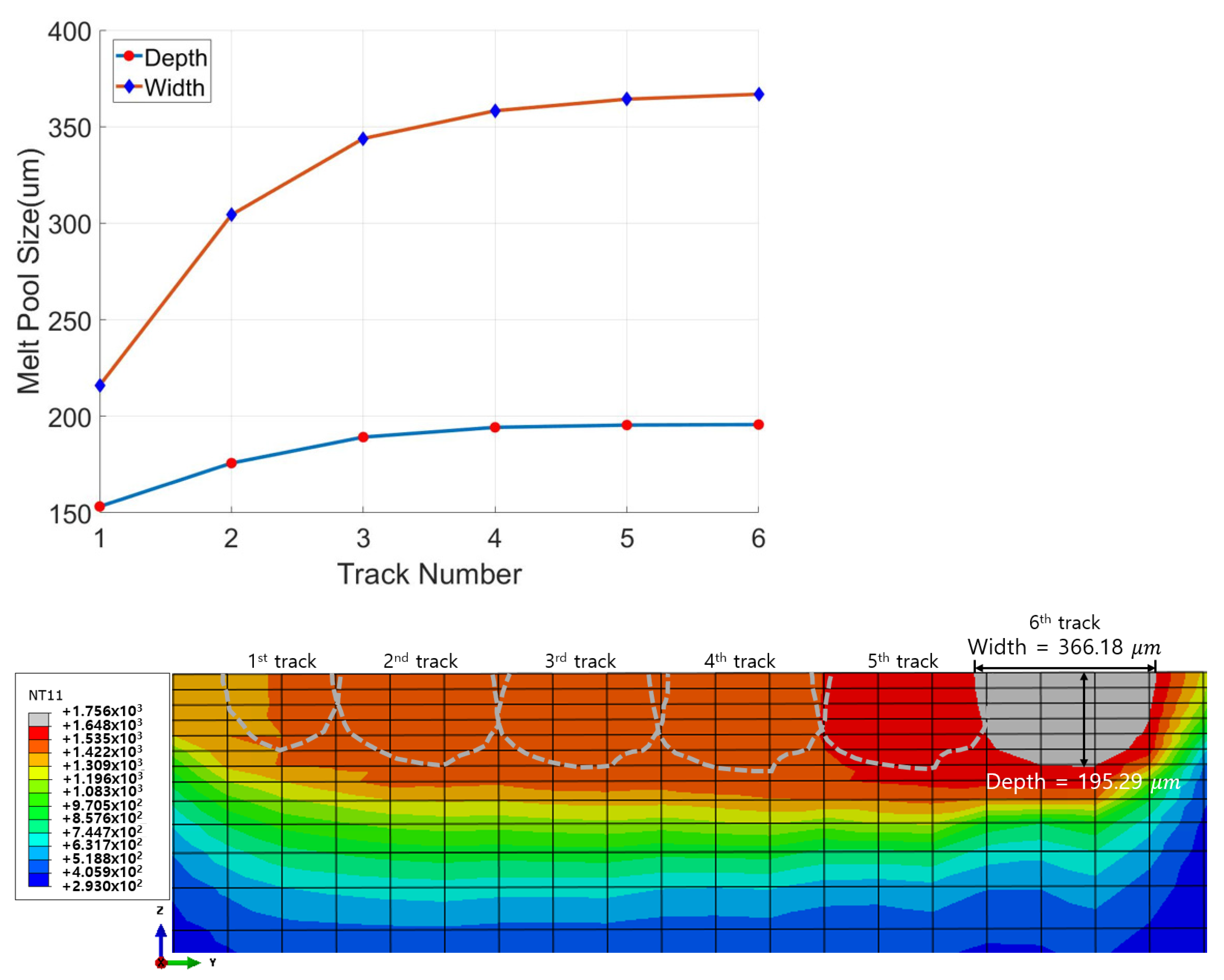
In this research, a high-fidelity thermal analysis model is constructed to conduct precise thermal analysis for the LPBF process simulation using ABAQUS [20]. Figure 1 shows the finite element model and scan strategy, which are used to estimate the melt pool size from thermal analysis. Figure 2 shows the result of the melt pool size with respect to the number of tracks obtained from the test thermal analysis with the process parameters and analysis parameters in

Table 1. Process and analysis parameters used in the analysis of Figure 2.

Parameter		Value
Process parameter	Power (W)	120
	Speed (mm/s)	150
	Radius (mm)	0.2
	Hatch spacing (mm)	0.3
Analysis parameter 1	Convection coefficient $(\mathrm{W}/{\mathrm{m}}^2\mathrm{K})$, $h_c$	10
	Emissivity, $\epsilon$	0.3
	Conductivity coefficient, $\alpha$	0.015
	Porosity, $\phi$	0.4
	OPD, $(\mathsf{\mu }\mathrm{m})$, $H$	140

¹ Descriptions of analysis parameters are given in Section 2.1, Section 2.2 and Section 2.3.

. This test thermal analysis is performed to determine the dimension of the finite element model by identifying the tendency of the thermal analysis results. The result shows that the melt pool size almost converges to a constant after the fifth track. According to Foroozmehr et al. [4], the melt pool size of each track stays almost constant after about 2 mm from the beginning of the track. Considering these, the model is composed of 6 tracks with a length of 3 mm. The dimensions of the model are 5 × 4 × 1 mm, and the dimensions of the scan area where the laser scans the powder bed are 4 × 3 × 1 mm. As shown in Figure 1, 6 lines are sequentially scanned in the x direction, and they are continuously scanned without pause after scanning each track.

According to Roberts et al. [21], if the element size is one-fourth of the laser beam diameter, steep temperature gradients can be simulated sufficiently. Therefore, the element size of the scan area is set to 0.1 × 0.1 mm, and the other regions are filled with coarser elements for computational efficiency. The size of elements in the thickness direction becomes smaller toward the top surface. Considering the thick powder bed and low conductivity of the powder, the base plate is not modeled, and AISI 316L stainless steel powder, which is widely used in the LPBF process, is used as the process simulation material [4].

2.1. Thermal Modeling

The thermal equilibrium equation for 3D heat transfer with isotropic thermal properties is as follows:

$$\rho c\frac{\partial T}{\partial t}=\frac{\partial }{\partial x}\left(k\frac{\partial T}{\partial x}\right)+\frac{\partial }{\partial y}\left(k\frac{\partial T}{\partial y}\right)+\frac{\partial }{\partial z}\left(k\frac{\partial T}{\partial z}\right)+Q\left(x,y,z,t\right)$$

(1)

where $\rho$ is material density ($\mathrm{kg}/{\mathrm{m}}^3$), $c$ is specific heat capacity ($\mathrm{J}/\mathrm{kgK}$), $T$ is temperature ($\mathrm{K}$), $t$ is interaction time ($\sec$), $\mathrm{k}$ is thermal conductivity ($\mathrm{W}/\mathrm{mK}$), and $Q\left(x,y,z,t\right)$ is heat generation per unit volume ($\mathrm{W}/{\mathrm{m}}^3$).

The initial and ambient temperature of the powder bed is set to $293 \mathrm{K}$ ($20 ℃$).

$$T{\left(x,y,z,t\right)}_{t=0}=293 \left(K\right)$$

(2)

As boundary conditions, the side and bottom surface of the FEM model are fixed at $293\mathrm{K}$, and the convection and radiation are considered on the top surface. The convective ($q_c$) and radiative heat losses ($q_r$) are as follows, respectively:

$$q_c=-h_c\left(T_{surf}-T_0\right)$$

(3)

$$q_r=-\epsilon \sigma \left(T_{sur}^4-T_0^4\right)$$

(4)

where $h_c$ is convective heat transfer coefficient ($\mathrm{W}/{\mathrm{m}}^2\mathrm{K}$), $T_{surf}$ is surface temperature ($\mathrm{K}$), $T_0$ is ambient temperature ($\mathrm{K}$), $\epsilon$ is emissivity of the powder bed, and $\sigma$ is Stefan–Boltzmann constant for radiation.

The convective heat transfer coefficient ($h_c$) and emissivity ($\epsilon$) determine the amount of heat release caused by convection and radiation on the powder surface. For sensitivity analysis of thermal analysis parameters, the range of $h_c$ is set from 0, which does not consider convection, to 20 $\mathrm{W}/{\mathrm{m}}^2\mathrm{K}$ [12,22], and the range of $\epsilon$ is set from 0, which does not consider radiation, to 0.66, which is the emissivity of polished steel alloy type 316 at 1222 $\mathrm{K}$ [23].

2.2. Material Properties

In the LPBF process, the powder becomes a liquid state by high energy of the laser and becomes a solid state as it cools. As done by Jeong et al. [24], a global array is created using the UEXTERNALDB user subroutine for ABAQUS, and the temperatures of all integration points are monitored at every increment to check the material phase. Then, phase and temperature-dependent material thermal properties are applied using the UMATHT user subroutine for ABAQUS. Thermal material properties in the solid phase from Mills [25] are used, and the powder properties are determined as follows:

The conductivity of powder is expressed $\alpha$ times the conductivity of the solid, as shown in the following equation. $\alpha$ is the coefficient multiplied by the conductivity of the solid to obtain the conductivity of the powder. The effective thermal conductivity of the metal powder with a diameter of 10–50 $\mathsf{\mu }\mathrm{m}$ is generally 0.1–0.2 $\mathrm{W}/\mathrm{mK}$ at room temperature [2], the conductivity of 316L stainless steel powder is about 0.2–0.25 $\mathrm{W}/\mathrm{mK}$ at 293 $\mathrm{K}$ [26]. Therefore, the range of $\alpha$ is set to 0.0072–0.018 so that the thermal conductivity of AISI 316L powder is 0.1–0.25 $\mathrm{W}/\mathrm{mK}$ at 293 $\mathrm{K}$.

$$k_{powder}=\alpha k_{solid}$$

(5)

As the powder bed is considered as a mixture of solid and gas [4], the density of powder can be written as

$${\rho }_{powder}=\left(1-\phi \right){\rho }_{solid}+\phi {\rho }_{gas}$$

(6)

where $\phi$ is the porosity of the AISI 316L powder bed, which is the ratio of the volume of gas to the total volume of the cell, ${\rho }_{solid}$ is the density of the solid phase, and ${\rho }_{gas}$ is the density of the gas phase. The value of the porosity ($\phi$) ranges from 0 to 1. “$\phi =0$” means the cell only contains gas, and “$\phi =1$” means the cell only contains metal. The porosity ($\phi$) was assumed to be 0.4 in Foroozmehr et al. [4], so the porosity range is set to ±10% based on 0.4 for sensitivity analysis and parameter optimization.

The heat capacity of powder can be written as

$${\rho }_{powder}{C}_{powder}=\left(1-\phi \right){\rho }_{solid}{C}_{solid}+\phi {\rho }_{gas}{C}_{gas}$$

(7)

where $C_{powder}$, $C_{solid}$, and $C_{gas}$ are the heat capacity of the powder bed, solid phase, and gas phase, respectively. In many studies, it was assumed that the heat capacity of the metal powder and the heat capacity of the solid phase were the same [2,4,6,7,9], and it was confirmed by experiments [27].

The material thermal properties of the powder and solid are fitted as a function of temperature as shown in Figure 3 in order to apply in the UMATHT user subroutine.

2.3. Heat Source Model

In the porous material as shown in Figure 4, the laser heat source penetrates through the powder bed and is gradually absorbed along the depth of the powder layer [28]. Therefore, it is important to select an appropriate heat source model in order to simulate the laser heat source of the LPBF process. In this study, the exponentially decaying equation method is applied as a heat source model, and the general form of the exponentially decaying equation method is that the 2D Gaussian distribution is on the top surface while the laser beam is absorbed exponentially along the depth of the powder layer [3]. The intensity of the laser energy at the optical penetration depth (OPD) reduces to $1/\mathrm{e}\left(\cong 37\%\right)$ of the intensity of the absorbed laser beam at the powder bed surface [29]. The specific expression of heat source intensity is as follows and is implemented using the DFLUX user subroutine for ABAQUS.

$$I\left(x,y,z\right)=\frac{2P}{\pi r^2}\exp \left(-2\frac{x^2+y^2}{r^2}\right)\frac{A}{H}\exp \left(-\frac{\left|z\right|}{H}\right)$$

(8)

where $\left(x,y,z\right)$ are coordinates of the center of the heat source, $P$ is power of the stationary laser source, $r$ is the radius of the laser beam, $A$ is laser beam absorptivity, and $H$ is the optical penetration depth (OPD).

The material used in this study is AISI 316L spherical powder with a distribution of average particle size of 45 $\mathsf{\mu }\mathrm{m}$ [4], and the absorption coefficient ($\mathrm{A}$) for this material was found to be 0.52 at scan speeds above 50 $\mathrm{mm}/\mathrm{s}$ [30]. Considering this result, the range of the absorption coefficient ($\mathrm{A}$) is set to ±10% based on 0.52. The OPD ($\mathrm{H}$) of AISI 316L powder can be obtained from the OPD of Ni powder because the absorption of Ni and Fe is in the same range [4,31]. According to experimental investigations of Fischer et al. [32], the OPD in spherical Ni powder with size of 20 $\mathsf{\mu }\mathrm{m}$ is measured to be 20 $\mathsf{\mu }\mathrm{m}$, while it is 200 $\mathsf{\mu }\mathrm{m}$ for the powder size of 50–75 $\mathsf{\mu }\mathrm{m}$. If the OPD for the powder size 50 μm is 170 μm, then the OPD for the powder size 45 μm is calculated to be 170 μm, and if the OPD for the powder size 75 μm is 170 μm, then the OPD for the powder size 45 μm is calculated to be 102 μm by linear interpolation. In this way, the OPD of AISI 316L powder with the size of 45 $\mathsf{\mu }\mathrm{m}$ can be estimated to be in the range of 102–170 $\mathsf{\mu }\mathrm{m}$, and this is set as the range of the OPD ($H$) for sensitivity analysis and parameter optimization.

3. Procedure for Estimation of Optimal Analysis Parameters

A procedure illustrated in Figure 5 is proposed to analyze the effect of thermal analysis parameters on the thermal analysis results and to estimate the optimal thermal analysis parameters for the thermal analysis model to predict the characteristics of actual builds more accurately by using reference data such as melt pool size from test builds. In the first step of this procedure, the ranges of some uncertain thermal analysis parameters are determined considering existing studies and physical conditions as described in Section 2. In the next step, thermal analysis is performed for the analysis cases constructed by design of experiments (DOE) such as Box–Behnken design. The thermal analysis results obtained from the previous step are used to construct a regression model including quadratic terms, and the sensitivity of analysis parameters to the analysis results is evaluated by using this regression model. According to the sensitivity of analysis parameters, dominant analysis parameters are selected for the next step. Finally, for given reference data such as the melt pool size obtained from analysis or experiments for the LPBF process, the optimal values of the selected dominant analysis parameters that can produce the closest thermal analysis results to the reference data are estimated by minimizing the differences between the reference data and the output data from the regression model using efficient optimization techniques such as the particle swarm optimization (PSO) algorithm or the genetic algorithm. By applying the optimal analysis parameters obtained from the optimization step, a thermal analysis model that produces more accurate and reliable analysis results can be constructed. The techniques used in the proposed procedure are briefly described below.

3.1. Design of Experiments

The design of experiments (DOE) is used to efficiently create a regression model using analysis data. The DOE is to select the optimal analysis or experimental cases for the problem to be solved and to plan the experiment. The DOE is a procedure for choosing a set of samples in the design space, with the general goal of maximizing the amount of information gained from a limited number of samples [33].

Factors and levels affecting the results must be determined before designing an experiment with the DOE. In this study, as mentioned in Section 2, factors affecting the thermal analysis results are determined, and the parameter ranges and levels are determined considering the assumptions and physical conditions applied in previous studies. Considering the number of analyses and region of interest, the Box–Behnken design, one of the DOE, is used to construct parameter cases, and then, thermal analysis is conducted for the parameter cases. Figure 6 illustrates the concept of the Box–Behnken design with three factors.

3.2. Multiple Nonlinear Regression

A multiple nonlinear regression model is constructed to mathematically explain the relationship between analysis parameters and output data such as melt pool size obtained from thermal analysis results. A linear regression model including only the first-order terms has limited accuracy in generating a response surface for complex systems such as the thermal analysis model for LPBF process simulation. Therefore, in this paper, the accuracy of the regression model is increased by adding cross-terms and quadratic terms. Response variables (output variables) $Y_1, Y_2, \dots , Y_n$ and regressors (input variables) $X_1, X_2, \dots , X_p$ have the following expression of relation.

$$\mathit{y}=\mathit{\beta }\mathit{X}+\mathit{ϵ}$$

(9)

$$\mathit{y}=\left\{\begin{array}{c}{Y}_1\\ Y_2\\ ⋮\\ Y_{\mathrm{n}}\end{array}\right\},\mathit{\beta }=\left\{\begin{array}{c}{\beta }_1^{\prime }\\ {\beta }_2^{\prime }\\ ⋮\\ {\beta }_{\mathrm{n}}^{\prime }\end{array}\right\}=\left[\begin{array}{cccccccc}{\beta }_{10}& {\beta }_{11}& {\beta }_{12}& \dots & {\beta }_{1,p+1}& {\beta }_{1,p+2}& \dots & {\beta }_{1,2p+\frac{2}{p(p-1)}}\\ {\beta }_{20}& {\beta }_{21}& {\beta }_{22}& \dots & {\beta }_{2,p+1}& {\beta }_{2,p+2}& \dots & {\beta }_{2,2p+\frac{2}{p(p-1)}}\\ ⋮& ⋮& ⋮& ⋮& ⋮& ⋮& ⋮& ⋮\\ {\beta }_{n0}& {\beta }_{n1}& {\beta }_{n2}& \dots & {\beta }_{\mathrm{n},p+1}& {\beta }_{\mathrm{n},p+2}& \dots & {\beta }_{\mathrm{n},2p+\frac{2}{p(p-1)}}\end{array}\right],\mathit{X}=\left\{\begin{array}{c}1\\ X_1\\ X_2\\ ⋮\\ X_1^2\\ X_2^2\\ ⋮\\ X_{11}{X}_{12}\\ ⋮\\ X_{p-1}{X}_p\end{array}\right\},\mathit{ϵ}=\left\{\begin{array}{c}{ϵ}_1\\ {ϵ}_2\\ ⋮\\ {ϵ}_n\end{array}\right\}$$

In this research, $\mathit{\beta }$ represents the sensitivity of the thermal analysis parameters (input variables) influencing output variables such as the melt pool size. As shown in Equation (10), to determine $\mathit{\beta }$, the method of least squares is used, and LASSO (Least Absolute Shrinkage and Selection Operator) regularization is applied to solve the overfitting problem [34]. However, since underfitting may occur with an inappropriate , the method of least squares is used, and LASSO (Least Absolute Shrinkage and Selection Operator) regularization is applied to solve the overfitting problem [34]. However, since underfitting may occur with an inappropriate $\lambda$, k-fold cross-validation is performed to set an appropriate $\lambda$ [34].

$$\mathit{S}={\displaystyle \sum }_{i=1}^n{\mathit{ϵ}}_i^2={\mathit{ϵ}}^{\prime }\mathit{ϵ}={\left(\mathit{y}-\mathit{\beta }\mathit{X}\right)}^{’}\left(\mathit{y}-\mathit{\beta }\mathit{X}\right)+\lambda {\Vert \mathit{\beta }\Vert }_1$$

(10)

In this way, a regression model is constructed using the thermal analysis data for the parameter cases obtained from the DOE, and by analyzing the sensitivity $\mathit{\beta }$, it is possible to determine which thermal analysis parameters have a significant effect on the melt pool size and how large the effect is. The details of the regression model constructed in this study are described in Appendix A.

3.3. Optimization of Analysis Parameters

Given reference data such as the melt pool size obtained from analysis or experiments for the LPBF process, the optimal analysis parameters that can produce the closest thermal analysis result to the reference data can be estimated efficiently by optimization using a regression model. For optimization, the analysis parameters are used as design variables, and the mean square relative error between the output from the regression model ($M{P}_c$) and the reference data ($M{P}_M$) is set as an objective function, which is expressed as follows:

$$\mathsf{\Delta }MP=\frac{1}{N}{\displaystyle \sum }_{i=1}^N{\left(\frac{M{P}_{Mi}-M{P}_{Ci}}{M{P}_{Mi}}\right)}^2$$

(11)

where $N$ is the number of data points, $M{P}_{Mi}$ is the reference value (e.g., the measured melt pool size) at the $i$th position, and $M{P}_{Ci}$ is the output value (e.g., the calculated melt pool size) by the regression model at the $i$th position. The optimal analysis parameters that minimize the objective function are estimated by an optimization algorithm.

Gradient descent, PSO, and Genetic algorithm are used as optimization algorithms to minimize the objective function, and differences due to optimization techniques are compared and verified. These optimization techniques are briefly described below.

The gradient descent algorithm is a technique that moves in the direction of a low gradient, finds the minimum point of the function, and repeats it until the objective function value converges to a specific value [35]. This method may converge to a local minimum depending on the starting point and is expressed by the following Equation (12).

$$x_{i+1}=x_i-\alpha \nabla f\left(x_i\right)$$

(12)

where $x_{i+1}$ is the value of parameter $x$ at the $\left(i+1\right)$th step, $x_i$ is the value of parameter $x$ at the $i$th step, $\alpha$ is the learning rate, and $\nabla f\left(x_i\right)$ is the gradient of objective function $f$ at $x_i$.

The PSO algorithm is a method based on the social behavior of the swarm. Each particle in the swarm moves through the search space, exchanging information with other particles, and moving in a direction set by inertia, cognitive force, and social force to find an optimal solution [36]. This method is expressed by the following Equation (13).

$$\begin{gathered} v_i^{t+1}=w{v}_i^t+c_1{r}_1\left(x^{ind}-x_i^t\right)+c_2{r}_2\left(x^{glo}-x_i^t\right) \\ {x}_i^{t+1}=x_i^t+v_i^{t+1} \end{gathered}$$

(13)

where $v_i$ is the velocity of particle $i$, $x_i$ is the position of particle $i$, $x^{ind}$ is the position of particle $i$ with the lowest objective function among the particles at the current stage, and $x^{glo}$ is the optimal particle position with the lowest objective function during optimization. $r_1$ and $r_2$ are random numbers uniformly distributed in the range [0,1]. $w$, $c_1$, and $c_2$ are the search parameter of the PSO, $w$ is the weight, and $c_1$ and $c_2$ are the knowledge coefficient and social coefficient, respectively.

The genetic algorithm imitates how genetic factors evolve to an optimal state as they pass generations using crossover and mutation. The global optimal solution can be found by repeating the initialization, selection, crossover, and mutation [36].

4. Numerical Validation

In this paper, in order to validate the proposed technique in Section 3, numerical models are used instead of actual experimental data since numerical models are more suitable for quantitative evaluation of accuracy. That is, a numerical model with specific analysis parameter values given is assumed, the melt pool size obtained from the analysis results of the model is used as reference data for the proposed procedure, and then, the accuracy of the proposed procedure can be evaluated by comparing the optimal analysis parameters obtained from the proposed procedure with the original analysis parameters of the assumed numerical model.

Prior to validation, referring to the technical specification of EOSINT M270 equipment, the process parameter cases are set as shown in

Table 2. Process parameter cases.

Case	Power (W)	Speed (mm/s)	Radius (mm)	Hatch Spacing (mm)
1	160	100	0.2	0.3
2	120	150
3	200	150
4	160	200

, and the validation using the numerical analysis model for these process parameter cases proceeds as follows.

4.1. Sensitivity of Analysis Parameters

As mentioned in Section 2, the analysis parameter range is set as shown in

Table 3. Range of analysis parameter.

Analysis Parameter	Min.	Max.
Convection coefficient ($\mathrm{W}/{\mathrm{m}}^2\mathrm{K}$), $h_c$	0	20
Emissivity, $\epsilon$	0	0.66
Conductivity coefficient, $\alpha$	0.0072	0.018
Porosity, $\phi$	0.36	0.44
OPD ($\mathsf{\mu }\mathrm{m}$), $H$	102	170
Absorptivity, $A$	0.468	0.572

. According to the Box–Behnken design to construct a regression model, a total of 54 experiments are performed for six factors, and experiments are repeated six times at the center point. However, since the analysis results are the same at all center points and do not affect the regression model construction, analysis data are generated by performing 49 analysis cases except for duplicated analysis cases at center points.

A regression model is constructed by using the analysis data obtained from these 49 analysis cases. Input variables are normalized values of analysis parameters within the given ranges in Table 3, and the output variables for each analysis case consist of the melt pool depth and width for the process parameter cases listed in Table 2.

Figure 7 shows the sensitivities of the analysis parameters considered for the thermal analysis model, which are the regression coefficients in the regression Equation (9) for normalized values of analysis parameters. As shown in Figure 7, the convection coefficient has the smallest effect on the melt pool size for all process parameter cases, while the porosity, OPD, and absorptivity have significant influences on the melt pool size. Therefore, the porosity, OPD, and absorptivity can be considered as dominant analysis parameters. The emissivity and conductivity coefficient have quite a small effect on the melt pool size for most of the process parameter cases compared with the dominant analysis parameters.

4.2. Regression Model for Parameter Optimization

In order to validate the regression model and optimize the analysis parameters, the parameter ranges are adjusted, and a new regression model is constructed considering the sensitivity analysis results in Section 4.1 and the LPBF process conditions. The convection coefficient, which has a very small sensitivity compared to other parameters, is fixed at 10 $\mathrm{W}/{\mathrm{m}}^2\mathrm{K}$ [4,9,10], and the range of the emissivity is corrected to 0.37–0.45 considering the experimental value of 316L stainless steel powder layer [37]. The conductivity of 316L stainless steel powder at $295\mathrm{K}$ is about 0.2–0.25 $\mathrm{W}/\mathrm{mK}$ [26], so that the conductivity coefficient is set to 0.014–0.018. The OPD range is modified from 120 $\mathsf{\mu }\mathrm{m}$, which is the effective penetration depth in Foroozmehr et al. [4], to 170 $\mathsf{\mu }\mathrm{m}$.

Forty-one analysis cases are generated by Box–Behnken design with the modified parameter range, as shown in

Table 4. Modified range of analysis parameters.

Analysis Parameter	Min.	Max.
Emissivity, $\epsilon$	0.37	0.45
Conductivity coefficient, $\alpha$	0.014	0.018
Porosity, $\phi$	0.36	0.44
OPD ($\mathsf{\mu }\mathrm{m}$), $H$	102	170
Absorptivity, $A$	0.468	0.572

, and a regression model for parameter optimization is constructed. Figure 8 shows the sensitivity for the modified parameter range. The porosity, OPD, and absorptivity have a dominant influence on the melt pool size, while the sensitivity of the emissivity and conductivity coefficient is relatively very small.

For validation of the regression model, three arbitrary analysis parameter cases listed in

Table 5. Analysis parameter case for validation.

Analysis Parameter	Case 1	Case 2	Case 3
Emissivity, $\epsilon$	0.42	0.4	0.38
Conductivity coefficient, $\alpha$	0.017	0.016	0.016
Porosity, $\phi$	0.39	0.41	0.39
OPD ($\mathsf{\mu }\mathrm{m}$), $H$	150	160	130
Absorptivity, $A$	0.57	0.47	0.53

are selected within the parameter range in Table 4. By comparing the melt pool size between the thermal analysis model and the regression model, it can be confirmed whether the regression model accurately traces the thermal analysis model. The melt pool sizes by thermal analysis and the regression model are compared in Figure 9, and the errors are listed in

Table 6. Relative error in melt pool size between analysis model and regression model.

		Process Parameter Case 1	Process Parameter Case 2	Process Parameter Case 3	Process Parameter Case 4
Analysis parameter case 1	Depth	0.18%	0.66%	0.41%	0.59%
	Width	0.61%	1.04%	1.19%	0.34%
Analysis parameter case 2	Depth	2.17%	2.21%	1.82%	2.49%
	Width	1.63%	4.72%	0.13%	0.62%
Analysis parameter case 3	Depth	1.19%	0.14%	0.32%	0.18%
	Width	0.16%	0.81%	0.32%	0.40%

. The largest errors of melt pool depth and width are 2.49% and 4.72%, respectively, but most cases show errors of about 1% or less. Therefore, it can be judged that the regression model has sufficient accuracy to be used for optimization of the thermal analysis parameters for calibration of the thermal analysis model for LPBF process simulation.

4.3. Estimation of Optimal Analysis Parameters

In this paper, six analysis parameters that have uncertain values are considered for sensitivity analysis. However, analysis parameters that have a trivial influence on the analysis results may shift the optimal point significantly, since large changes in these parameters may cause only a small difference in the objective function described in Section 3.3. Therefore, the porosity, OPD, and absorptivity, which are identified as dominant analysis parameters, are selected as design variables for optimization. The reference data to evaluate the objective function of parameter optimization for numerical validation of the proposed method are the melt pool width and depth for all process parameter cases listed in Table 2, which were obtained from the thermal analysis model with each analysis parameter case listed in Table 5. If the melt pool width and depth from actual experimental builds are available, they can be used to evaluate the objective function to find the optimal analysis parameter values for a thermal analysis model that can predict the characteristics of actual builds accurately. The optimization results and errors for the numerical validation cases listed in Table 5 are shown in

Table 7. Relative error in melt pool size between analysis model and regression model.

	Parameter		Gradient	Error (%)	PSO	Error (%)	Genetic	Error (%)
Analysis parameter case 1	Porosity	0.39	0.393	0.8	0.39	0.11	0.39	0.03
	$\mathrm{OPD}(\mathsf{\mu }\mathrm{m}$)	150	152.52	1.68	152.27	1.51	152.36	1.57
	Absorptivity	0.57	0.569	0.18	0.57	0.25	0.57	0.22
Analysis parameter case 2	Porosity	0.41	0.406	0.97	0.41	0.96	0.41	0.96
	$\mathrm{OPD}(\mathsf{\mu }\mathrm{m}$)	160	162.2	1.37	162.14	1.34	162.15	1.34
	Absorptivity	0.47	0.468	0.41	0.39	0.43	0.47	0.42
Analysis parameter case 3	Porosity	0.39	0.393	0.8	0.39	0.73	0.39	0.78
	$\mathrm{OPD}(\mathsf{\mu }\mathrm{m}$)	130	132.23	1.72	132.21	1.7	132.24	1.72
	Absorptivity	0.53	0.531	0.16	0.53	0.2	0.53	0.18

. Errors in Table 7 are the differences between the originally assumed analysis parameter values listed in Table 5 and the analysis parameter values obtained by parameter optimization. As shown in Table 7, three different optimization algorithms converge to similar values with small errors of less than 2% in all cases. Through the numerical validation process as described above, it was confirmed that the analysis parameters of the thermal analysis model that generated the reference data could be estimated accurately using the melt pool size information given as the reference data, and this means that if proper reference data can be obtained from actual experimental builds, a thermal analysis model that behaves similarly to the actual LPBF process can be constructed by using the reference data.

All optimization algorithms used in this study produce similar numerical results, but the number of iterations and elapsed time differ, as shown in

Table 8. The number of iterations and elapsed time according to optimization algorithm.

	Gradient	PSO	Genetic
Number of iterations	254	296,847	495,000
$\mathrm{Time}(\sec$)	0.133	136.61	157.06

. In this case, the gradient descent algorithm seems to successfully converge to a global optimum, and it requires a much smaller number of iterations than other algorithms. However, even for this algorithm, it may take more than 100 h to obtain converged solutions without the regression model, since it takes an average of 2.44 h to perform a thermal analysis once, and 254 evaluations of the objective function are required to complete the iterations. By utilizing the regression model, only 41 cases of thermal analysis need to be performed to complete the parameter optimization; otherwise, thermal analysis should be repeated for every iteration of the parameter optimization, which is almost infeasible.

5. Conclusions

In this study, a new technique to improve the accuracy of the thermal analysis model for LPBF process simulation by nonlinear regression and an optimization algorithm was proposed, and validation was performed by evaluating the errors using a finite element thermal analysis model.

A regression model was constructed using the thermal analysis results for analysis parameter cases generated by Box–Behnken design, and sensitivity analysis and parameter optimization were performed on analysis parameters. According to the sensitivity analysis, it turned out that the porosity, OPD, and absorptivity had a dominant influence on the melt pool size. By applying arbitrary analysis parameter cases for these dominant parameters to the thermal analysis model and using the regression model for validation, it was confirmed that the regression model behaves similarly to the thermal analysis model for the given parameter ranges. By using this regression model, the dominant thermal analysis parameters were optimized so that the thermal analysis model could produce the thermal analysis results closest to the given reference data, which were the melt pool sizes in this study. The optimization results show that the proposed technique can accurately and efficiently find the values of the dominant thermal analysis parameters of the originally assumed thermal analysis model, which has generated the reference data. The thermal analysis parameters obtained by the optimization had a maximum error of 1.72% from the originally assumed analysis parameter values. Therefore, if the proposed technique is applied to the actual LPBF process, it is expected that a high-fidelity thermal analysis model that can accurately predict the characteristics of actual products from the reference data obtained from minimal experimental builds can be constructed efficiently, and this thermal analysis model can significantly reduce the experimental builds required to determine proper process parameters to fulfill quality requirements of additively manufactured products.

References

1. Wohlers Associates. 3D printing and additive manufacturing global state of the industry. In Annual Worldwide Progress Report; Wohlers Associates: Fort Collins, CO, USA, 2021. [Google Scholar]
2. Fu, C.H.; Guo, Y.B. 3-Dimensional finite element modeling of selective laser melting TI-6AL-4V Alloy. In Proceedings of the 2014 International Solid Freeform Fabrication Symposium, Tuscaloosa, AL, USA, 4 August 2014; pp. 1129–1144. [Google Scholar]
3. Zhang, Z.; Huang, Y.; Kasinathan, A.R.; Shahabad, S.I.; Ali, U.; Mahmoodkhani, Y.; Toyserkani, E. 3-Dimensional heat transfer modeling for laser powder-bed fusion additive manufacturing with volumetric heat sources based on varied thermal conductivity and absorptivity. Opt. Laser Technol. 2019, 109, 297–312. [Google Scholar] [CrossRef]
4. Foroozmehr, A.; Badrossamay, M.; Foroozmehr, E.; Golabi, S. Finite Element Simulation of Selective Laser Melting process considering Optical Penetration Depth of laser in powder bed. Mater. Des. 2016, 89, 255–263. [Google Scholar] [CrossRef]
5. Ansari, J.; Nguyen, D.-S.; Park, H.S. Investigation of SLM Process in Terms of Temperature Distribution and Melting Pool Size: Modeling and Experimental Approaches. Materials 2019, 12, 1272. [Google Scholar] [CrossRef] [Green Version]
6. Conti, P.; Cianetti, F.; Pilerci, P. Parametric Finite Elements Model of SLM Additive Manufacturing process. Procedia Struct. Integr. 2018, 8, 410–421. [Google Scholar] [CrossRef]
7. Dong, Z.; Liu, Y.; Wen, W.; Ge, J.; Liang, J. Effect of Hatch Spacing on Melt Pool and As-built Quality during Selective Laser Melting of Stainless Steel: Modeling and Experimental Approaches. Materials 2018, 12, 50. [Google Scholar] [CrossRef] [Green Version]
8. Mishra, A.K.; Aggarwal, A.; Kumar, A.; Sinha, N. Identification of a suitable volumetric heat source for modelling of selective laser melting of Ti6Al4V powder using numerical and experimental validation approach. Int. J. Adv. Manuf. Technol. 2018, 99, 2257–2270. [Google Scholar] [CrossRef]
9. Li, L.; Lough, C.S.; Repogle, A.; Bristow, D.A.; Landers, R.G.; Kinzel, E.C. Thermal modeling of 304 L stainless steel selective laser melting. In Proceedings of the 28th Annual International Solid Freeform Fabrication Symposium, Austin, TX, USA, 7–9 August 2017; pp. 1068–1081. [Google Scholar]
10. Hussein, A.; Hao, L.; Yan, C.; Everson, R. Finite element simulation of the temperature and stress fields in single layers built without-support in selective laser melting. Mater. Des. 2013, 52, 638–647. [Google Scholar] [CrossRef]
11. Xiang, Z.; Yin, M.; Dong, G.; Mei, X.; Yin, G. Modeling of the thermal physical process and study on the reliability of linear energy density for selective laser melting. Results Phys. 2018, 9, 939–946. [Google Scholar] [CrossRef]
12. Ali, H.; Ghadbeigi, H.; Mumtaz, K. Residual stress development in selective laser-melted Ti6Al4V: A parametric thermal modelling approach. Int. J. Adv. Manuf. Technol. 2018, 97, 2621–2633. [Google Scholar] [CrossRef] [Green Version]
13. King, W.; Anderson, A.T.; Ferencz, R.; Hodge, N.E.; Kamath, C.; Khairallah, S.A. Overview of modelling and simulation of metal powder bed fusion process at Lawrence Livermore National Laboratory. Mater. Sci. Technol. 2015, 31, 957–968. [Google Scholar] [CrossRef]
14. Cheng, B.; Loeber, L.; Willeck, H.; Hartel, U.; Tuffile, C. Computational Investigation of Melt Pool Process Dynamics and Pore Formation in Laser Powder Bed Fusion. J. Mater. Eng. Perform. 2019, 28, 6565–6578. [Google Scholar] [CrossRef]
15. Mirkoohi, E.; Seivers, D.E.; Garmestani, H.; Liang, S.Y. Heat Source Modeling in Selective Laser Melting. Materials 2019, 12, 2052. [Google Scholar] [CrossRef] [PubMed] [Green Version]
16. Rubenchik, A.M.; King, W.E.; Wu, S.S. Scaling laws for the additive manufacturing. J. Mater. Process. Technol. 2018, 257, 234–243. [Google Scholar] [CrossRef]
17. Ren, W.-X.; Chen, H.-B. Finite element model updating in structural dynamics by using the response surface method. Eng. Struct. 2010, 32, 2455–2465. [Google Scholar] [CrossRef]
18. Wang, X.; Wang, Z.; Wu, G.; Gan, J.; Yang, Y.; Huang, H.; He, J.; Zhong, H. Combining the finite element method and response surface methodology for optimization of shot peening parameters. Int. J. Fatigue 2019, 129, 105231. [Google Scholar] [CrossRef]
19. Rastbood, A.; Gholipour, Y.; Majdi, A. Finite Element Based Response Surface Methodology to Optimize Segmental Tunnel Lining. Eng. Technol. Appl. Sci. Res. 2017, 7, 1504–1514. [Google Scholar] [CrossRef]
20. ABAQUS. ABAQUS Documentation; ABAQUS, Providence: Johnston, RI, USA, 2012. [Google Scholar]
21. Roberts, I.; Wang, C.; Esterlein, R.; Stanford, M.; Mynors, D. A three-dimensional finite element analysis of the temperature field during laser melting of metal powders in additive layer manufacturing. Int. J. Mach. Tools Manuf. 2009, 49, 916–923. [Google Scholar] [CrossRef]
22. Xing, W.; Ouyang, D.; Li, N.; Liu, L. Estimation of Residual Stress in Selective Laser Melting of a Zr-Based Amorphous Alloy. Materials 2018, 11, 1480. [Google Scholar] [CrossRef] [PubMed] [Green Version]
23. Calex Electronics Limited, “Emissivity Table”. Available online: http://www.calex.co.uk (accessed on 7 September 2020).
24. Jeong, S.H.; Park, E.G.; Kang, J.W.; Cho, J.Y.; Kim, J.H.; Kim, K. Thermal Analysis for Simulation of Metal Additive Manufacturing Process Considering Temperature- and History-Dependent Material Properties. Int. J. Aeronaut. Space Sci. 2021, 22, 52–63. [Google Scholar] [CrossRef]
25. Mills, K.C. Recommended Values of Thermophysical Properties for Selected Commercial Alloys; Elsevier: Amsterdam, The Netherlands, 2002. [Google Scholar]
26. Wei, L.C.; Ehrlich, L.E.; Powell-Palm, M.J.; Montgomery, C.; Beuth, J.; Malen, J.A. Thermal conductivity of metal powders for powder bed additive manufacturing. Addit. Manuf. 2018, 21, 201–208. [Google Scholar] [CrossRef]
27. Badrossamay, M. Selective Laser Melting of Steel Powders. Ph.D. Thesis, University of Leeds, Leeds, UK, 2007. [Google Scholar]
28. Zeng, K.; Pal, D.; Stucker, B. A review of thermal analysis methods in laser sintering and selective laser melting. In Proceedings of the 2012 Solid Freeform Fabrication Symposium, Austin, TX, USA, 6–8 August 2012; pp. 796–814. [Google Scholar]
29. Fischer, P.; Romano, V.; Weber, H.P.; Karapatis, N.P.; Andre, C.; Glardon, R. Modeling of near infrared pulsed laser sintering of metallic powders. SPIE Proc. 2003, 5147, 292–298. [Google Scholar]
30. Badrossamay, M.; Childs, T. Further studies in selective laser melting of stainless and tool steel powders. Int. J. Mach. Tools Manuf. 2007, 47, 779–784. [Google Scholar] [CrossRef]
31. Tolochko, N.K.; Khlopkov, Y.V.; Mozzharov, S.E.; Ignatiev, M.B.; Laoui, T.; Titov, V.I. Absorptance of powder materials suitable for laser sintering. Rapid Prototyp. J. 2000, 6, 155–161. [Google Scholar] [CrossRef]
32. Fischer, P.; Romano, V.; Weber, H.; Karapatis, N.; Boillat, E.; Glardon, R. Sintering of commercially pure titanium powder with a Nd:YAG laser source. Acta Mater. 2003, 51, 1651–1662. [Google Scholar] [CrossRef]
33. Giunta, A.; Wojtkiewicz, S.; Eldred, M. Overview of Modern Design of Experiments Methods for Computational Simulations (Invited). In Proceedings of the 41st Aerospace Sciences Meeting and Exhibit, Reno, NV, USA, 6–9 January 2003; American Institute of Aeronautics and Astronautics (AIAA): Reston, VA, USA, 2003. [Google Scholar]
34. Kolluri, J.; Kotte, V.K.; Phridviraj, M.S.B.; Razia, S. Reducing overfitting problem in machine learning using novel L1/4 regularization method. In Proceedings of the 4th International Conference on Trends in Electronics and Informatics (ICOEI), Tirunelveli, India, 15–17 June 2020. [Google Scholar]
35. Ruder, S. An overview of gradient descent optimization algorithm. arXiv 2016, arXiv:1609.04747. [Google Scholar]
36. Panda, S.; Padhy, N.P. Comparison of particle swarm optimization and genetic algorithm for FACTS-based controller design. Appl. Soft Comput. 2008, 8, 1418–1427. [Google Scholar] [CrossRef]
37. Mohr, G.; Nowakowski, S.; Altenburg, S.J.; Maierhofer, C.; Hilgenberg, K. Experimental Determination of the Emissivity of Powder Layers and Bulk Material in Laser Powder Bed Fusion Using Infrared Thermography and Thermocouples. Metals 2020, 10, 1546. [Google Scholar] [CrossRef]
Figure 1. Finite element analysis model and scan strategy.
Applsci 11 11647 g001
Figure 2. Melt pool size with respect to number of tracks.
Applsci 11 11647 g002
Figure 3. Thermal properties of AISI 316L solid and powder.
Applsci 11 11647 g003
Figure 4. Interaction of laser and powder bed in the SLM process.
Applsci 11 11647 g004
Figure 5. Procedure for estimation of optimal thermal analysis parameters.
Applsci 11 11647 g005
Figure 6. Box–Behnken design.
Applsci 11 11647 g006
Figure 7. Sensitivity of analysis parameters to: (a) melt pool depth; (b) melt pool width.
Applsci 11 11647 g007
Figure 8. Sensitivity of analysis parameters for modified range to: (a) melt pool depth; (b) melt pool width.
Applsci 11 11647 g008
Figure 9. Regression model validation results (melt pool size): (a) analysis parameter case 1; (b) analysis parameter case 2; (c) analysis parameter case 3.
Applsci 11 11647 g009