1. Introduction
The widespread exploitation of wind turbines in mountainous areas or offshore poses issues of limited turbine accessibility and overall cost and complexity of maintenance; furthermore, the relevance of these problems grows as the rotor size increases, as is a recent trend in wind energy technology [
1,
2].
Early detection of gear and bearing damages [
3,
4] is therefore a keystone for improving wind turbine availability and eventually decreasing the cost of energy: for example, in [
5] it is estimated that at least 20% of the non-availability time of a wind turbine is caused by a gearbox failure.
Multi-scale wind turbine monitoring has therefore become a standard in the wind energy practice: recent wind turbine installations are typically equipped of SCADA and TCM control systems. There are remarkable differences in the pros and cons of these two kinds of equipment:
SCADA systems are versatile and provide a bird’s eye view on ambient conditions and on the response of the machine: they typically record and store environmental, operational, thermal, hydraulic variables;
TCM systems are specific: they record vibrations at meaningful mechanical sub-components (gears and bearings);
Industrial SCADA systems record and store the data in the form of average, minimum, maximum and standard deviation in a few minutes sampling time (typically ten);
TCM data have variable sampling times, depending on the target sub-component, and for high-speed rolling elements the millisecond scale (or even less) can be reached;
Upon 10-min averaging, the resulting size of SCADA data sets is manageable and therefore data are recorded and stored continuously;
TCM data are less manageable files and are therefore stored depending on trigger events.
SCADA data are particularly appropriate for analyzing and interpreting wind turbine performance [
6,
7,
8], but are considered to provide late-stage indications of incoming faults. Nevertheless, their simplicity has boosted their diffusion in the industry for real-world applications for, for example, temperature trend analysis [
9,
10,
11,
12].
On the other side, vibration data in general are very powerful for early fault diagnosis but their real-world exploitation is complicated by several issues. Some vibration measurements are integrated into SCADA control systems and their use could be promising in the context of continuous monitoring [
13], but there are important drawbacks regarding the number of channels and the inadequate sampling time. Instead, when employing high-frequency vibration data collected at the sub-components of interest, the most important critical point concerns the difficulty of isolating faulty vibration signatures collected at a type of machine which has a complex gearbox geometry and which operates under severely non-stationary conditions [
14,
15]. For this reason, most of the scientific literature devoted to wind turbine gear and bearing fault diagnosis is based on laboratory tests on components of interest [
16,
17,
18,
19,
20,
21]: few studies [
22,
23,
24] actually deal with the use of measurements collected at wind turbines operating in field.
Another important issue concerns data accessibility: the attitude of private companies to open SCADA data has grown remarkably and there are several accessible data sets for scientific purposes (as in, for example, the Lillgrund test case [
25,
26,
27]). This kind of mentality has not emerged on equal footing as regards TCM data from industrial wind farms: this is also due to the fact that several signal processing techniques require detailed knowledge of the geometry of gearbox [
28,
29,
30,
31], or of other confidential information.
In order to circumvent these issues, in [
32] it has been proposed to diagnose wind turbine bearing faults using vibrations measured at the tower at human height (based on the idea proposed in [
33]). The absence of information about the transfer function from the gearbox to the tower and about the gearbox geometry was compensated for by measuring vibrations simultaneously or nearly simultaneously at the target wind turbine and at reference wind turbines. Extracting meaningful statistical features from the signals processed in the time domain, it was possible to distinguish faulty wind turbines with respect to healthy ones.
This study, similarly to [
32], is a collaboration between the ENGIE Italia company, the University of Perugia and the Politecnico di Torino. The main idea of this work is to analyze only data coming from the industrial SCADA and TCM systems of wind turbines operating in field and the desirable objective is to formulate a methodology for periodically supervising wind farms, which can be integrated into industrial practice.
The combined use of SCADA and TCM data, proposed in this study, is used for practical application on a critical issue which is addressed by many studies in the literature, especially those employing test rig data: the fact that one already knows what component is damaged, independently of the methodology which is formulated in the study. Of course, the scientific method compensates for this upside-down approach with respect to the real-world problem, but the issue remains as regards practical applications: if in wind farm practice one starts from knowing nothing about the health state of a set of wind turbines, it is more complicated to formulate robust methodologies.
On these grounds, the methodology proposed in this study is based on two steps, which use different information sources on different time scales. In summary, it proceeds as follows:
Historical SCADA data are employed for analyzing the wind farm trend of oil filter pressure. This study provides the first consultation about the suspect damaged wind turbines, which are selected as the target in the following step, and identifies the healthy wind turbines, which can be selected as the target. SCADA analysis is then completed with the study of long term trends of temperature measured on the drivetrain components.
TCM vibration data from the selected reference and target wind turbines are analyzed in the time domain, using methods similar to those in [
32], and it is questioned whether there is a statistical novelty of the latter with respect to the former. This kind of result constitutes a basis for damage diagnosis.
It should be noticed that the co-integration of SCADA and TCM data for damage diagnosis is an innovative approach, because typically the former or the latter information source are used separately. A recent attempt has been formulated in [
34], but the point of view is slightly different with respect to the present study. Actually, in [
34], time-resolved SCADA data are employed with the objective of pushing SCADA data analysis to time scales similar to TCM vibration data. The industrial application of the methodology in [
34] is complex and the approach of the present study is instead based on recognizing that the time scale of SCADA and TCM data, which are relatively easily accessible in practice, is intrinsically very different: therefore, in this study it was selected to use them in two steps for different purposes (respectively, first advice and final damage diagnosis).
The test case selected for this study, in collaboration with the ENGIE Italia company, is a wind farm featuring nine Vestas V90 wind turbines, each with 2 MW of rated power: it was selected because of its practical meaningfulness since it is a complex site, characterized by frequent operation under load reduction mode.
Therefore, summarizing, the structure of the manuscript is the following: in
Section 2, the test case and the data sets’ structure are described;
Section 3 is devoted the description of the methods; results are collected in
Section 4; conclusions are drawn and further directions are indicated in
Section 5.
2. The Test Case and the Data Sets
The data used in the present analysis were collected from a multi-megawatt plant located in southern Italy, including of 9 turbines with 2 MW of nominal power each. The three bladed rotor has a diameter of 90 m and has a working range that spans from 4 m/s to 25 m/s of wind speed, where the nominal power is reached at about 12 m/s. This test case wind farm has been considered to be particularly interesting, as its location shows harsh environmental conditions caused by the presence of mountain ridges, gusts and frequent unsteady flow. As a consequence, the wind turbines are frequently subjected to strong solicitations that may cause faults induced by fatigue loads on gearboxes and bearings.
When innovative practices of condition monitoring have to be applied on industrial plants, the low intrusivity of the survey methods plays an important role, as hopefully the collection of data should not influence the energy production. The wind farm object of the study is a valid test case to implement non-intrusive condition monitoring techniques, as it natively includes the measurement of gearbox and nacelle vibrations in its TCM system: the acquired signals can be remotely available for consultation and downloading.
From the turbines a total of 30 signals were acquired, some of which have been used as selection parameters to ensure that the operative conditions were similar among the turbines. In fact, to guarantee the maximum rigorousness of the method, only the time histories at nominal power were included in the analysis.
Other data employed in this study concern quantities providing an overall perspective on the status of the machines, in particular:
Temperature of the main bearing (K);
Temperature of the gear bearing (K);
Temperature of the generator bearing (K);
Oil temperature (K);
Pressures and before and after the filtering of lubrication and cooling oil circuit (bar).
The mentioned quantities all belong to the SCADA system, which in its OPC-DA (Open Platform Communication-Data Access) disposal to the end user have 10 min of sampling time.
To apply a more detailed focus on some significant elements of the turbines, in the present analysis the SCADA data were coupled with TCM ones where vibrations are measured on the bearings and tower with up to 12 KHz frequency. A total of 8 high time resolution signals were acquired that are comprehensive of:
Nacelle accelerations in the Fore–Aft,Side–Side and vertical directions (NacXdir, NacYdir, NacZdir);
Main bearing rear and front side (MnBrgRr,MnBrgFr);
Gearbox high speed shaft rear and front (GbxHssRr,GbxHssFr);
Intermediate shaft speed (GbxIss).
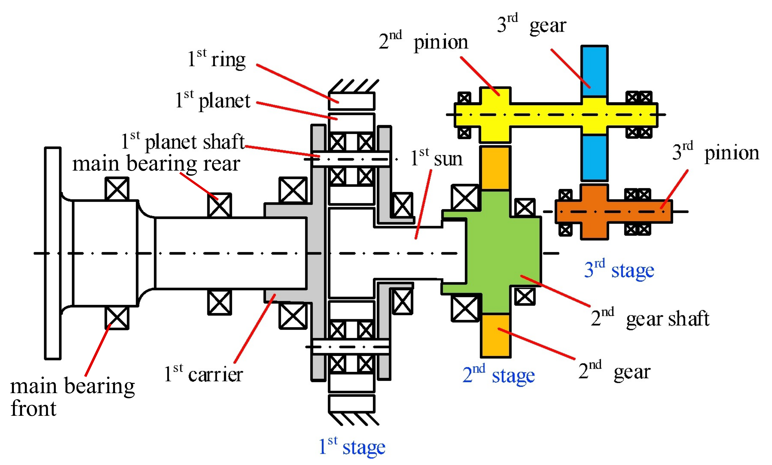
The general gearbox layout is represented in
Figure 1: this is the typical three stages gear used in multi-MW machines with the input planetary stage and two parallel stages.
3. Methods
In the present paper, 2 wind turbines belonging to the previously described site were analyzed during a period between January 2020 and May 2021.
Turbine T04 was considered the healthy reference, as during this period no faults or damages were recorded by the supervision systems. The second turbine (T02), instead, was subject to damage on the main bearing in late August 2020, when it was stopped for maintenance until January 2021. The procedure for the predictive condition monitoring based on SCADA and TCM data, explained in the following sections, was applied to both turbines T.Ref (the healthy T04 turbine) and T.Tar (the faulty T02 unit) with the aim of keeping the healthy Reference machine as the control reference while monitoring the progression of the damages on the faulty Target one. In the end, the method was double-validated on the first months of 2021 when the main bearing of T.Tar had been fixed. The main issues of SCADA and TCM data, that this study aims to overcomes, concern the forecasting and the localization of damages. A method of condition monitoring can be considered reliable and efficient when it is able not only to advice a possible fault with sufficient advance, in order to timely plan the maintenance procedures, but even to define in good detail the mechanical element that has been affected by the malfunction.
For this reason, it is necessary to consider in condition monitoring practice the highest possible types of data sources, possibly with different time scales, and different methods of processing. As will be shown in the following section, a first overall overview on the status of the turbines can be produced by processing raw SCADA data, with a quite simple approach. In spite of this, this preliminary analysis should be supported by a more detailed and consistent examination in order to detect the precise localization of the fault.
3.1. SCADA Data Analysis
One of the most meaningful indicators about the general status of the machine is the delta pressure (
) between the filter of lubrication and cooling oil circuit. This parameter is constantly monitored by the SCADA system and was included in the analysis as it can be useful to ascertain the presence of a possible fault, coming from an abnormal erosion of some mechanical parts, i.e., pitting phenomena, and causing the accumulation of metallic debris on the oil filter whose presence can be quantified by the
given in Equation (
1):
where
is the pressure of the oil before the filter and
is the pressure after the filter. In
Table 1 the average values of
are summarized for each turbine for the period before the gearbox maintenance on T02 (from January to August 2020) and the period after the maintenance (from February to May 2021).
The values of were averaged on a daily basis to analyze the trend for the faulty turbine T02 (T.Tar in the following) and compare it with the trend of the chosen reference healthy unit T04 (T.Ref). The SCADA system can also gather signals from temperature sensors that are dislocated in multiple points of the gearbox and, more in general, all over the main components of the turbines. In combination with , the temperature sensors are expected to provide more detailed information about the localization of the faulty element.
The main possible drawback of the previously described approach concerns the possibility that from the raw temperature signal it might be non-trivial to find a clear evidence of the damage, as temperatures tend to increase noticeably only when damages are fully developed. For this reason, a processing of the temperature data is proposed in the present paper through the use of support vector regression(SVR), which is described in the following subsection.
3.2. Support Vector Regression
The Support Vector Regression is inspired by classifications problems, i.e., the determination of the best line (or hyperplane, in multiple dimensions) demarcating observations. Subsequently, a regression based on these principles was formulated and widely used in data analysis, especially for facing non-linear problems. For details, refer for example to [
36].
In its linear form, Support Vector Regression is a constrained optimization problem, whose objective function contains the potentially conflicting targets of minimum norm of the coefficients vector (which means flatness) and residuals between the measurement and model estimate being lower than a threshold for each observation.
In practice, if
is the matrix of observation and
y is the target, for a linear model the function to minimize by selecting appropriate Support Vectors
and
is given in Equation (
2):
with the constraints (Equation (
3))
C is called the box constraint and it is a hyperparameter of the model, quantifying the cost of misclassified points: the higher the box constraint is, the higher the cost of misclassification is, and this leads to a better separation of the data.
Referring to classifications problems, it can happen that the observed data cannot be easily classified as they are, but they become classifiable if transformed to a feature space, where for feature space it has to be intended as a higher dimensional space where the linear separation is possible. This idea is at the basis of the non-linear Support Vector Regression, which is obtained by replacing the scalar products between the observation matrix of Equation (
2) with a non-linear Kernel function (Equation (
4)):
where
is a transformation mapping the
observations into the feature space.
A Gaussian Kernel selection is given in Equation (
5), where
is the kernel scale:
Once the model has been trained, it can be used for predicting the output, given the input
, using Equation (
6):
If the data are non-standardized, it is necessary to add into Equation (
6) a constant shift
b which has the same meaning as the intercept in a linear model.
The critical points regarding the application of Support Vector Regression are the optimization of the hyperparameters and the input variables’ selection.
As regards the former, the typical approach is fixing a certain number of model runs and, for each run, one hyperparameter at a time is varied randomly in a selected range. The data are divided in certain proportions (training and test) and the best configuration is selected by targeting a loss function (an error metric) to minimize for the test data set. For this study, the Root Mean Square Error was selected, which is given in Equation (
7):
where
M is the number of samples in the test data set and
is the mean error, defined in Equation (
8):
The input variables’ selection is dictated by the kind of problems to which the regression is applied. In the case of anomaly detection, the input variables should be strongly correlated with the target because the interest is in having a reference on the expected value of the target. When the other way round, they should not be so correlated as to contain practically the same information as the target, because this would not help in highlighting the novelty hidden in the target measurements, which is given by the fault.
For each target
y, the most appropriate input independent variables of the model were checked by constructing a cross-correlation map basing on the Pearson correlation coefficient (Equation (
9)) with each possible regressor
x:
where
N is the number of observations in the training data set,
and
are the averages of the output and of the potential regressor
x in the training data set. The selected regressors are required to have
with the target between 0.4 and 0.98. The final choice was to keep fixed inputs with different predicted outputs: for boosting the sensitiveness of the approach only machine parameters and the ambient temperature were used to predict the temperature of the different components of the drivetrain. The ambient temperature was included to correct the bias due to seasonal variability; anyway, the contribution of this parameter was discovered to be marginal in improving the reliability of the analysis.
The selected input variables and output are finally reported in
Table 2.
The flow chart in
Figure 2 resumes the methodology used for the processing of the SCADA data: oil pressure and temperatures were, at first, studied with weekly averages where general information about the status of the machines was retrieved (presumably faulty or healty). Then, a more specific analysis with machine learning approach was applied, modelling the trend of temperatures.
3.3. TCM Data Analysis
The TCM data consist of acquisitions from accelerometers placed on the gearbox casing. Such acquisitions are triggered by “events”, hence they can be quite noisy or display operational adaptation to different work conditions. A pre-processing is then needed to treat the data. In this case, the idea was to first extract traditional time features such as RMS, skewness, kurtosis, peak value and crest factor (i.e., peak/RMS), and then identify outliers in such feature space. Univariate outliers can be evaluated using a Hampel filter based on the median absolute deviation MAD [
37,
38]. A sample
that falls out of the confidence interval:
is then considered an outlier and is substituted with the median value along the analyzed window. The parameter
K is commonly set to 3, similarly to the well-known
rule but for the present analysis a value of
was selected to identify the variability due to non-stationary operational conditions of the wind turbine. Furthermore, being the features of different orders of magnitude, these were standardized according to a mean value
and a standard deviation
computed on the training set alone. Finally, a Novelty Detection based on the well-known Principal Component Analysis (PCA) was used. From a mathematical point of view, PCA corresponds to the solution of the eigenproblem based on the covariance matrix
S of the preprocessed dataset
X (i.e.,
). Therefore, for example, taking just the first principal direction corresponds to projecting the original multivariate space onto the direction of the first eigenvector
[
39]. From an example reported in
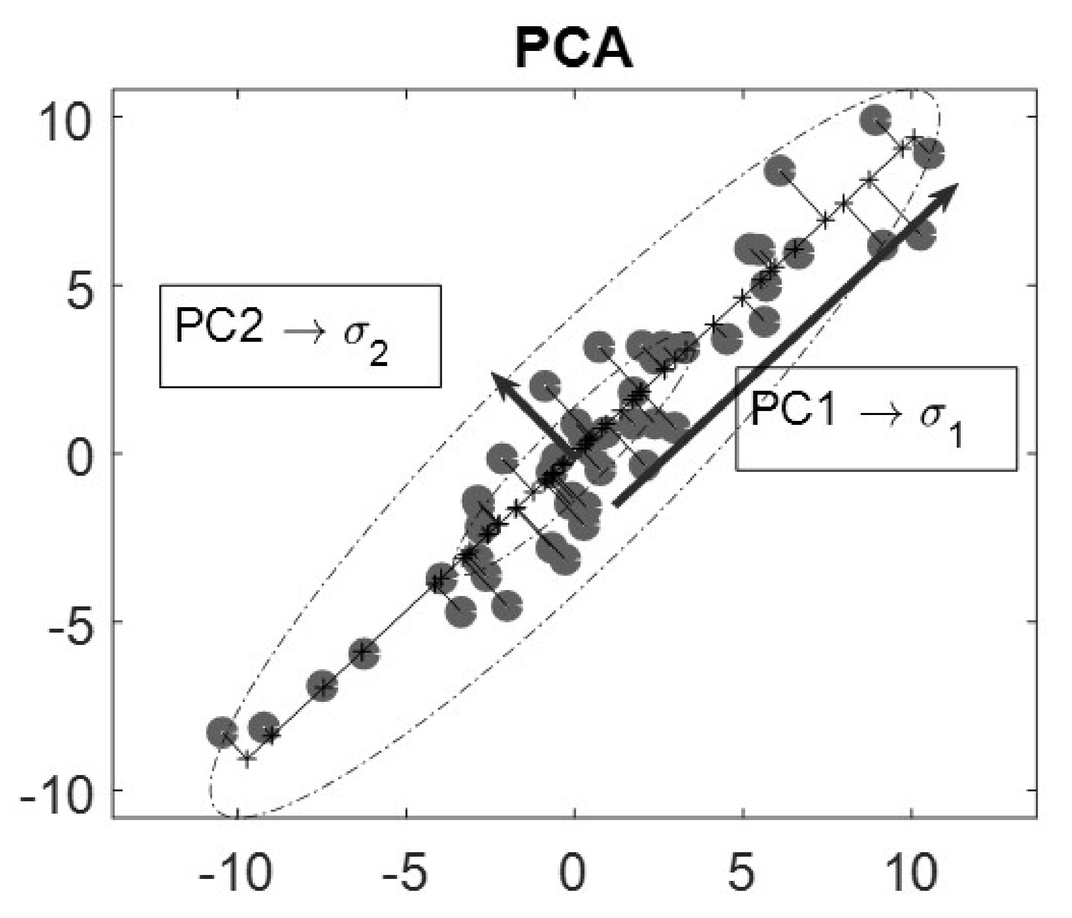
Figure 3, the added value of PCA can be appreciated: this is given by the fact that a raw data set might not have remarkable patterns, but these might arise once the data set has been projected on the principal components. For example, in
Figure 3 it can be seen that the data tend to adapt to a straight line in the plane constituted by the first two principal components.
The so defined Novelty Index is then a linear combination of the original features able to pursue a dual purpose: the dataset is further compressed to a 1D information, while a pattern recognition is achieved, as the damage information is highlighted.
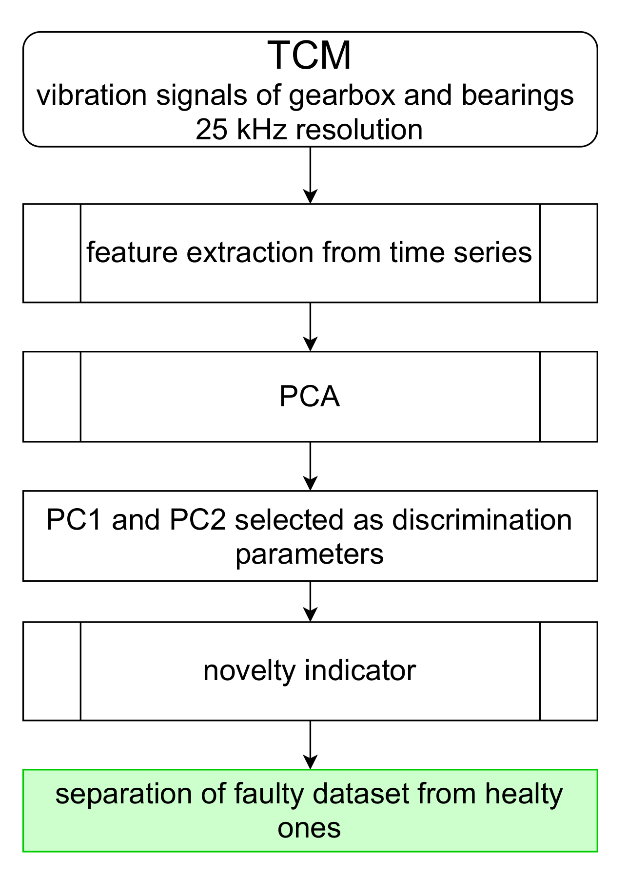
A sum up of the TCM analysis is presented in
Figure 4 where all the steps of the processing of the vibrations signals are shown.
4. Results
4.1. SCADA Data Analysis
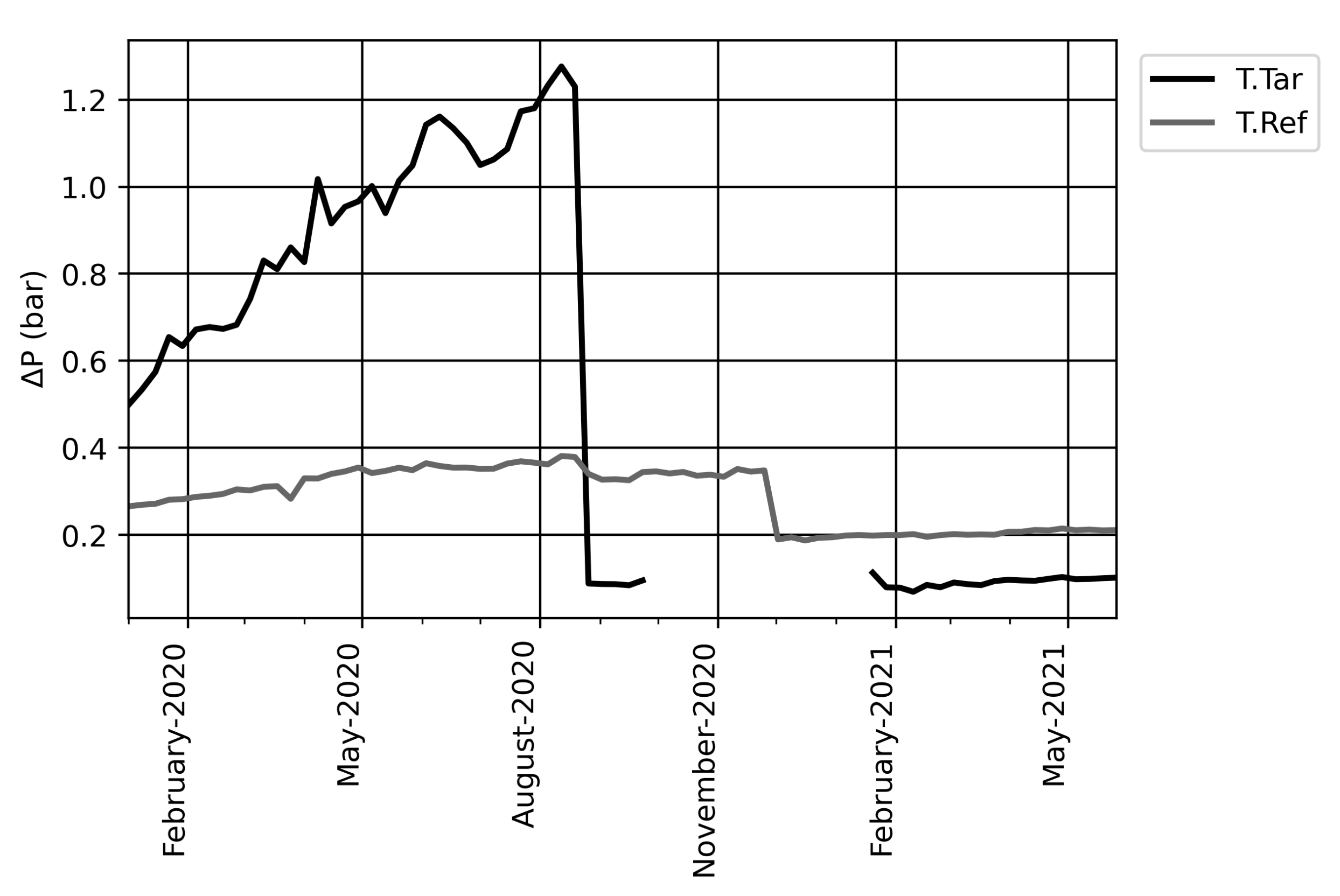
Figure 5 shows the
of the two considered turbines, T.Ref (reference) and T.Tar (faulty). Considering that the curves are computed as the one week mean value of the
, it can be seen that the progression of the damage is clearly visible in the faulty wind turbine even with a forewarning in the order of six months, confirming that this parameter can be considered a valuable indicator by the point of a preventive condition monitoring strategy. In spite of this, the possibility to uniquely identify the origin of the fault is still lacking as the single lubricating oil circuit serves multiple mechanical components, and so, considering only the
of its filter, it is still not possible to find the source of the debris, and, as a consequence, the faulted element.
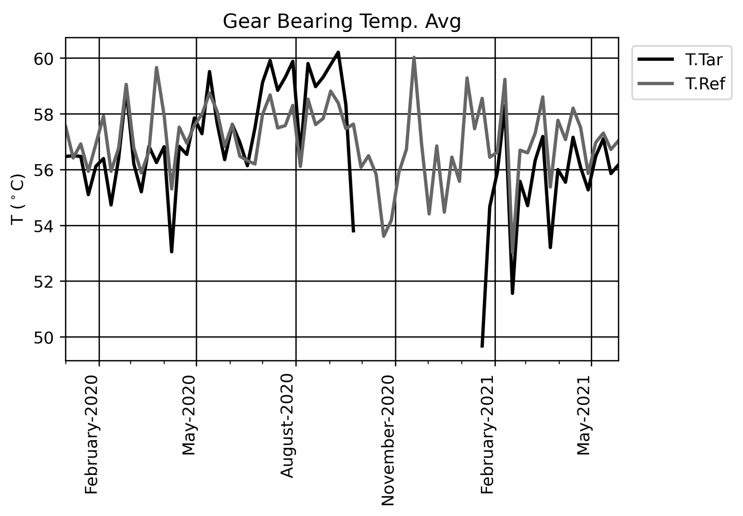
For this purpose, the temperature sensor signals are included in the analysis: as can be seen in
Figure 6, the raw data of temperatures from SCADA do not allow a clear identification of the fault, as no visible differences can be found between the reference turbine and the faulted one. If the percentage difference is taken into account, its maximum reaches the value of about 3% on the two months before the fault, which cannot be considered a valuable threshold to detect the damage: such a low difference may even be ascribed to external random variability, as the turbines may have slightly different environmental or operative conditions.
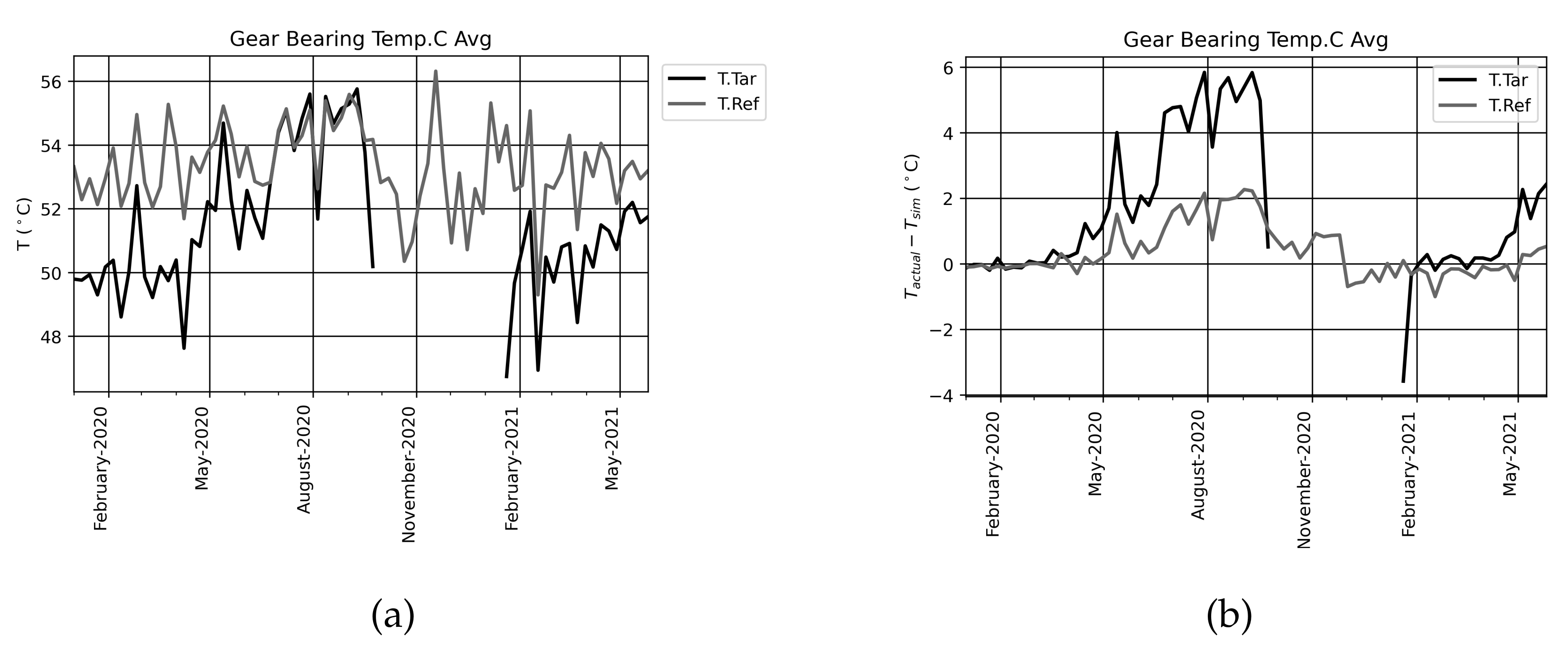
Applying the SVR method to the temperature SCADA data, it becomes possible, at first, to amplify the differences between the healthy and the faulty turbines. In
Figure 7 the differences between the actual “Gear Bearing” temperature and the simulated one are represented. Thanks to this method, the variability introduced by environmental or operational conditions becomes less influential, as the value of the error
is computed separately for each turbine and it can only be ascribed to a different behavior of the real turbine with respect to the simulation obtained by the trained model. A positive drift of the error represents a clear symptom of the heating of the component due to an incoming fault. It is also noticeable to consider, in addition, that in the period May 2020–July 2020 the raw SCADA do not show any anomaly, while the SVR-processed data are able to identify an incipient fault, as the differences between the two curves are still limited but an increasing trend is visible.
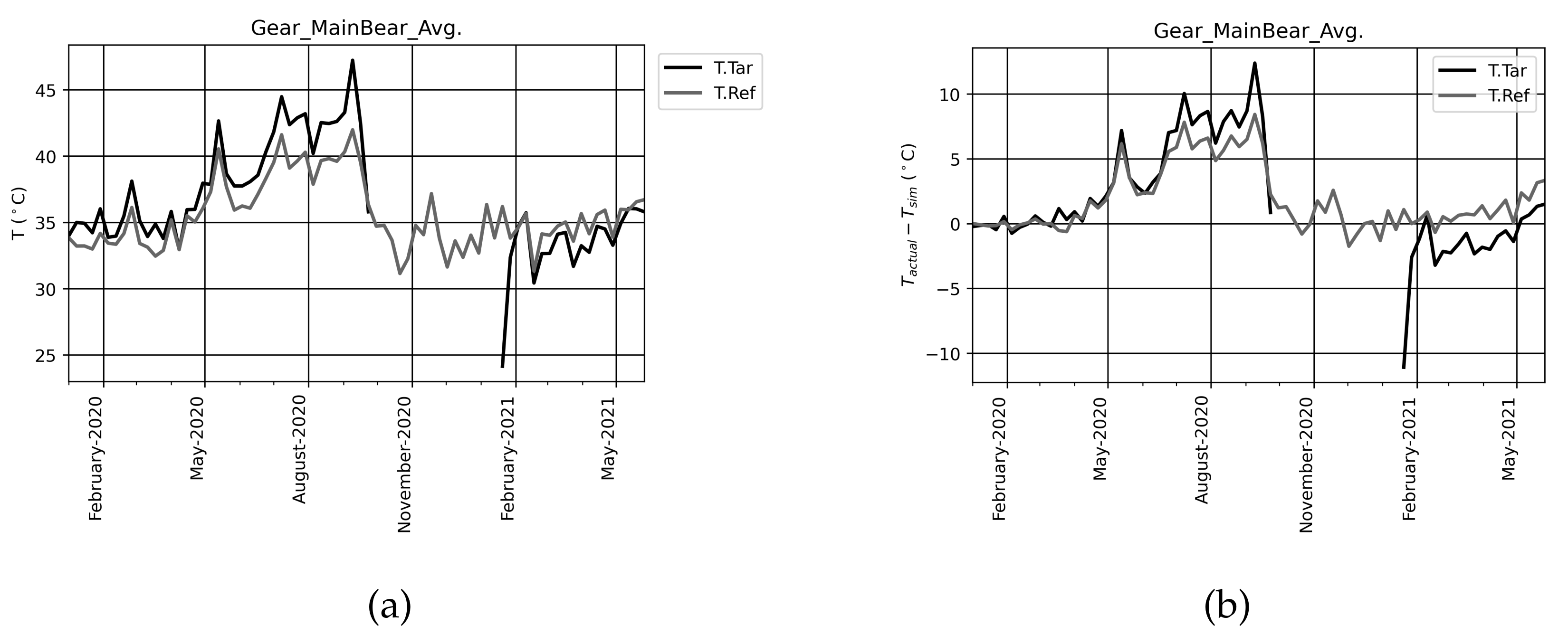
This kind of behavior was observed only on the temperatures measured near the gear. The most responsive temperature channel was the gear bearing C (see
Figure 7), which is the last bearing supporting the gear on the second stage as the shaft input the power to the high speed parallel stage (see
Figure 1). Any advice of the incoming fault was discovered on the generator bearing or the main bearing (
Figure 8) supporting the slow input shaft.
The trend of the error of the SVR model for the gear bearing temperature is able to isolate the faulty drift four months before the turbine stops. In light of the fact that the model was trained using the data of the first three months of 2020, this can be considered a valuable result. After the maintenance the error of the SVR assumes a trend similar to that of the healthy reference units; this confirms the applicability of the approach for fault detection.
4.2. TCM Data Analysis
In order to test the effectiveness of vibration sensors for diagnostics, TCM data for the beginning of 2020 were selected to be compared with data for the beginning of 2021. In fact, given that at the end of 2020 T.Tar underwent an extraordinary maintenance intervention, the incipient damage could be visible in such data. T.Ref turbine data were added to validate the method and increase the statistical confidence of the analysis.
A total of four acquisitions at nominal conditions were chosen (i.e., rpm, MW, see
Table 3), each of them involving seven uniaxial accelerometers MnBrgRr, MnBrgFr, NacXdir, NacZdir, GbxHssRr, GbxHssFr, GbxIss sampled at 25.6 kHz for about 10 s. This dataset was processed according to [
40,
41,
42]. In particular, each signal was divided into 100 chunks of
s each, and 5 time feature was extracted (i.e., RMS, skewness, kurtosis, crest factor, peak value). Every acquisition was then turned into a matrix of 100 rows by 35 columns (7 channels, 5 time-features). First, the data were pre-processed by removing univariate outliers using a Hampel filter of a size of 10 samples. Then, a second univariate pre-processing followed. Each feature of the outlier-free dataset was standardized by removing the mean value and dividing by the standard deviation, and computed on the training set alone. The previously proposed multivariate Novelty Detection algorithm was finally implemented on the pre-processed dataset to quantify the novelty in the acquisitions, i.e., the distance of a sample from the reference healthy distribution. Given the stationarity of the acquisitions (i.e., nominal speed and power, see
Table 3) novelty can be easily related to the presence of damage [
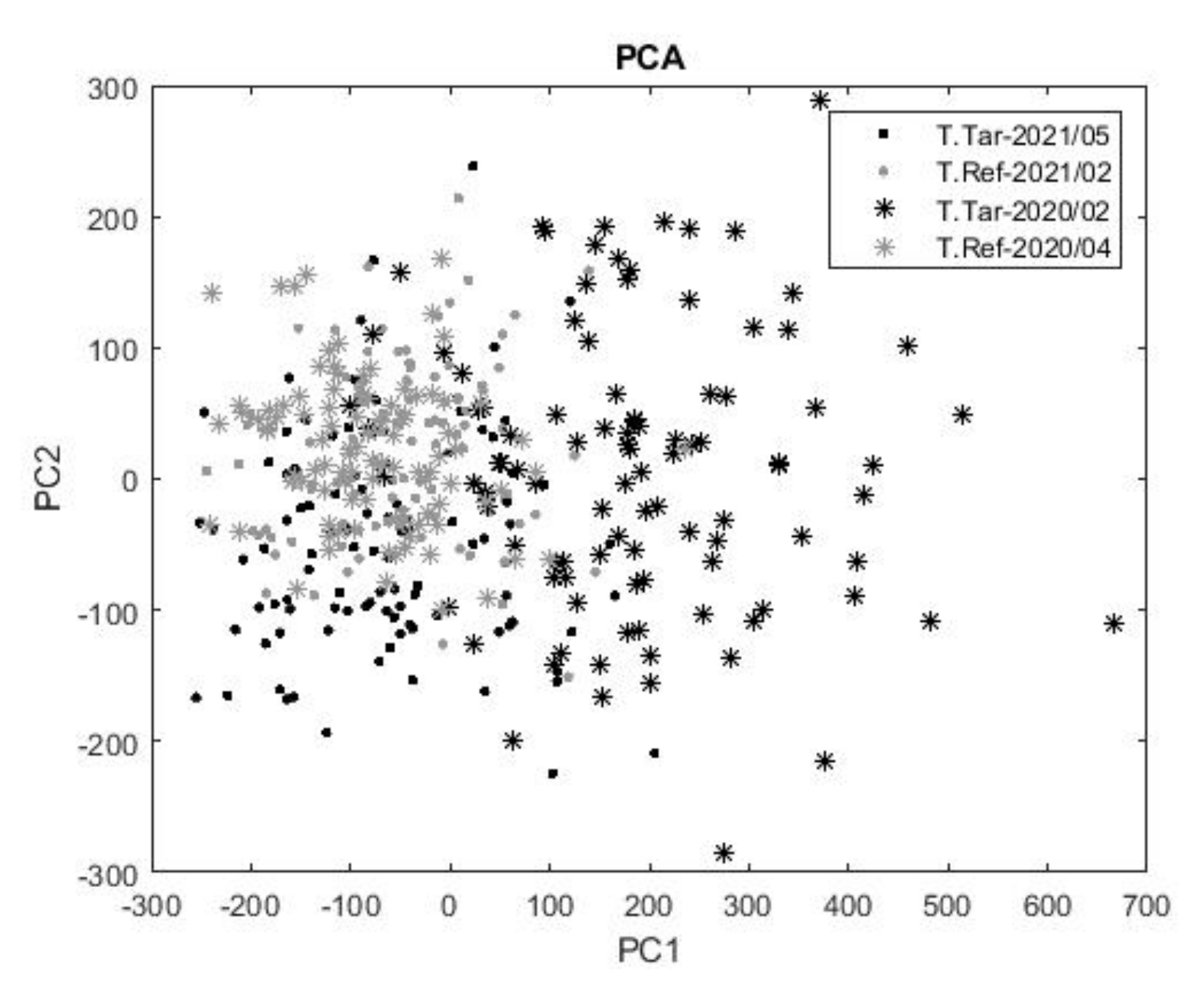
39]. In this framework then, a simple yet effective Novelty Metric based on PCA was used. The principal Principal Component Analysis was carried out on the whole pre-processed dataset. The result of the corresponding dimensional reduction is shown in
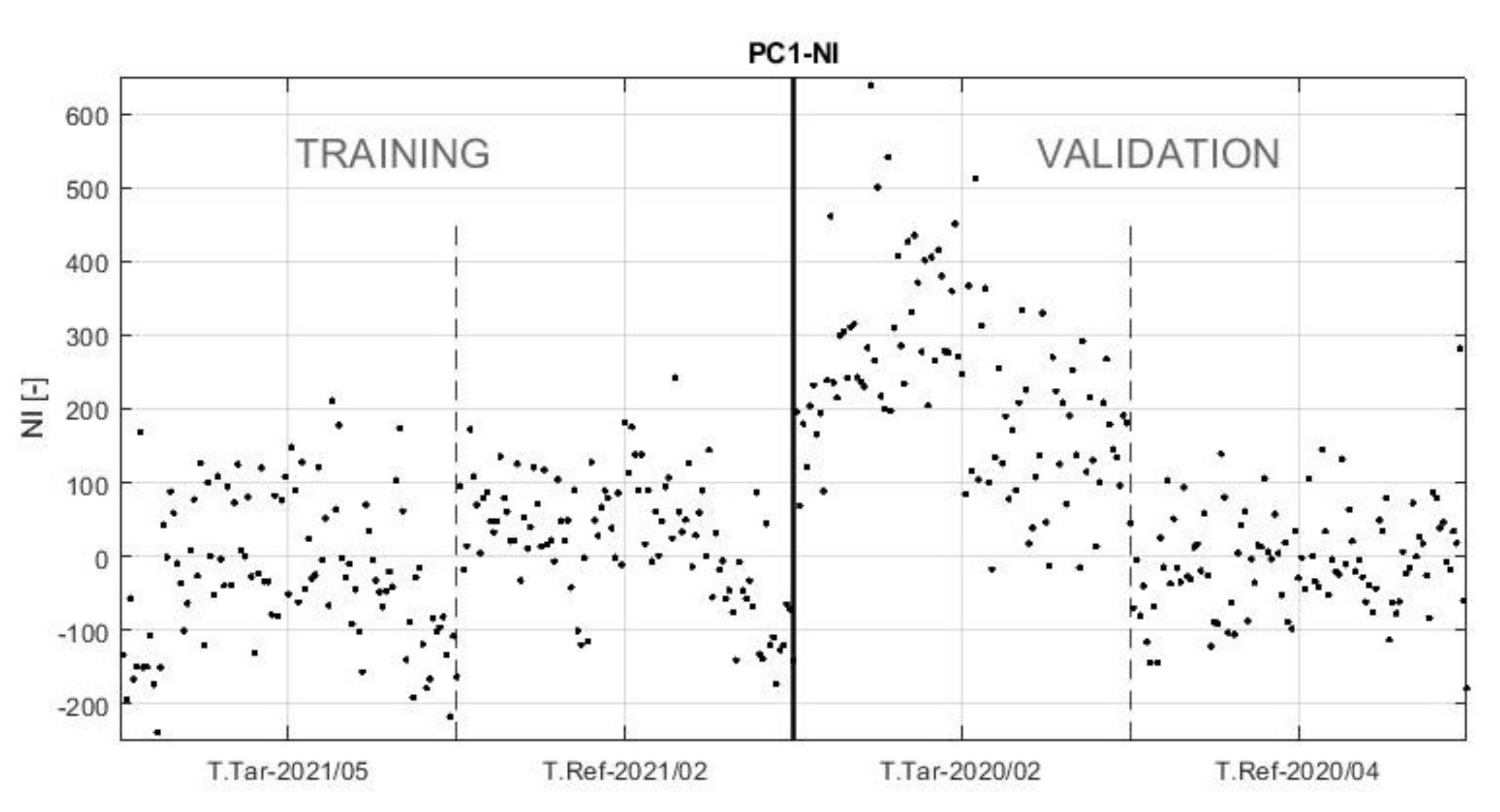
Figure 9. In this 2D representation only the first two principal directions are considered; nevertheless, these, respectively, explain 68% and 22% of the total variability in the dataset. As is clearly visible, along PC1 most of the variability is related to a shift of the turbine T.Tar cloud to higher values, further away with respect to the Training and Healthy Validation clouds. Hence, the PC1 information can be used as a good Novelty Indicator. This NI is shown in
Figure 10 where the training and the validation sets are reported. The rationale for showing this Figure is a qualitative assessment of the fact that the NI is in general higher in the faulty validation data set, despite the measurements having been recorded almost 7 months before the failure: from this Figure, one can argue that the TCM vibration data can clearly highlight the presence of Novelty related to an anomalous health condition.
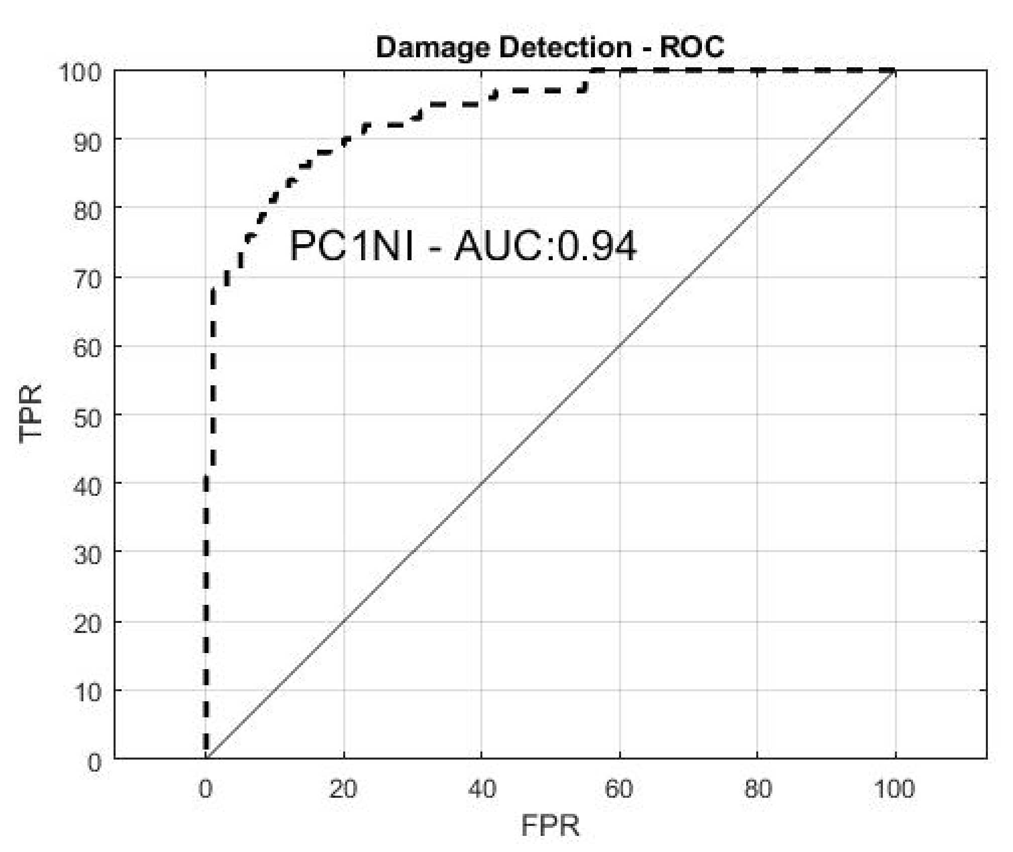
In order to complete the analysis, a quantitative result is helpful regarding the damage detection ability of such an NI indicator for the incipient damage on T.Tar: therefore, a Receiver Operating Characteristic (ROC) curve is reported in
Figure 11, in terms of true positive rate vs. false positive rate. The area under such a curve corresponds to 94% of the total, indicating a nearly optimal performance. In particular, if a false positive rate of 5% is accepted (i.e., the threshold set at NI = 158), more than 70% of the points coming from T.Tar in the faulty condition are correctly identified as damaged.
5. Conclusions
In the present work, a multi-scale approach for fault detection in wind turbine gearboxes was developed and tested on a real-world test case. The novelty of the work is due to the fact that the detection approaches are developed using the industrial data sets available from the standard SCADA and TCM systems. This is the main challenge faced in the present paper and the results unveil the pros and cons in using each kind of datum.
The early fault detection is possible using intuitive SCADA processing like the analysis of the
of the oil pressure before and after the gearbox filter. Even if this approach seems the most useful in the early fault diagnosis as the anomaly of the faulty machine has been clearly visible since the beginning (9 months before the turbine’s stop, see Figure
1), this kind of analysis is not useful to identify the faulty component.
A deeper diagnosis can be performed using the temperature measurements of the gearbox component recorded by the SCADA systems on a 10 min time scale. The raw trend of temperature is indeed not useful but the use of more complex modelling methods (like the SVR employed in this work) can unveil the abnormal positive drift of the error of model. The application of such an approach begins by establishing a baseline model using the dataset at the beginning of the period under investigation. When a fault in the gear is coming and producing heat, the actual temperature of the component is frequently higher than the temperature modelled by the SVR. In this way, temperature monitoring can be conducted, basing on the results of present work, a very powerful tool for early fault diagnosis as it allowed the discovery of the fault 5–6 months before the turbine’s stop (see
Figure 7b). Such a conclusion is different from what can be obtained using only raw temperature data that are usually considered only for late detection. The main limit of this approach is that a training period is always necessary so that, in our case, the first 3 months of data cannot be used to detect any anomaly. A joint analysis of
(Figure
1) for the oil filter and temperature error (
Figure 7) can only be synchronized using a larger dataset for temperature processing in order to create a trained reference model in the machine learning approach.
The approach used for TCM vibration data analysis confirms that the use of high resolution measurements is one of the best options for early detection and can give quite detailed information about the real location of the fault.
Anyway a critical issue in the interpretation of such results is that the precise location of the faulty component was not really discovered through the use of vibrations or SVR-temperature analysis. Both approaches clearly indicate a problem in the gear but the actual faulty component was the main bearing sustaining the main shaft at the interface with the gearbox.
This can be discussed as follows:
The individuation of the damage through temperature analysis is easier as the overheating increases and this can be very likely produced near the high speed components of the gear also if the damage is not exactly located there;
The detection of faults through vibration signals in the low speed components (such the main shaft) can be successful only when using sufficiently long time histories.
We can finally conclude that the tested approaches are really powerful to use in fault diagnosis but the drawback of using measurements coming from the industrial SCADA and TCM systems prevented from precisely locating the affected component.
Both approaches were able to indirectly detect the problem, because the misalignment of the main shaft was finally affecting also the operation of the gear.
Author Contributions
Conceptualization, F.C., A.P.D., F.N. and L.G.; data curation, F.C., A.P.D. and F.N.; formal analysis, F.C., A.P.D. and L.G.; investigation, F.C., A.P.D., F.N. and L.G.; methodology, F.C:, A.P.D. and L.G.; project administration, F.C. and L.G.; software, A.P.D. and F.N.; supervision, F.C. and L.G., validation, F.C., A.P.D., F.N. and L.G.; writing—original draft, F.N. and A.P.D.; writing—review and editing, F.C. and L.G. All authors have read and agreed to the published version of the manuscript.
Funding
This research received no external funding.
Acknowledgments
The author thanks Ludovico Terzi and Andrea Lombardi from the company ENGIE Italia for technical support and for providing the data sets employed for the study.
Conflicts of Interest
The authors declare no conflict of interest.
References
- Amano, R.S. Review of wind turbine research in 21st century. J. Energy Resour. Technol. 2017, 139, 050801. [Google Scholar] [CrossRef]
- Abdelbaky, M.A.; Liu, X.; Jiang, D. Design and implementation of partial offline fuzzy model-predictive pitch controller for large-scale wind-turbines. Renew. Energy 2020, 145, 981–996. [Google Scholar] [CrossRef]
- Peeters, C.; Guillaume, P.; Helsen, J. Vibration-based bearing fault detection for operations and maintenance cost reduction in wind energy. Renew. Energy 2018, 116, 74–87. [Google Scholar] [CrossRef]
- Kumar, R.; Ismail, M.; Zhao, W.; Noori, M.; Yadav, A.R.; Chen, S.; Singh, V.; Altabey, W.A.; Silik, A.I.; Kumar, G.; et al. Damage detection of wind turbine system based on signal processing approach: A critical review. Clean Technol. Environ. Policy 2021, 23, 561–580. [Google Scholar] [CrossRef]
- Tchakoua, P.; Wamkeue, R.; Ouhrouche, M.; Slaoui-Hasnaoui, F.; Tameghe, T.A.; Ekemb, G. Wind turbine condition monitoring: State-of-the-art review, new trends, and future challenges. Energies 2014, 7, 2595–2630. [Google Scholar] [CrossRef] [Green Version]
- Gonzalez, E.; Stephen, B.; Infield, D.; Melero, J.J. Using high-frequency SCADA data for wind turbine performance monitoring: A sensitivity study. Renew. Energy 2019, 131, 841–853. [Google Scholar] [CrossRef] [Green Version]
- Dai, J.; Yang, X.; Hu, W.; Wen, L.; Tan, Y. Effect investigation of yaw on wind turbine performance based on SCADA data. Energy 2018, 149, 684–696. [Google Scholar] [CrossRef]
- Byrne, R.; Astolfi, D.; Castellani, F.; Hewitt, N.J. A Study of Wind Turbine Performance Decline with Age through Operation Data Analysis. Energies 2020, 13, 2086. [Google Scholar] [CrossRef] [Green Version]
- Zaher, A.; McArthur, S.; Infield, D.; Patel, Y. Online wind turbine fault detection through automated SCADA data analysis. Wind Energy Int. J. Prog. Appl. Wind Power Convers. Technol. 2009, 12, 574–593. [Google Scholar] [CrossRef]
- Qiu, Y.; Feng, Y.; Infield, D. Fault diagnosis of wind turbine with SCADA alarms based multidimensional information processing method. Renew. Energy 2020, 145, 1923–1931. [Google Scholar] [CrossRef]
- Vidal, Y.; Pozo, F.; Tutivén, C. Wind turbine multi-fault detection and classification based on SCADA data. Energies 2018, 11, 3018. [Google Scholar] [CrossRef] [Green Version]
- Astolfi, D.; Castellani, F.; Terzi, L. Fault prevention and diagnosis through scada temperature data analysis of an onshore wind farm. Diagnostyka 2014, 15, 71–78. [Google Scholar]
- Astolfi, D.; Scappaticci, L.; Terzi, L. Fault diagnosis of wind turbine gearboxes through temperature and vibration data. Int. J. Renew. Energy Res. 2017, 7, 965–976. [Google Scholar]
- Barszcz, T.; Randall, R.B. Application of spectral kurtosis for detection of a tooth crack in the planetary gear of a wind turbine. Mech. Syst. Signal Process. 2009, 23, 1352–1365. [Google Scholar] [CrossRef]
- Maheswari, R.U.; Umamaheswari, R. Trends in non-stationary signal processing techniques applied to vibration analysis of wind turbine drive train—A contemporary survey. Mech. Syst. Signal Process. 2017, 85, 296–311. [Google Scholar] [CrossRef]
- Siegel, D.; Zhao, W.; Lapira, E.; AbuAli, M.; Lee, J. A comparative study on vibration-based condition monitoring algorithms for wind turbine drive trains. Wind Energy 2014, 17, 695–714. [Google Scholar] [CrossRef]
- Luo, H.; Hatch, C.; Kalb, M.; Hanna, J.; Weiss, A.; Sheng, S. Effective and accurate approaches for wind turbine gearbox condition monitoring. Wind Energy 2014, 17, 715–728. [Google Scholar] [CrossRef]
- Sawalhi, N.; Randall, R.B.; Forrester, D. Separation and enhancement of gear and bearing signals for the diagnosis of wind turbine transmission systems. Wind Energy 2014, 17, 729–743. [Google Scholar] [CrossRef]
- Sheldon, J.; Mott, G.; Lee, H.; Watson, M. Robust wind turbine gearbox fault detection. Wind Energy 2014, 17, 745–755. [Google Scholar] [CrossRef]
- Wang, J.; Gao, R.X.; Yan, R. Integration of EEMD and ICA for wind turbine gearbox diagnosis. Wind Energy 2014, 17, 757–773. [Google Scholar] [CrossRef]
- Xu, M.; Feng, G.; He, Q.; Gu, F.; Ball, A. Vibration characteristics of rolling element bearings with different radial clearances for condition monitoring of wind turbine. Appl. Sci. 2020, 10, 4731. [Google Scholar] [CrossRef]
- Elforjani, M.; Bechhoefer, E. Analysis of extremely modulated faulty wind turbine data using spectral kurtosis and signal intensity estimator. Renew. Energy 2018, 127, 258–268. [Google Scholar] [CrossRef]
- Elforjani, M. Diagnosis and prognosis of real world wind turbine gears. Renew. Energy 2020, 147, 1676–1693. [Google Scholar] [CrossRef]
- Elforjani, M.; Shanbr, S.; Bechhoefer, E. Detection of faulty high speed wind turbine bearing using signal intensity estimator technique. Wind Energy 2018, 21, 53–69. [Google Scholar] [CrossRef]
- Nilsson, K.; Ivanell, S.; Hansen, K.S.; Mikkelsen, R.; Sørensen, J.N.; Breton, S.P.; Henningson, D. Large-eddy simulations of the Lillgrund wind farm. Wind Energy 2015, 18, 449–467. [Google Scholar] [CrossRef]
- Papatheou, E.; Dervilis, N.; Maguire, A.E.; Antoniadou, I.; Worden, K. A performance monitoring approach for the novel Lillgrund offshore wind farm. IEEE Trans. Ind. Electron. 2015, 62, 6636–6644. [Google Scholar] [CrossRef] [Green Version]
- Sebastiani, A.; Castellani, F.; Crasto, G.; Segalini, A. Data analysis and simulation of the Lillgrund wind farm. Wind Energy 2021, 24, 634–648. [Google Scholar] [CrossRef]
- Antoniadou, I.; Manson, G.; Staszewski, W.; Barszcz, T.; Worden, K. A time-frequency analysis approach for condition monitoring of a wind turbine gearbox under varying load conditions. Mech. Syst. Signal Process. 2015, 64, 188–216. [Google Scholar] [CrossRef]
- Mauricio, A.; Qi, J.; Gryllias, K. Vibration-based condition monitoring of wind turbine gearboxes based on cyclostationary analysis. J. Eng. Gas Turbines Power 2019, 141. [Google Scholar] [CrossRef]
- Xin, G.; Hamzaoui, N.; Antoni, J. Extraction of second-order cyclostationary sources by matching instantaneous power spectrum with stochastic model—Application to wind turbine gearbox. Renew. Energy 2020, 147, 1739–1758. [Google Scholar] [CrossRef]
- Roshanmanesh, S.; Hayati, F.; Papaelias, M. Utilisation of Ensemble Empirical Mode Decomposition in Conjunction with Cyclostationary Technique for Wind Turbine Gearbox Fault Detection. Appl. Sci. 2020, 10, 3334. [Google Scholar] [CrossRef]
- Castellani, F.; Garibaldi, L.; Daga, A.P.; Astolfi, D.; Natili, F. Diagnosis of Faulty Wind Turbine Bearings Using Tower Vibration Measurements. Energies 2020, 13, 1474. [Google Scholar] [CrossRef] [Green Version]
- Mollasalehi, E.; Wood, D.; Sun, Q. Indicative fault diagnosis of wind turbine generator bearings using tower sound and vibration. Energies 2017, 10, 1853. [Google Scholar] [CrossRef] [Green Version]
- Turnbull, A.; Carroll, J.; McDonald, A. Combining SCADA and vibration data into a single anomaly detection model to predict wind turbine component failure. Wind Energy 2021, 24, 197–211. [Google Scholar] [CrossRef]
- Jiang, L.; Xiang, D.; Tan, Y.; Nie, Y.; Cao, H.; Wei, Y.; Zeng, D.; Shen, Y.; Shen, G. Analysis of wind turbine Gearbox’s environmental impact considering its reliability. J. Clean. Prod. 2018, 180, 846–857. [Google Scholar] [CrossRef]
- Vapnik, V. The Nature of Statistical Learning Theory; Springer Science & Business Media: Berlin, Germany, 2013. [Google Scholar]
- Liu, H.; Shah, S.; Jiang, W. On-line outlier detection and data cleaning. Comput. Chem. Eng. 2004, 28, 1635–1647. [Google Scholar] [CrossRef]
- MATLAB Help Center, Hampel. Available online: https://www.mathworks.com/help/signal/ref/hampel.html (accessed on 12 June 2021).
- Daga, A.P.; Fasana, A.; Garibaldi, L.; Marchesiello, S. Big Data management: A Vibration Monitoring point of view. In Proceedings of the 2020 IEEE International Workshop on Metrology for Industry 4.0 & IoT, Roma, Italy, 3–5 June 2020; pp. 548–553. [Google Scholar]
- Daga, A.P.; Garibaldi, L. Machine Vibration Monitoring for Diagnostics through Hypothesis Testing. Information 2019, 10, 204. [Google Scholar] [CrossRef] [Green Version]
- Astolfi, D.; Daga, A.; Natili, F.; Castellani, F.; Garibaldi, L. Wind turbine drive-train condition monitoring through tower vibrations measurement and processing. In Proceedings of the ISMA 2020—International Conference on Noise and Vibration Engineering, Virtual Conference, Online, 7–9 September 2020. [Google Scholar]
- Daga, A.P.; Fasana, A.; Marchesiello, S.; Garibaldi, L. The Politecnico di Torino rolling bearing test rig: Description and analysis of open access data. Mech. Syst. Signal Process. 2019, 120, 252–273. [Google Scholar] [CrossRef]
Figure 1.
Gearbox scheme. Figure adapted with permission from [
35]. Copyright 2018, Elsevier, publisher.
Figure 1.
Gearbox scheme. Figure adapted with permission from [
35]. Copyright 2018, Elsevier, publisher.
Figure 2.
Flow chart of SCADA data analysis: oil pressure and temperatures were studied in parallel to obtain a comprehensive overlook of the turbine’s conditions.
Figure 2.
Flow chart of SCADA data analysis: oil pressure and temperatures were studied in parallel to obtain a comprehensive overlook of the turbine’s conditions.
Figure 3.
Example of PCA dimension reduction: the principal components PC1 and PC2 are obtained as the mutually orthogonal directions where the variance of the original data is maximized, respectively, labelled as and .
Figure 3.
Example of PCA dimension reduction: the principal components PC1 and PC2 are obtained as the mutually orthogonal directions where the variance of the original data is maximized, respectively, labelled as and .
Figure 4.
Flow chart of TCM analysis: features extracted from high resolution vibration data were processed with PCA from which it resulted that PC1 and PC2 could be profitably used as discrimination parameters. In the end, a novelty index (NI) was defined to separate the dataset of healthy turbines from damaged ones.
Figure 5.
Evolution of oil filter pressure (in September 2020 the faulted turbine was stopped up to January 2021).
Figure 5.
Evolution of oil filter pressure (in September 2020 the faulted turbine was stopped up to January 2021).
Figure 6.
Gear bearing temperature trend.
Figure 6.
Gear bearing temperature trend.
Figure 7.
Gear bearing C temperature weekly average trend of raw data (a) and the error of the SVR model (b).
Figure 7.
Gear bearing C temperature weekly average trend of raw data (a) and the error of the SVR model (b).
Figure 8.
Main bearing temperature weekly average trend of raw data (a) and the error of the SVR model (b).
Figure 8.
Main bearing temperature weekly average trend of raw data (a) and the error of the SVR model (b).
Figure 9.
Plot of the PCA first and second principal components: as along the X axis of the plot the points of the faulty dataset appear separated from the healthy ones, PC1 was considered a valuable parameter for the detection of damage.
Figure 9.
Plot of the PCA first and second principal components: as along the X axis of the plot the points of the faulty dataset appear separated from the healthy ones, PC1 was considered a valuable parameter for the detection of damage.
Figure 10.
NI computed on the four considered datasets: the statistical difference between the Ref. validation dataset and the Tar. one is evidenced by the novelty index.
Figure 10.
NI computed on the four considered datasets: the statistical difference between the Ref. validation dataset and the Tar. one is evidenced by the novelty index.
Figure 11.
Evaluation of the performance of the TCM data analysis through the ROC curve, representing the False Positive Rate (FPR) vs. the True Positive Rate (TPR).
Figure 11.
Evaluation of the performance of the TCM data analysis through the ROC curve, representing the False Positive Rate (FPR) vs. the True Positive Rate (TPR).
Table 1.
Average values of in the period before the gearbox maintenance on T02 () and after (). Note that in general most of the turbines undergo a drop of pressure as a consequence of ordinary maintenance.
Table 1.
Average values of in the period before the gearbox maintenance on T02 () and after (). Note that in general most of the turbines undergo a drop of pressure as a consequence of ordinary maintenance.
| | Before (bar) | After (bar) |
|---|
| T01 | 0.22 | 0.13 |
| T02 | 0.71 | 0.07 |
| T03 | 0.10 | 0.14 |
| T04 | 0.28 | 0.18 |
| T05 | 0.22 | 0.06 |
| T06 | 0.21 | 0.16 |
| T07 | 0.19 | 0.10 |
| T08 | 0.36 | 0.07 |
| T09 | 0.05 | 0.03 |
| T10 | 0.33 | 0.09 |
Table 2.
Structure of the SVR regressions for the selected analysis.
Table 2.
Structure of the SVR regressions for the selected analysis.
Table 3.
Vibrational events considered for the analysis.
Table 3.
Vibrational events considered for the analysis.
| Id. Turbine | Period | Rot. Speed [RPM] | Power [kW] | Dataset |
|---|
| T.Tar | 2021/05 | 28 | 1999 | Training (Healty) |
| T.Ref | 2021/02 | 28.1 | 2003.8 | Training (Healty) |
| T.Tar | 2020/02 | 27.9 | 2005.9 | Validation (Faulty) |
| T.Ref | 2020/04 | 27.8 | 1887.9 | Validation (Healty) |
| Publisher’s Note: MDPI stays neutral with regard to jurisdictional claims in published maps and institutional affiliations. |
© 2021 by the authors. Licensee MDPI, Basel, Switzerland. This article is an open access article distributed under the terms and conditions of the Creative Commons Attribution (CC BY) license (https://creativecommons.org/licenses/by/4.0/).


