
A Novel Metric-Learning-Based Method for Multi-Instance Textureless Objects’ 6D Pose Estimation


Abstract
:1. Introduction
2. Methodology
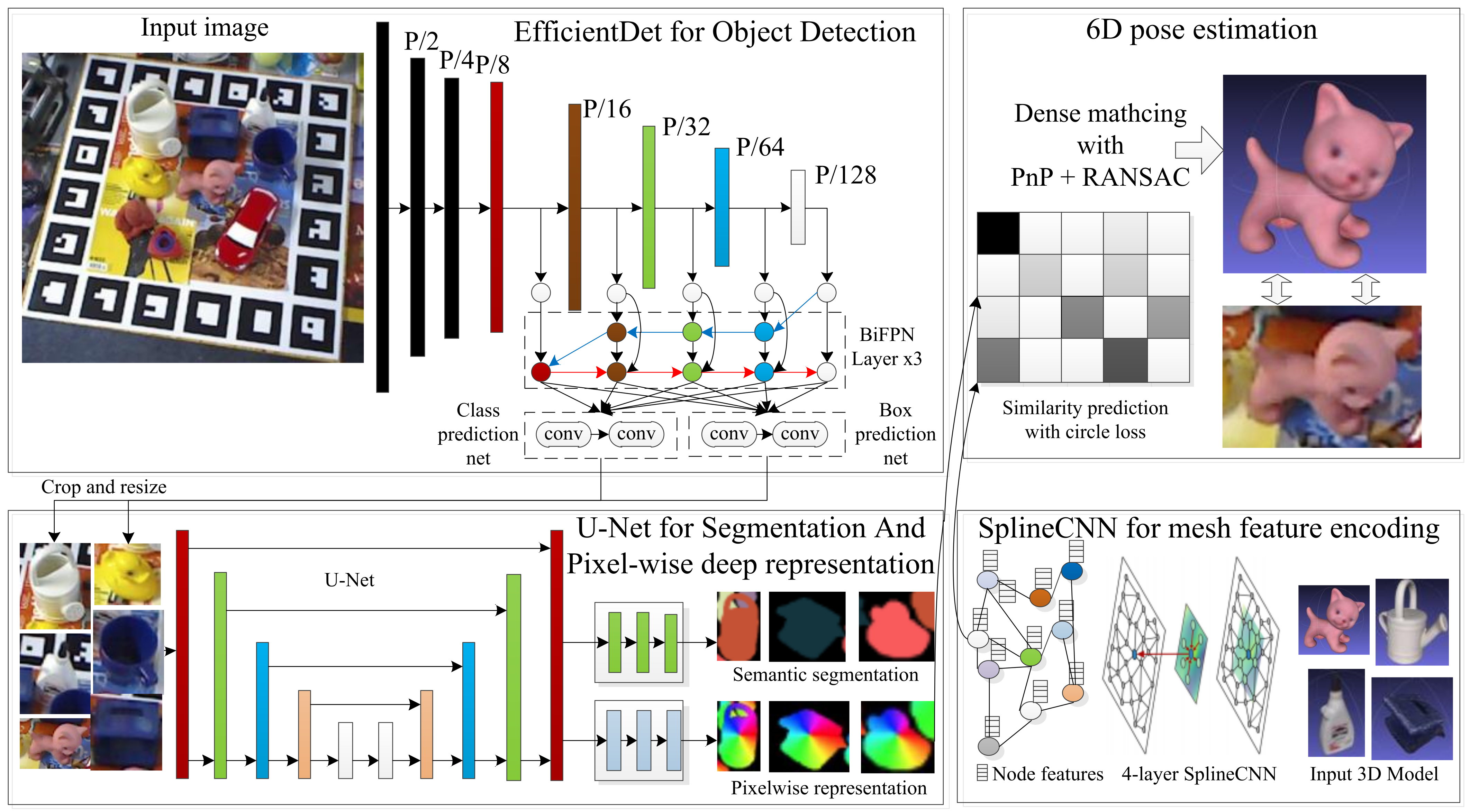
2.1. Overview
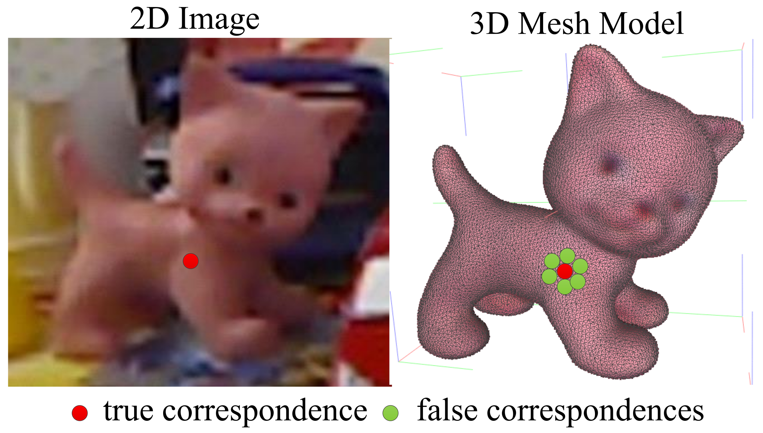
2.2. Masked Circle Loss for Matching Dense Correspondences
3. Results
3.1. Implementation Details
3.2. Evaluation Metric and Comparison
4. Conclusions and Future Work
Author Contributions
Funding
Data Availability Statement
Conflicts of Interest
References
- Choi, C.; Schwarting, W.; DelPreto, J.; Rus, D. Learning object grasping for soft robot hands. IEEE Robot. Autom. Lett. 2018, 3, 2370–2377. [Google Scholar] [CrossRef]
- Fang, H.S.; Wang, C.; Gou, M.; Lu, C. Graspnet-1billion: A large-scale benchmark for general object grasping. In Proceedings of the IEEE/CVF Conference on Computer Vision and Pattern Recognition, Seattle, WA, USA, 14–19 June 2020; pp. 11444–11453. [Google Scholar]
- Malik, A.A.; Andersen, M.V.; Bilberg, A. Advances in machine vision for flexible feeding of assembly parts. Procedia Manuf. 2019, 38, 1228–1235. [Google Scholar] [CrossRef]
- Yin, X.; Fan, X.; Zhu, W.; Liu, R. Synchronous AR Assembly Assistance and Monitoring System Based on Ego-Centric Vision. Assem. Autom. 2019, 39, 1–16. [Google Scholar] [CrossRef]
- Kleeberger, K.; Landgraf, C.; Huber, M.F. Large-scale 6d object pose estimation dataset for industrial bin-picking. In Proceedings of the 2019 IEEE/RSJ International Conference on Intelligent Robots and Systems (IROS), Macau, China, 4–8 November 2019; pp. 2573–2578. [Google Scholar]
- Mahler, J.; Goldberg, K. Learning deep policies for robot bin picking by simulating robust grasping sequences. In Proceedings of the Conference on Robot Learning, Mountain View, CA, USA, 13–15 November 2017; pp. 515–524. [Google Scholar]
- Ouyang, Z.; Sun, X.; Chen, J.; Yue, D.; Zhang, T. Multi-view stacking ensemble for power consumption anomaly detection in the context of industrial internet of things. IEEE Access 2018, 6, 9623–9631. [Google Scholar] [CrossRef]
- Zhang, H.; Cao, Q. Detect in RGB, optimize in edge: Accurate 6D pose estimation for texture-less industrial parts. In Proceedings of the 2019 International Conference on Robotics and Automation (ICRA), Montreal, QC, Canada, 20–24 May 2019; pp. 3486–3492. [Google Scholar]
- Peng, S.; Liu, Y.; Huang, Q.; Zhou, X.; Bao, H. Pvnet: Pixel-wise voting network for 6dof pose estimation. In Proceedings of the IEEE/CVF Conference on Computer Vision and Pattern Recognition (CVPR), Long Beach, CA, USA, 16–20 June 2019; pp. 4561–4570. [Google Scholar]
- Kehl, W.; Manhardt, F.; Tombari, F.; Ilic, S.; Navab, N. Ssd-6d: Making rgb-based 3d detection and 6d pose estimation great again. In Proceedings of the IEEE International Conference on Computer Vision (ICCV), Venice, Italy, 22–29 October 2017; pp. 1521–1529. [Google Scholar]
- Ke, Y.; Sukthankar, R. PCA-SIFT: A More Distinctive Representation for Local Image Descriptors. In Proceedings of the IEEE/CVF Conference on Computer Vision and Pattern Recognition (CVPR), Washington, DC, USA, 27 June–2 July 2004; pp. 506–513. [Google Scholar]
- Bay, H.; Ess, A.; Tuytelaars, T.; Van Gool, L. Speeded-up robust features (SURF). Comput. Vis. Image Underst. 2008, 110, 346–359. [Google Scholar] [CrossRef]
- Rublee, E.; Rabaud, V.; Konolige, K.; Bradski, G. ORB: An efficient alternative to SIFT or SURF. In Proceedings of the IEEE International Conference on Computer Vision (ICCV), Barcelona, Spain, 6–13 November 2011; pp. 2564–2571. [Google Scholar]
- He, Z.; Jiang, Z.; Zhao, X.; Zhang, S.; Wu, C. Sparse template-based 6-D pose estimation of metal parts using a monocular camera. IEEE Trans. Ind. Electron. 2019, 67, 390–401. [Google Scholar] [CrossRef]
- Chen, L.; Huang, P.; Cai, J. Extracting and Matching Lines of Low-Textured Region in Close-Range Navigation for Tethered Space Robot. IEEE Trans. Ind. Electron. 2018, 66, 7131–7140. [Google Scholar] [CrossRef]
- Tahri, O.; Chaumette, F. Complex objects pose estimation based on image moment invariants. In Proceedings of the IEEE International Conference on Robotics and Automation (ICRA), Barcelona, Spain, 18–22 April 2005; pp. 436–441. [Google Scholar]
- Meng, C.; Li, Z.; Sun, H.; Yuan, D.; Bai, X.; Zhou, F. Satellite pose estimation via single perspective circle and line. IEEE Trans. Aerosp. Electron. Syst. 2018, 54, 3084–3095. [Google Scholar] [CrossRef]
- Hinterstoisser, S.; Cagniart, C.; Ilic, S.; Sturm, P.; Navab, N.; Fua, P.; Lepetit, V. Gradient response maps for real-time detection of textureless objects. IEEE Trans. Pattern Anal. Mach. Intell. 2011, 34, 876–888. [Google Scholar] [CrossRef] [PubMed] [Green Version]
- Muñoz, E.; Konishi, Y.; Murino, V.; Del Bue, A. Fast 6D pose estimation for texture-less objects from a single RGB image. In Proceedings of the IEEE International Conference on Robotics and Automation (ICRA), Stockholm, Sweden, 16–21 May 2016; pp. 5623–5630. [Google Scholar]
- He, Z.; Wu, C.; Zhang, S.; Zhao, X. Moment-Based 2.5-D Visual Servoing for Textureless Planar Part Grasping. IEEE Trans. Ind. Electron. 2018, 66, 7821–7830. [Google Scholar] [CrossRef]
- Li, Y.; Wang, G.; Ji, X.; Xiang, Y.; Fox, D. Deepim: Deep iterative matching for 6d pose estimation. In Proceedings of the European Conference on Computer Vision (ECCV), Munich, Germany, 8–14 September 2018; pp. 683–698. [Google Scholar]
- Pavlakos, G.; Zhou, X.; Chan, A.; Derpanis, K.G.; Daniilidis, K. 6-dof object pose from semantic keypoints. In Proceedings of the IEEE International Conference on Robotics and Automation (ICRA), Singapore, 29 May–3 June 2017; pp. 2011–2018. [Google Scholar]
- Song, C.; Song, J.; Huang, Q. Hybridpose: 6d object pose estimation under hybrid representations. In Proceedings of the IEEE/CVF Conference on Computer Vision and Pattern Recognition (CVPR), Seattle, WA, USA, 16–18 June 2020; pp. 431–440. [Google Scholar]
- Labbé, Y.; Carpentier, J.; Aubry, M.; Sivic, J. Cosypose: Consistent multi-view multi-object 6d pose estimation. In European Conference on Computer Vision; Springer: Cham, Switzerland, 2020; pp. 574–591. [Google Scholar]
- Zakharov, S.; Shugurov, I.; Ilic, S. Dpod: 6d pose object detector and refiner. In Proceedings of the IEEE International Conference on Computer Vision (ICCV), Seoul, Korea, 27–28 October 2019; pp. 1941–1950. [Google Scholar]
- Wu, C.; Chen, L.; He, Z.; Jiang, J. Pseudo-Siamese Graph Matching Network for Textureless Objects’ 6D Pose Estimation. IEEE Trans. Ind. Electron. 2021, 1. [Google Scholar] [CrossRef]
- Lepetit, V.; Moreno-Noguer, F.; Fua, P. Epnp: An accurate o (n) solution to the pnp problem. Int. J. Comput. Vis. 2009, 81, 155. [Google Scholar] [CrossRef] [Green Version]
- Hinterstoisser, S.; Lepetit, V.; Ilic, S.; Holzer, S.; Bradski, G.; Konolige, K.; Navab, N. Model based training, detection and pose estimation of texture-less 3d objects in heavily cluttered scenes. In Proceedings of the Asian Conference on Computer Vision (ACCV), Daejeon, Korea, 5–9 November 2012; pp. 548–562. [Google Scholar]
- Brachmann, E.; Krull, A.; Michel, F.; Gumhold, S.; Shotton, J.; Rother, C. Learning 6D object pose estimation using 3D object coordinates. In Lecture Notes in Computer Science (Including subseries Lecture Notes in Artificial Intelligence and Lecture Notes in Bioinformatics); Springer: Cham, Switzerland, 2014. [Google Scholar] [CrossRef] [Green Version]
- Tan, M.; Pang, R.; Le, Q.V. Efficientdet: Scalable and efficient object detection. In Proceedings of the IEEE/CVF Conference on Computer Vision and Pattern Recognition, Seattle, WA, USA, 13–19 June 2020; pp. 10781–10790. [Google Scholar]
- Zhang, Z.; Sabuncu, M.R. Generalized cross entropy loss for training deep neural networks with noisy labels. In Proceedings of the 32nd Conference on Neural Information Processing Systems (NeurIPS), Montreal, QC, Canada, 3–8 December 2018. [Google Scholar]
- Xiang, Y.; Schmidt, T.; Narayanan, V.; Fox, D. PoseCNN: A Convolutional Neural Network for 6D Object Pose Estimation in Cluttered Scenes. In Proceedings of the Robotics: Science and Systems (RSS) XIV, Pittsburgh, PA, USA, 26–30 June 2018; pp. 129–136. [Google Scholar]
- Sun, Y.; Cheng, C.; Zhang, Y.; Zhang, C.; Zheng, L.; Wang, Z.; Wei, Y. Circle loss: A unified perspective of pair similarity optimization. In Proceedings of the IEEE/CVF Conference on Computer Vision and Pattern Recognition, Seattle, WA, USA, 13–19 June 2020; pp. 6398–6407. [Google Scholar]
- Hodaň, T.; Sundermeyer, M.; Drost, B.; Labbé, Y.; Brachmann, E.; Michel, F.; Rother, C.; Matas, J. BOP challenge 2020 on 6D object localization. In European Conference on Computer Vision; Springer: Cham, Switzerland, 2020; pp. 577–594. [Google Scholar]
- Paszke, A.; Gross, S.; Massa, F.; Lerer, A.; Bradbury, J.; Chanan, G.; Killeen, T.; Lin, Z.; Gimelshein, N.; Antiga, L.; et al. Pytorch: An imperative style, high-performance deep learning library. In Proceedings of the Advances in Neural Information Processing Systems, Vancouver, BC, Canada, 8–14 December 2019; pp. 8026–8037. [Google Scholar]
- Kingma, D.P.; Ba, J. Adam: A method for stochastic optimization. arXiv 2014, arXiv:1412.6980. [Google Scholar]
- Cignoni, P.; Callieri, M.; Corsini, M.; Dellepiane, M.; Ganovelli, F.; Ranzuglia, G. Meshlab: An open-source mesh processing tool. In Proceedings of the Eurographics Italian Chapter Conference, Salerno, Italy, 12–13 November 2008; Volume 2008, pp. 129–136. [Google Scholar]


| Methods | HybridPose | DPOD | PSGMN | Proposed Method |
|---|---|---|---|---|
| 89.3 | 86.2 | 93.9 | 96.5 | |
| 83.2 | 85.3 | 88.5 | 92.0 | |
| 76.5 | 77.6 | 81.0 | 87.3 | |
| 64.1 | 69.8 | 74.5 | 82.6 |
| Methods | HybridPose | DPOD | PSGMN | Proposed Method |
|---|---|---|---|---|
| 0.1-ADD | 72.2 | 71.4 | 76.5 | 84.3 |
| 0.08-ADD | 64.3 | 65.2 | 72.3 | 79.4 |
| 0.05-ADD | 51.1 | 53.3 | 57.9 | 74.7 |
Publisher’s Note: MDPI stays neutral with regard to jurisdictional claims in published maps and institutional affiliations. |
© 2021 by the authors. Licensee MDPI, Basel, Switzerland. This article is an open access article distributed under the terms and conditions of the Creative Commons Attribution (CC BY) license (https://creativecommons.org/licenses/by/4.0/).
Share and Cite
Wu, C.; Chen, L.; Wu, S. A Novel Metric-Learning-Based Method for Multi-Instance Textureless Objects’ 6D Pose Estimation. Appl. Sci. 2021, 11, 10531. https://doi.org/10.3390/app112210531
Wu C, Chen L, Wu S. A Novel Metric-Learning-Based Method for Multi-Instance Textureless Objects’ 6D Pose Estimation. Applied Sciences. 2021; 11(22):10531. https://doi.org/10.3390/app112210531
Chicago/Turabian StyleWu, Chenrui, Long Chen, and Shiqing Wu. 2021. "A Novel Metric-Learning-Based Method for Multi-Instance Textureless Objects’ 6D Pose Estimation" Applied Sciences 11, no. 22: 10531. https://doi.org/10.3390/app112210531