Article

A Switched Approach to Image-Based Stabilization for Nonholonomic Mobile Robots with Field-of-View Constraints

Department of Robotics Engineering, University of Shanghai for Science and Technology, Shanghai 200093, China
Appl. Sci. 2021, 11(22), 10895; https://doi.org/10.3390/app112210895
Submission received: 23 October 2021 / Revised: 14 November 2021 / Accepted: 15 November 2021 / Published: 18 November 2021

Abstract

:
This paper presents a switched visual servoing strategy for maneuvering the nonholonomic mobile robot to the desired configuration while keeping the tracked image points in the vision of the camera. Firstly, a pure backward motion and a pure rotational motion are applied to the mobile robot in succession. Thus, the principle point and the scaled focal length in x direction of the camera are identified through the visual feedback from a fixed onboard camera. Secondly, the identified parameters are used to build the system model in polar-coordinate representation. Then an adaptive non-smooth controller is designed to maneuver the mobile robot to the desired configuration under the nonholonomic constraint. And a switched strategy which consists of two image-based controllers is utilized for keeping the features in the field-of-view. Simulation results are presented to validate the effectiveness of the proposed approach.

1. Introduction

External visual sensors are more effective for the closed-loop control of nonholonomic mobile robots than the dead reckoning of internal sensors which can not achieve precise mobile robot poses because of slippage [1,2,3,4]. Visual servoing directly uses the visual information from the onboard camera to design the controller or to estimate the pose of the mobile robot. Existing works on visual servoing of wheeled mobile robots can be mainly formulated as tracking moving objects [5,6,7], tracking given path [8,9,10] and regulating toward a set-point [11,12,13]. Due to the peculiar nature of nonholonomic mobile robots, the set-point stabilization control of the mobile robot is more challenging than tracking problems. This paper deals with the stabilization problem of a nonholonomic mobile robot equipped with a fixed onboard pinhole camera that has a limited field-of-view.
According to Brockett’s necessary condition [14], mobile robots can not be stabilized via smooth time-invariant static feedback control which makes the existing manipulator visual servo controllers fail in mobile robots. Thus new nonlinear strategies have been developed, such as discontinuous controllers [15] and time-varying controllers [16]. Mariottini et al. [11] exploit the epipolar geometry to build the system model and zero the epipoles to align the robot with the goal in a straight line by using an input-output linearizing feedback control law. Then a proportional control law can decrease the translation error in the last stage. Fang et al. [12] utilize the 2D and 3D hybrid method to design a time-varying controller which introduces a sinusoidal function to rebuild the system state. Zhang et al. [13] also decompose the homography matrix to get the system states which are used in discontinuous change of coordinates to cope with the nonholonomic constraints of the mobile robot. Furthermore, a pan-tilt camera is used to deal with the vision constraint. All above control strategies do not need any priori 3D knowledge of the scene. However, the camera intrinsic parameters should be precisely calibrated in advance.
Consider the mobile robots with an uncalibrated camera, some robust visual servo strategies and self-calibration methods have been reported in [17,18,19,20,21]. López-Nicolás et al. [17] develop the control laws for three class optimal paths by using the entries in the homography matrix, while the optimal paths are generated under both the nonholonomic constraints and the field-of-view constraints [22]. Huang et al. [18] directly use the elements of the homography matrix building the error model, while two linear extended state observers are designed to compensate for the parameter uncertainties arising from the unknown 3D information and intrinsic parameters. Li et al. [19] propose a three-stage strategy including a rotation pointing to the goal, a straight line movement toward the goal, and a rotation regulating the desired pose. The intrinsic parameters estimated in the first stage are used in the latter two stages. Besides, Fang et al. [20] provide a geometric method for calibration of the camera principle point which uses the theorem that the parallel lines along the camera optical axis will meet in the principle point. This method is robust to radical distortion and the variation of the focal length. De Luca et al. [21] design a depth observer to estimate the depth online for regulating the mobile manipulator to desired configuration. This method can be extended to estimate the focal length of the camera.
Most visual servoing strategies for nonholonomic mobile robots assume the target remaining in the field-of-view during the regulation process. However, as the limited field-of-view of the pinhole camera, the vision constraint is an ineluctable problem of the mobile robot regulation. Chesi et al. [23] construct a switched approach consists of position-based rotational and translational control laws, and a backward motion for the manipulator, while the strategy is hard to extend to the mobile robot for the nonholonomic constraints. Murrieri et al. [24] present a hybrid-control approach deduced from five different Lyapunov functions with a polar coordinate presentation. The switching conditions are decided by 3D information of the feature points. Gans et al. [25] prove the controllability and stability of the control scheme for the optimal path in [22]. However, Salaris et al. demonstrate the optimal path in [22] is valid locally, which means the initial position should be close to the goal. So a complete synthesis for the whole plane of the motion is presented to extend the region of the initial point [26]. Then the vision constraints are considered not only in the horizontal directions but also in the vertical directions [27], and the ε -optimal paths start from each point in the motion region are provided. Ma et al. [28] design a shortest path between the initial pose and desired pose by using a pan-tilt camera to increase the horizontal field-of-view and vertical field-of-view. Karimian and Tron [29] apply two control fields being tangent and normal to ellipsoids to solve the problem of navigation, where the normal field is utilized to adjust the distance between the mobile robot and landmarks to satisfy the field-of-view constraints. All above motion planning research work on the base path generated by a position-based strategy.
In this paper, a switched image-based visual servoing strategy is proposed for the nonholonomic mobile robots equipped with a limited field-of-view camera. Specifically, a pure backward motion is imposed on the mobile robot to get the principal point of the camera. Next, a pure rotational motion is applied to the robot to identify the scaled focal length in the x direction. Then the identified camera intrinsic parameters are used to structure the image features in a polar coordinate presentation which is similar to the 3D pose of the mobile robot in the polar coordinate. Subsequently, an adaptive non-smooth controller is designed under nonholonomic constraints. A switched strategy is designed for keeping the features in the field-of-view, which consists of two image-based control laws. Simulation results are given to show the practicality of the proposed approach. This work has no need for precise calibration of the camera in advance. The main contribution is that two image-based control laws are used to keep the features in view during the regulation of the mobile robot under nonholonomic constraints. During the regulation task, only the visual information from a fixed pinhole camera can be used which makes the proposed approach more practical.
The remainder of the paper is organized as follows. Section 2 formulates the visual stabilization problem with vision constraint in detail. Section 3 identifies the camera principle point and the scaled focal length in x direction step-by-step. Then the estimated parameters are used to build the system model in polar-coordinate. An adaptive non-smooth controller combined with a switched strategy are designed in Section 4. Simulation results in Section 5 shows the effectiveness of this approach.

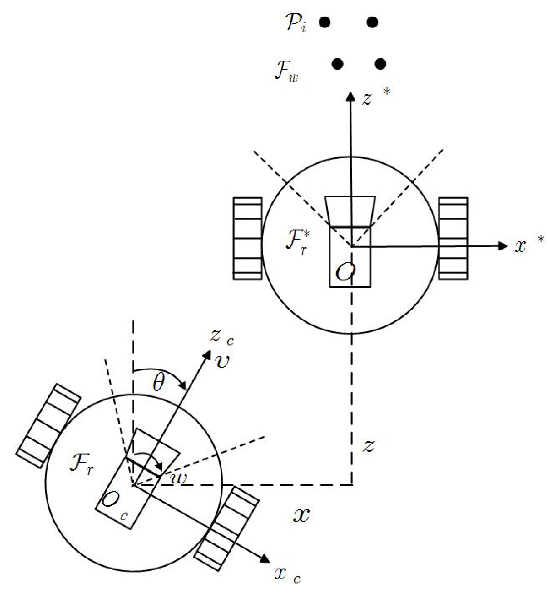
2. Problem Formulation

The mobile robot with a limited field-of-view camera system and the coordinates are described in Figure 1. The frame F c of the fixed onboard camera is consistent with the robot frame F r . So the camera is regarded as a part of the mobile robot. Consider a fixed frame F w which is consistent with the robot frame F r * when the mobile robot is in the desired configuration. A right-handed frame is defined with origin O and x axis is parallel to the robot wheel axis, z axis is along the camera optical axis, y axis is orthogonal to the motion plane, respectively. The posture state of the mobile robot is described by X ( t ) = ( x ( t ) , z ( t ) , θ ( t ) ) T , where ( x ( t ) , z ( t ) ) are the position coordinates of the mobile robot in the Cartesian plane, and θ ( t ) is the orientation of the mobile robot with respect to z axis as shown in Figure 1. The kinematics of the mobile robot can be expressed as
x ˙ = v sin θ z ˙ = v cos θ θ ˙ = w ,
where v , w are the linear and angular velocities that are used as the control inputs of the mobile robot.
P i R 3 , i = 1 , 2 , 3 , 4 are the static points in the world frame F w . In order to focus on the proposed method and simplify the system modeling, four marker points are used in this work while at least two points have the same height in the y axis direction but not in the camera optical axis plane to avoid the singular structure. In the actual scenario application, the extraction and matching of image points could be carried out using SIFT, SURF and ORB features instead of the marker points. Then the perspective projection geometry for point P i is derived,
s i ( t ) 1 = 1 Z c i K 0 3 × 1 R T R T t r 0 1 × 3 1 P i 1 ,
where s i ( t ) = ( u i , v i ) , i = 1 , 2 , 3 , 4 are the image coordinates. Z c i is the depth of the point P i in the frame F c . R and t r defined as
R = c θ 0 s θ 0 1 0 s θ 0 c θ , t r = ( x , 0 , z ) T
are the rotation matrix and translation vector of the mobile robot with respect to the world frame, respectively. s θ and c θ are the abbreviations of sin θ and cos θ , respectively. The camera intrinsic matrix K is
K = f u 0 u 0 0 f v v 0 0 0 1 ,
where f u and f v are the scaled focal length in x and y directions, respectively. ( u 0 , v 0 ) are the coordinates of the principle point in pixels. Calculating the derivative of the image point in equation (2) with respect to time yields
s ˙ i ( t ) = u i u 0 Z c i f u ( u i u 0 ) 2 f u v i v 0 Z c i ( u i u 0 ) ( v i v 0 ) f u J ( s i , Z c i ) v w ,
where J ( s i , Z c i ) is the interaction matrix of an image point.
The desired image is taken at the desired configuration X * = ( 0 , 0 , 0 ) T m in advance. The desired image is used to guide the mobile robot from the current configuration to the desired configuration.

3. Self-Calibration of Camera Intrinsic Parameters

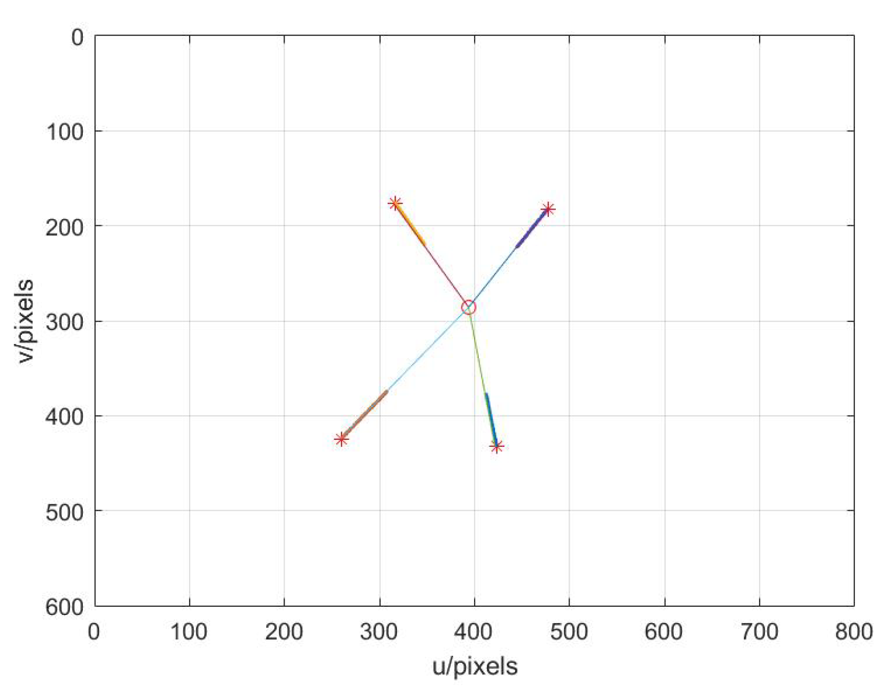
3.1. Self-Calibration of the Principle Point

According to the Theorem proposed [20], the image paths of the static feature points will meet in the principle point when the camera moves along the optical axis. To avoid the feature points escaping from the camera view, a pure backward motion is applied to the mobile robot. Four feature points are used so that four straight lines are calculated as
L i : a j u i + b j v i + c j = 0 , j = 1 , 2 , 3 , 4 .
Since all the straight lines pass through the principle point, the principle point ( u 0 , v 0 ) can be calculated through
L 0 : a j u 0 + b j v 0 + c j = 0 , j = 1 , 2 , 3 , 4 .
Then the lines and the principal point can be obtained by solving the following geometric distance step by step:
( a j , b j , c j ) = arg min i = 1 m a j u i + b i v i + c j 2
and
( u 0 , v 0 ) = arg min j = 1 4 a j u 0 + b j v 0 + c j 2 .
To solve problems (7) and (8), we use CVX which is a package for specifying and solving convex programs [30]. The result is ( u ^ 0 , v ^ 0 ) = ( 393.6890 , 285.9458 ) / p i x e l s shown in Figure 2.

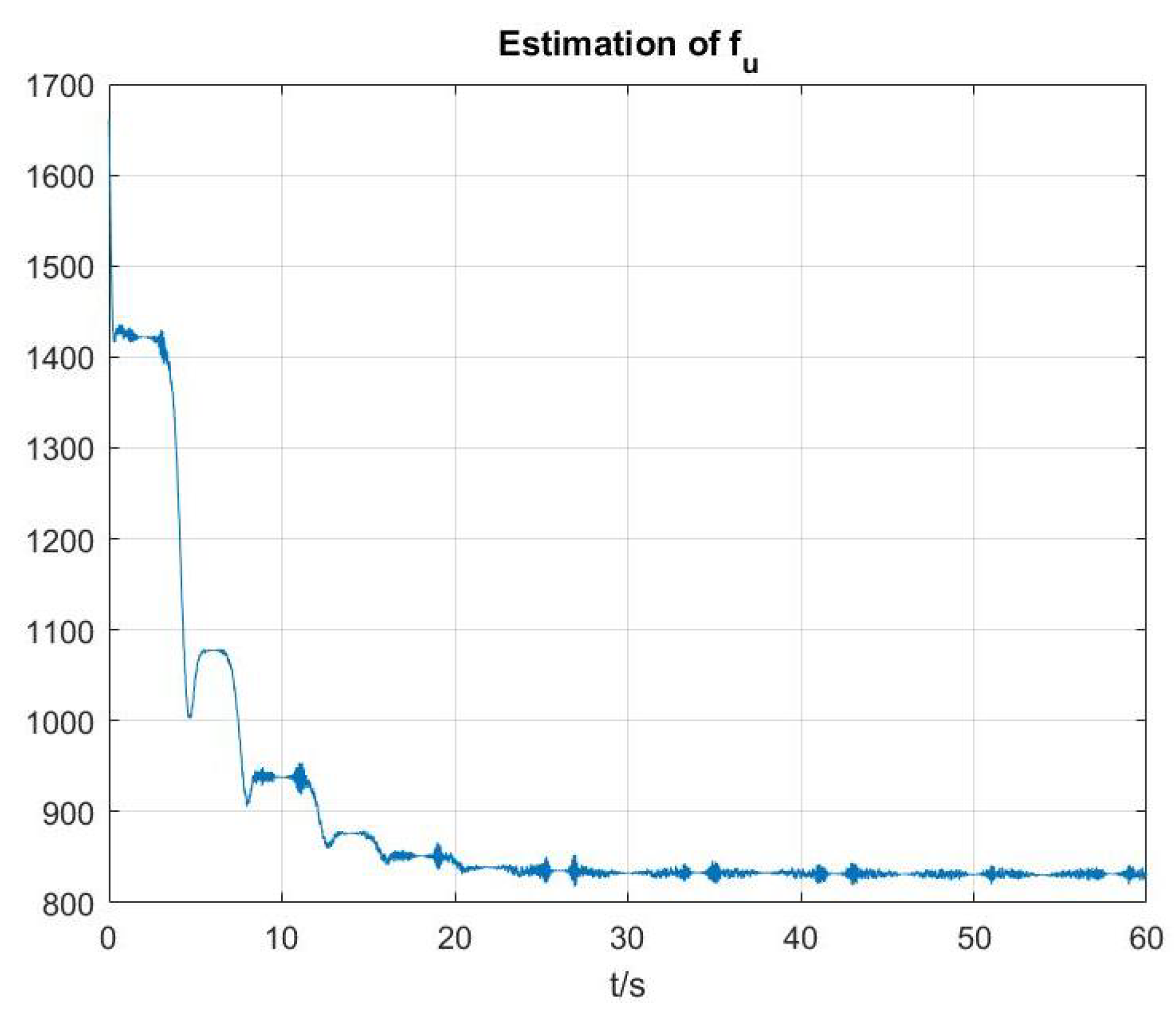
3.2. Self-Calibration of the Scaled Focal Length in x Direction

As the interaction matrix in (4) shows, pure rotation of the mobile robot do not depend on the depth but depends on the scaled focal length in x direction. Therefore, an focal length observer designed in [21] is exploited to the camera installed on the mobile robot. Let ξ = ( u ¯ , v ¯ , f u , 1 f u ) be the state vector, where u ¯ = u u 0 , v ¯ = v v 0 are the partially normalized image feature. Assume a pure rotational motion is applied to the mobile robot, the dynamic equations are expressed as
ξ ˙ = ( ξ 3 + ξ 1 2 ξ 4 ) ξ 1 ξ 2 ξ 4 0 0 w , y = ξ 1 ξ 2 .
Let ξ ^ R 4 be the estimation of the state ξ . By defining e = ξ ξ ^ as the estimate error vector, the nonlinear observer is designed as
ξ ^ ˙ = ( ξ ^ 3 + y 1 2 ξ ^ 4 ) y 1 y 2 ξ ^ 4 0 0 w + k 1 e 1 k 2 e 2 k 3 w e 1 k 4 ( y 1 2 w e 1 + y 1 y 2 w e 2 )
with k 1 , k 2 , k 3 , k 4 R + are positive parameters. Then we obtain the error dynamics
e ˙ = k 1 0 w y 1 2 w 0 k 2 0 y 1 y 2 w k 3 w 0 0 0 k 4 y 1 2 w k 4 y 1 y 2 w 0 0 H e .
Since a pure rotational motion is imposed on the mobile robot, it ensures w 2 0 , y 1 2 y 2 2 w 2 0 . The matrix H is a Hurwitz matrix. Thus the exponential convergence of the error system can be guaranteed. The partially normalized image features are obtained by applying the estimated principle point from the previous subsection, which are used in the observer (10). Then the result is f ^ u = 830.5416 /pixels and the evolution is shown in Figure 3.

4. Image-Based Visual Servoing with Limited Field-of-View

4.1. System Model Development

After self-calibration of the camera parameters, a new state variable [ η 1 , η 2 ] T is defined as
η 1 = u ¯ v ¯ , η 2 = f u 1 v ¯
to replace the states of (4). Correspondingly, the new desired state variables are defined as
η 1 * = u ¯ * v ¯ * , η 2 * = f u 1 v ¯ * .
Taking the time derivative of the new state variables and utilizing (4), the kinematics model is obtained as
η ˙ 1 = η 2 w η ˙ 2 = η 2 Z c i v + η 1 w = f u f v Y c i v + η 1 w .
Suppose the two points P i and P j have the same height in the y axis direction, i.e., Y c i = Y c j h > 0 , the relationship between the current camera configuration and desired configuration can be deduced through the two points as
P i c P j c = R T P i d P j d
with P c = R T ( P d t r ) where P c , P d denote the points in coordinate of the current camera configuration and the desired camera configuration, respectively. R and t r are the rotation matrix and translation vector defined in (3). It is clear that the new state variables have similar geometrical relations with the static points P . The quantities defined in the image plane η 1 i j = u ¯ i v ¯ i u ¯ j v ¯ j , η 2 i j = f u 1 v ¯ i f u 1 v ¯ j have the following relation as
η 1 i j η 2 i j = c θ s θ s θ c θ η 1 i j * η 2 i j * .
Then the angle θ is recovered by the following equation: sin θ = ( η 1 i j * η 2 i j η 2 i j * η 1 i j ) / ( η 1 i j * 2 + η 2 i j * 2 ) . Therefore, the objective of the visual stabilization task becomes the construction of appropriate velocities v , w to ensure that
η 1 η 1 * , η 2 η 2 * , θ 0 .
In order to facilitate the subsequent controller design, the error signals are defined as follows
e 1 e 2 = c θ s θ s θ c θ η 1 η 2 η 1 * η 2 *
and
e 0 = θ .
Considering the time derivative of the error signals and substituting (13) into them, the error system is obtained
e ˙ 0 = w e ˙ 1 = c v s θ e ˙ 2 = c v c θ ,
where c f u f v h > 0 is utilized to simplify the expression of (19).
The error system (19) has the similar formulations with the mobile robot kinematics model (1). To overcome the effects of the nonholonomic constraints on the mobile robot visual servoing system, a σ -process is applied to break the one-to-one correspondence of the system. The discontinuous coordinates transformation used [13,31] is introduced as follows
ρ = e 1 2 + e 2 2 α = a t a n e 1 e 2 e 0 ϕ = a t a n e 1 e 2
for building the system model. The new states in polar coordinates define a diffeomorphism in the region ρ 0 . Then taking the time derivative of these new states, the open-loop system model is developed as
ρ ˙ = s i g n ( e 2 ) c v cos α α ˙ = s i g n ( e 2 ) c ρ v sin α w ϕ ˙ = s i g n ( e 2 ) c ρ v sin α .
From the open-loop system (21), it is clear that a singularity problem happens when the state ρ vanishes. To deal with this situation, the control inputs in system (21) are designed to first maneuver the system to a small neighborhood of the desired value which means the mobile robot is close enough to the desired configuration. Then a proportional rotation is utilized to control the angle θ to zero. Thus the control objective turn to
lim t ρ ( t ) = 0 , lim t α ( t ) = 0 , lim t ϕ ( t ) = 0 .

4.2. Control Design without Constraints

According to (17) and (18), the system states in polar coordinate can be obtained directly. There is an unknown constant c in the system (21), an adaptive controller is designed based on the Lyapunov Theory as following:
v = s i g n ( e 2 ) k c 1 ρ cos α ,
w = k c 2 α + c ^ k c 1 sin α cos α α α + k c 3 ϕ ,
with the adaptive law of c ^ designed as
c ^ ˙ = k a k c 1 sin α cos α α + k c 3 ϕ ,
where k c 1 , k c 2 , k c 3 , k a R + are positive control parameters. Then substituting the control inputs (23) and (24) to the open-loop system (21), the closed-loop system can be obtained as
ρ ˙ = c k c 1 ρ cos 2 α α ˙ = k c 2 α + c ˜ k c 1 sin α cos α c ^ k c 1 k c 3 ϕ sin α cos α α ϕ ˙ = c k c 1 sin α cos α ,
where c ˜ = c c ^ is the parameter estimation error. Note that there exists the limit law l i m α 0 sin α α = 1 , such that there is no singularity problem for the closed-loop system (26) and the control law (24).
Theorem 1.
The proposed control law (23) and (24) with the parameter adaptive law (25) can drive the system states ρ , α , ϕ to zero in the sense that
lim t ρ ( t ) = 0 , lim t α ( t ) = 0 , lim t ϕ ( t ) = 0 .
Proof of Theorem 1.
Choose a Lyapunov function candidate as follows
V = 1 2 ρ 2 + 1 2 α 2 + k c 3 ϕ 2 + 1 2 k a c ˜ 2 .
Taking the time derivative of the function V and then substituting the closed-loop system (26), we obtain
V ˙ = ρ ρ ˙ + α α ˙ + k c 3 ϕ ϕ ˙ 1 k a c ˜ c ^ ˙ = c k c 1 ρ 2 cos 2 α k c 2 α 2 + c ˜ k c 1 α sin α cos α c ^ k c 1 k c 3 ϕ sin α cos α + c k c 1 k c 3 ϕ sin α cos α c ˜ k c 1 sin α cos α ( α + k c 3 ϕ ) = c k c 1 ρ 2 cos 2 α k c 2 α 2 .
Since the constant parameter c > 0 , it is easy to deduce that
V ˙ 0 .
According to (27) and (29), it is easy to concluded that
ρ ( t ) , α ( t ) , ϕ ( t ) , c ˜ ( t ) L
and to find out the point in the invariant set M
( ρ = 0 , α = 0 ) M .
Substituting (31) back to the closed-loop system (26) and parameter adaptive law (25), it is concluded that
c ^ ϕ = 0 , c ^ ˙ = 0 .
From (30), we know that c ^ L . It is concluded that c ^ is a nonzero constant. Thus
ϕ = 0 .
According to above analysis, it is obvious that the invariant set M only consists of the equilibrium point being ( ρ = 0 , α = 0 , ϕ = 0 , c ^ = c o n s t a n t ) M . Based on LaSalle’s invariance principle [32], we can infer that the system states converge to the equilibrium point asymptotically. The Theorem 1 is proved. □
When the states of the closed-loop system converge to zero asymptotically, a singularity problem will happen. To deal with this problem that the state ρ go to zero, an intuitive method is to set the linear velocity v to zero when the state ρ is smaller than a threshold. The angular velocity is designed as a pure proportional controller w = k w θ , with k w being a positive control gain. This is scheduled as the last stage.

4.3. A Switched Approach
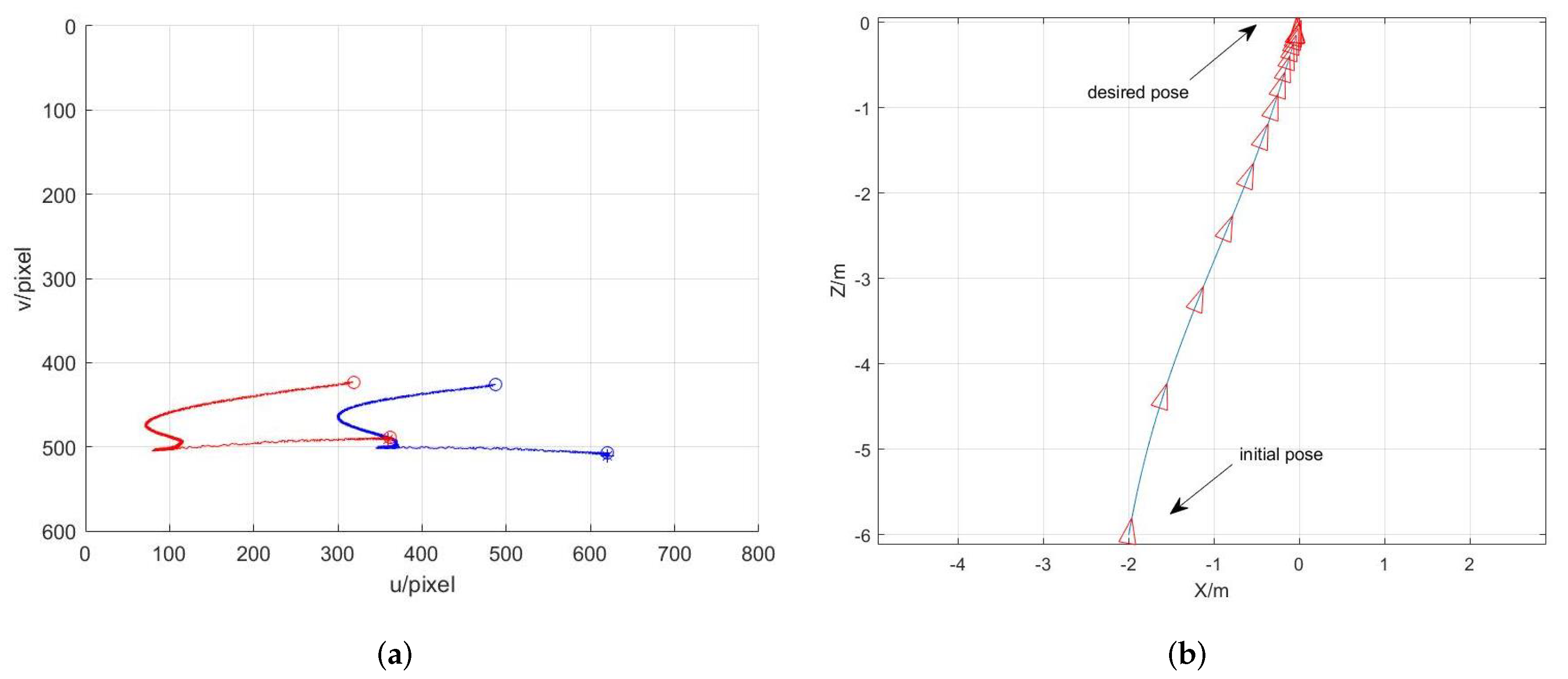
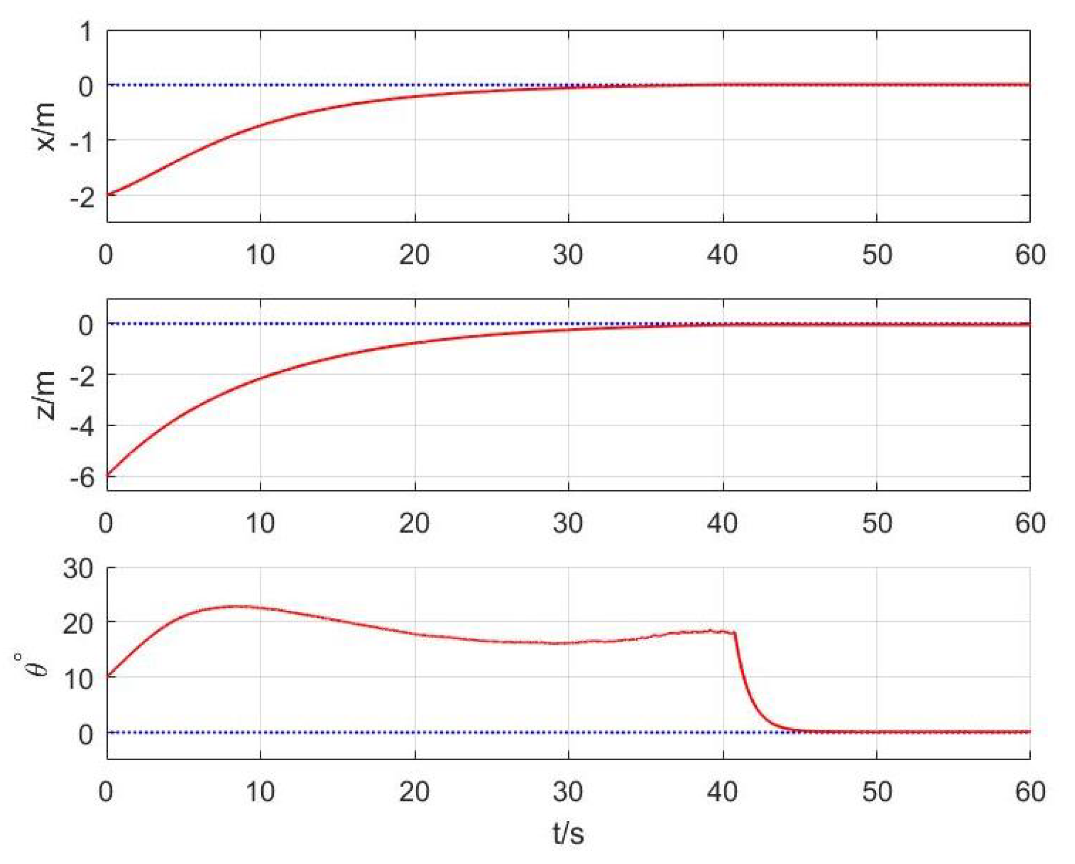
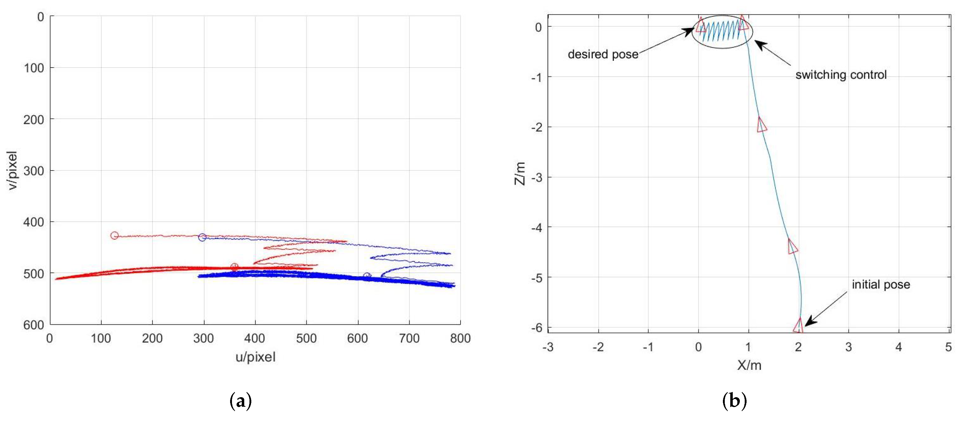
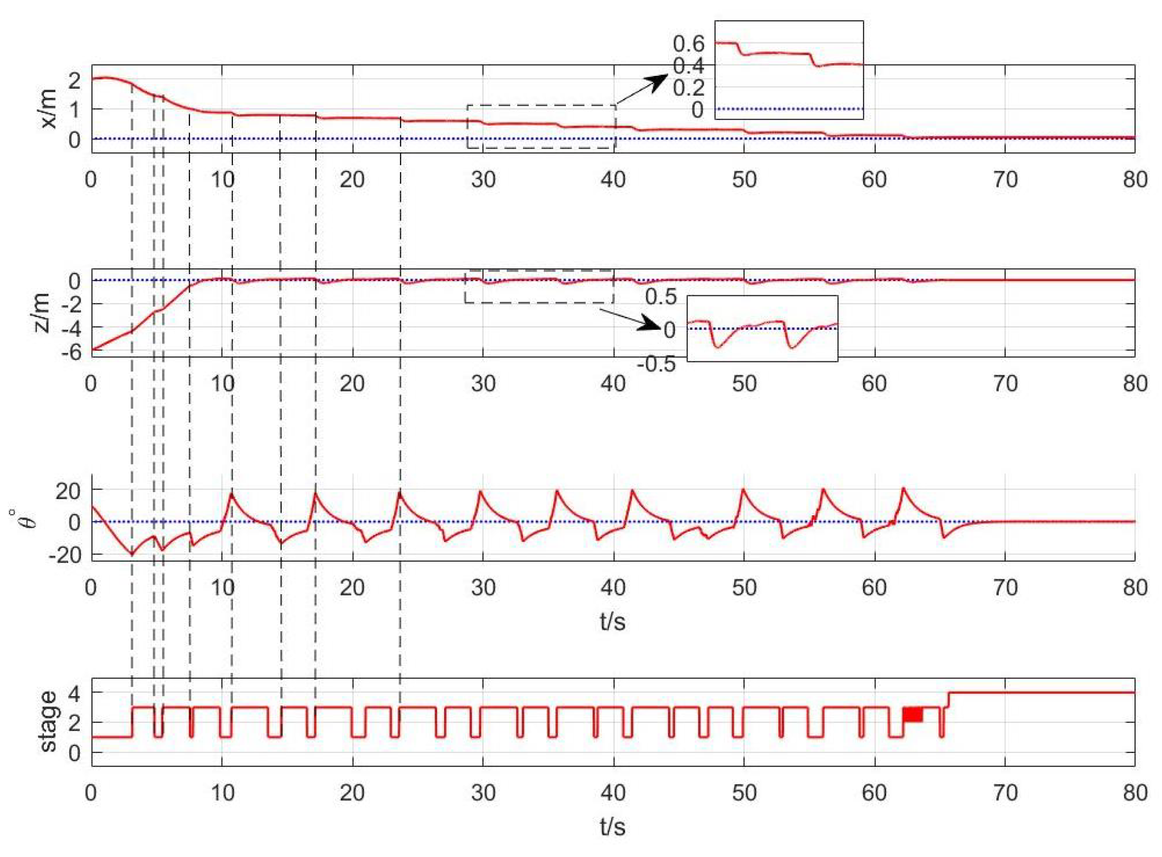
The controller designed in the previous subsection should work under an ideal situation that the feature points are always in the field-of-view. The system is built based on partial 3D information. It cannot be guaranteed that the visual features remain in the field-of-view during the stabilization task of the mobile robot. Thus an image-based switched approach is proposed to ensure the features remain in view.
Suppose that the motion of the robot is on a plane, the image points only escape the field-of-view from the left and right sides. A heuristic approach is to set two bounds at the left and right boundaries. If any feature point falls within the boundary, the control process switches to the image-based controllers which are designed as following
w = k t min ( u i ) min ( u i * ) v = k v v i v i v i *
and
w = k t max ( u i ) max ( u i * ) v = k v v i v i v i * ,
where v i is the coordinate in v direction of the corresponding image point with the min ( u i ) or max ( u i ) . k t , k v R + are positive control parameters. The control laws (34) are applied when an image point falls into the boundary area on the left. And the control laws (35) are applied when an image point falls into the boundary area on the right. The purpose of both sets of controllers is to bring the image points near the boundary back to the center of the field-of-view. In addition, a zone needs to be set in the center of the image to ensure that the controller can switch back to (23) and (24) when the image points fall into that zone. Together with this simple switching mechanism, it is guaranteed that the feature points could be kept in the field-of-view during the stabilization task of the mobile robot under the control of (23) and (24).

5. Simulations

Two sets of simulation results are presented to validate the proposed image-based switched approach for mobile robots. The Egt-toolbox [33] is used to accomplish the simulation. The virtual camera parameters are set as f u = 829.77 , f v = 826.59 , u 0 = 393.74 , v 0 = 285.87 . Two static points are selected as P 1 = [ 3 , 3 , 11 ] T m , P 2 = [ 0.5312 ] T m . The estimation error of the Principal point is less than 2.5 pixels, which is verified by multi-group experiments in [20]. Thus A random Gaussian noise with a deviation of 1.5 pixels, is added to the image points to verify the robustness.
The control parameters are shown in Table 1. These control parameters are utilized in the following two sets of simulations.
An initial pose of the mobile robot is selected as X 0 = [ 2 , 6 , 10 ] T . Simulation results are shown in Figure 4 and Figure 5. In Figure 4a, the trajectories of two image points pass through the circular points at the starting and ending positions, respectively. The star points represent the desired image points. The circular points at the end positions coincide with the star points, which indicates that the mobile robot has reached the desired configuration. This also can be seen from the motion trajectory of the mobile robot in Figure 4b. The state curves of the mobile robot are shown in Figure 5. At almost 41 seconds, the mobile robot was very close to the desired position, then a pure rotation control was applied to the robot. The threshold of the state ρ is set at 0.01 . In this case, no switching control occurs for the mobile robot. The feature points are always in the field-of-view during the stabilization task of the mobile robot, which is desirable. Next, a case that is not so ideal is considered.
In this case, an initial pose being X 0 = [ 2 , 6 , 10 ] T is selected. Simulations are shown in Figure 6 and Figure 7. As shown in Figure 6a, despite several round trips, the feature trajectories remain within the image boundaries. In Figure 7, the movement process of the mobile robot is divided into four stages. In stage 1, the control laws (23) and (24) are used. When an image feature falls into the left border area or the right border area of the image, it switches to stage 2 or stage 3 correspondingly. The controllers (34) and (35) are applied in stage 2 and stage 3, respectively. If the state ρ is smaller than the threshold, the last stage 4 is activated.
In this part, simulation results are provided to verify the effectiveness of the proposed strategy. According to above two sets of simulations, it is known that whether or not to start the switching process is related to the initial pose of the mobile robot. If the initial pose is good, the mobile robot can be driven to the desired pose quickly as shown in the first simulation. However, there is no basis for judging whether an initial pose is good or not good at present. This paper focus on the control strategy to keep two marker points in the field-of-view, which is a preliminary work. The efficiency of the control strategy is sacrificed to remain image features in view. Based on this work, the efficiency should be improved in the future work, which will be verified on a real mobile robot in an actual scenario.

6. Conclusions

A switching control approach with a polar coordinate based controller and two image-based controllers is proposed for the nonholonomic mobile robots. As the 3D angular information should be calculated for building the system model, the principle point and focal length in x direction of the camera are estimated by a self-calibration method in advance. A discontinuous coordinates transformation is applied to build the system model in polar coordinate. Then the asymptotical stability of the system is proven combined with a well designed adaptive controller. Afterward, two image-based controllers are designed to keep the features in the field-of-view during the visual stabilization task of the mobile robot. Simulation results demonstrate the proposed approach is effective. Although the image features could be kept in the field-of-view, the efficiency of the mobile robot is sacrificed with multiple round-trip movements. This will be considered in the future work.

Funding

This research received no external funding.

Conflicts of Interest

The authors declare no conflict of interests.

References

  1. Li, B.; Zhang, X.; Fang, Y.; Shi, W. Visual Servoing of Wheeled Mobile Robots without Desired Images. IEEE Trans. Cybern. 2019, 49, 2835–2844. [Google Scholar] [CrossRef] [PubMed]
  2. Li, B.; Zhang, X.; Fang, Y.; Shi, W. Visual Servo Regulation of Wheeled Mobile Robots with Simultaneous Depth Identification. IEEE Trans. Ind. Electron. 2018, 65, 460–469. [Google Scholar] [CrossRef]
  3. Ke, F.; Li, Z.; Yang, C. Robust Tube-Based Predictive Control for Visual Servoing of Constrained Differential-Drive Mobile Robots. IEEE Trans. Ind. Electron. 2018, 65, 3437–3446. [Google Scholar] [CrossRef]
  4. Wang, K.; Liu, Y.; Li, L. Visual Servoing Trajectory Tracking of Nonholonomic Mobile Robots Without Direct Position Measurement. IEEE Trans. Robot. 2014, 30, 1026–1035. [Google Scholar] [CrossRef]
  5. Freda, L.; Oriolo, G. Vision-based interception of a moving target with a nonholonomic mobile robot. Robot. Auton. Syst. 2007, 55, 419–432. [Google Scholar] [CrossRef]
  6. Tsai, C.Y.; Song, K.T.; Dutoit, X.; Brussel, H.V.; Nuttin, M. Robust visual tracking control system of a mobile robot based on a dual-Jacobian visual interaction model. Robot. Auton. Syst. 2009, 57, 652–664. [Google Scholar] [CrossRef]
  7. Chuang, H.M.; He, D.; Namiki, A. Autonomous Target Tracking of UAV Using High-Speed Visual Feedback. Appl. Sci. 2019, 9, 4552. [Google Scholar] [CrossRef] [Green Version]
  8. Zhang, K.; Chen, J.; Li, Y.; Gao, Y. Unified Visual Servoing Tracking and Regulation of Wheeled Mobile Robots with an Uncalibrated Camera. IEEE/ASME Trans. Mechatron. 2018, 23, 1728–1739. [Google Scholar] [CrossRef]
  9. Chen, J.; Jia, B.; Zhang, K. Trifocal Tensor-Based Adaptive Visual Trajectory Tracking Control of Mobile Robots. IEEE Trans. Cybern. 2016, 47, 3784–3798. [Google Scholar] [CrossRef]
  10. Wang, R.; Zhang, X.; Fang, Y. Visual tracking of mobile robots with both velocity and acceleration saturation constraints. Mech. Syst. Signal Process. 2021, 150, 107274. [Google Scholar] [CrossRef]
  11. Mariottini, G.L.; Oriolo, G.; Prattichizzo, D. Image-Based Visual Servoing for Nonholonomic Mobile Robots Using Epipolar Geometry. IEEE Trans. Robot. 2007, 23, 87–100. [Google Scholar] [CrossRef] [Green Version]
  12. Fang, Y.; Dixon, W.E.; Dawson, D.M.; Chawda, P. Homography-based visual servo regulation of mobile robots. IEEE Trans. Syst. Man Cybern. Part B Cybern. Publ. IEEE Syst. Man Cybern. Soc. 2005, 35, 1041–1050. [Google Scholar] [CrossRef]
  13. Zhang, X.; Fang, Y.; Sun, N. Visual servoing of mobile robots for posture stabilization: From theory to experiments. Int. J. Robust Nonlinear Control 2015, 25, 1–15. [Google Scholar] [CrossRef]
  14. Brockett, R.W. Asymptotic stability and feedback stabilization. Differ. Geom. Control Theory 1983, 27, 181–191. [Google Scholar]
  15. Huang, Y.; Su, J. Output feedback stabilization of uncertain nonholonomic systems with external disturbances via active disturbance rejection control. ISA Trans. 2020, 104, 245–254. [Google Scholar] [CrossRef]
  16. Zhang, X.; Fang, Y.; Li, B.; Wang, J. Visual Servoing of Nonholonomic Mobile Robots with Uncalibrated Camera-to-Robot Parameters. IEEE Trans. Ind. Electron. 2017, 64, 390–400. [Google Scholar] [CrossRef]
  17. López-Nicolás, G.; Gans, N.R.; Bhattacharya, S.; Sagüés, C.; Guerrero, J.J.; Hutchinson, S. Homography-based control scheme for mobile robots with nonholonomic and field-of-view constraints. IEEE Trans. Syst. Man Cybern. Part B Cybern. Publ. IEEE Syst. Man Cybern. Soc. 2010, 40, 1115–1127. [Google Scholar] [CrossRef] [Green Version]
  18. Huang, Y.; Su, J.B. Simultaneous regulation of position and orientation for nonholonomic mobile robot. In Proceedings of the 2016 International Conference on Machine Learning and Cybernetics (ICMLC), Jeju, Korea, 10–13 July 2016; Volume 2, pp. 477–482. [Google Scholar] [CrossRef]
  19. Li, B.; Fang, Y.; Zhang, X. Visual Servo Regulation of Wheeled Mobile Robots with an Uncalibrated Onboard Camera. IEEE/ASME Trans. Mechatron. 2016, 21, 2330–2342. [Google Scholar] [CrossRef]
  20. Fang, Y.; Zhang, X.; Li, B.; Sun, N. A geometric method for calibration of the image center. In Proceedings of the 2011 International Conference on Advanced Mechatronic Systems, Zhengzhou, China, 11–13 August 2011; pp. 6–10. [Google Scholar]
  21. De Luca, A.; Oriolo, G.; Robuffo Giordano, P. Feature Depth Observation for Image-based Visual Servoing: Theory and Experiments. Int. J. Robot. Res. 2008, 27, 1093–1116. [Google Scholar] [CrossRef]
  22. Bhattacharya, S.; Murrieta-Cid, R.; Hutchinson, S. Optimal Paths for Landmark-Based Navigation by Differential-Drive Vehicles With Field-of-View Constraints. IEEE Trans. Robot. 2007, 23, 47–59. [Google Scholar] [CrossRef] [Green Version]
  23. Chesi, G.; Hashimoto, K.; Prattichizzo, D.; Vicino, A. Keeping features in the field of view in eye-in-hand visual servoing: A switching approach. IEEE Trans. Robot. 2004, 20, 908–914. [Google Scholar] [CrossRef]
  24. Murrieri, P.; Fontanelli, D.; Bicchi, A. A hybrid-control approach to the parking problem of a wheeled vehicle using limited view-angle visual feedback. Int. J. Robot. Res. 2004, 23, 437–448. [Google Scholar] [CrossRef]
  25. Gans, N.R.; Hutchinson, S.A. A Stable Vision-Based Control Scheme for Nonholonomic Vehicles to Keep a Landmark in the Field of View. In Proceedings of the 2007 IEEE International Conference on Robotics and Automation, Roma, Italy, 10–14 April 2007; pp. 2196–2201. [Google Scholar] [CrossRef]
  26. Salaris, P.; Fontanelli, D.; Pallottino, L.; Bicchi, A. Shortest Paths for a Robot With Nonholonomic and Field-of-View Constraints. IEEE Trans. Robot. 2010, 26, 269–281. [Google Scholar] [CrossRef]
  27. Salaris, P.; Cristofaro, A.; Pallottino, L. Epsilon-Optimal Synthesis for Unicycle-Like Vehicles With Limited Field-of-View Sensors. IEEE Trans. Robot. 2015, 31, 1404–1418. [Google Scholar] [CrossRef]
  28. Ma, H.; Zou, W.; Sun, S.; Zhu, Z.; Kang, Z. FOV Constraint Region Analysis and Path Planning for Mobile Robot with Observability to Multiple Feature Points. Int. J. Control Autom. Syst. 2021, 19, 3785–3800. [Google Scholar] [CrossRef]
  29. Karimian, A.; Tron, R. Bearing-Only Navigation With Field of View Constraints. IEEE Control Syst. Lett. 2021, 6, 49–54. [Google Scholar] [CrossRef]
  30. CVX: Matlab Software for Disciplined Convex Programming; Version 2.0; CVX Research Inc.: Austin, TX, USA, 2012.
  31. Aicardi, M.; Casalino, G.; Bicchi, A.; Balestrino, A. Closed loop steering of unicycle like vehicles via Lyapunov techniques. IEEE Robot. Autom. Mag. 1995, 2, 27–35. [Google Scholar] [CrossRef]
  32. Slotine, J.; Li, W.P. Applied Nonlinear Control; Prentice-Hall: Englewood Cliffs, NJ, USA, 1991. [Google Scholar]
  33. Mariottini, G.L.; Prattichizzo, D. EGT for multiple view geometry and visual servoing. IEEE Robot. Autom. Mag. 2005, 12, 26–39. [Google Scholar] [CrossRef]
Figure 1. Coordinate relationship for a mobile robot with a limited field-of-view (dashed lines) camera.
Applsci 11 10895 g001
Figure 2. Image paths of four points and the calibrated principle point.
Applsci 11 10895 g002
Figure 3. Evolution of the scaled focal length f u .
Applsci 11 10895 g003
Figure 4. Simulation of the initial poseture X 0 = [ 2 , 6 , 10 ] T . (a) Feature trajectories. (b) Motion trajectory.
Applsci 11 10895 g004
Figure 5. Simulation of the initial pose X 0 = [ 2 , 6 , 10 ] T : Evolution of the mobile robot pose and the stage curve.
Applsci 11 10895 g005
Figure 6. Simulation of the initial poseture X 0 = [ 2 , 6 , 10 ] T . (a) Feature trajectories. (b) Motion trajectory.
Applsci 11 10895 g006
Figure 7. Simulation of the initial poseture X 0 = [ 2 , 6 , 10 ] T : Evolution of the mobile robot pose and the stage curve.
Applsci 11 10895 g007
Table 1. Control parameters.
k c 1 k c 2 k c 3 k a k w k t k v
0.30.31510.0010.0005
Publisher’s Note: MDPI stays neutral with regard to jurisdictional claims in published maps and institutional affiliations.

