Article

Blind Image Separation Method Based on Cascade Generative Adversarial Networks

1
School of Computer and Control Engineering, Yantai University, Yantai 264005, China
2
School of Opto-Electronic Information Science and Technology, Yantai University, Yantai 264005, China
*
Author to whom correspondence should be addressed.
Appl. Sci. 2021, 11(20), 9416; https://doi.org/10.3390/app11209416
Submission received: 10 September 2021 / Revised: 5 October 2021 / Accepted: 5 October 2021 / Published: 11 October 2021
(This article belongs to the Special Issue Advances in Digital Image Processing)

Abstract

:
To solve the challenge of single-channel blind image separation (BIS) caused by unknown prior knowledge during the separation process, we propose a BIS method based on cascaded generative adversarial networks (GANs). To ensure that the proposed method can perform well in different scenarios and to address the problem of an insufficient number of training samples, a synthetic network is added to the separation network. This method is composed of two GANs: a U-shaped GAN (UGAN), which is used to learn image synthesis, and a pixel-to-attention GAN (PAGAN), which is used to learn image separation. The two networks jointly complete the task of image separation. UGAN uses the unpaired mixed image and the unmixed image to learn the mixing style, thereby generating an image with the “true” mixing characteristics which addresses the problem of an insufficient number of training samples for the PAGAN. A self-attention mechanism is added to the PAGAN to quickly extract important features from the image data. The experimental results show that the proposed method achieves good results on both synthetic image datasets and real remote sensing image datasets. Moreover, it can be used for image separation in different scenarios which lack prior knowledge and training samples.

1. Introduction

Any image that is disturbed or polluted can be regarded as the superposition of two unknown types of source information. For instance, a reflection image can be regarded as the superimposition of a reflection source and the background source and, for the problem of dehazing removal, a ground source is superimposed onto a haze source. Therefore, blind image separation (BIS) techniques are suitable for solving a variety of similar image processing problems and play an important role in image processing tasks [1,2,3].
Traditional BIS methods need to obtain partial prior knowledge of the images and they use the prior characteristics of sources such as statistical independence, sparsity, and non-Gaussian distributions to separate images [4,5,6]. Yu et al. [7] used a sparse constraint and feedback mechanism to extract image sources. Xu et al. [8] identified a single source point by comparing the absolute direction between the diagonal and horizontal components of the Haar wavelet coefficients of a mixed image. Their method requires that the source have a sufficient sparsity after wavelet transformation. Because most mixed images in practice lack the corresponding prior knowledge, it is difficult to realize separation via the traditional methods, especially in a single-channel scenario.
Recently, generative adversarial networks (GANs) attracted substantial attention from researchers because of their strong ability to generate new samples following the statistical characteristics of a training dataset [9,10,11,12]. GANs were successfully applied to BIS. Li et al. [13] proposed a two-stage, single-image reflection removal algorithm that used feature reduction to suppress reflection components. It was combined with the generation of confrontation networks to complete the reconstruction of the background image gradient and separate the background layer from the reflection image. Halperin et al. [14] presented the neural egg separation (NES) network, which used generated features to semi-supervise and separate mixed images which had a simple composition, but it was not sophisticated enough to process complex mixed images. Zhao et al. [15] introduced a dehazing removal network called multi-scale optimal fusion (MOF), which was an end-to-end convolutional neural network system for dehazing, comprising feature extraction, local extreme values, nonlinear regression, and multi-scale mapping, but it was difficult to use to separate natural images. Sun et al. used a GAN [16] to handle BIS tasks, but the processing images were simple and did not consider multiple application scenarios.
These existing methods lack a general solution and, when processing training samples, the problem of accurate sample pairing is ignored. Using remote sensing image dehazing as an example, for the training network, both the haze image and clear image are essential [17], but in actual situations, it is difficult to obtain accurate paired data, and this affects the modeling of image dehazing [18]. Therefore, when considering the problem of image separation, it is necessary to design a universal network that can learn the image mixing model and generate realistic mixed images. In this article, we analyze the characteristics of BIS and build a cascade of GANs for BIS which consists of a UGAN for learning the image mixing and a PAGAN for guiding the image separation. It solves the single-channel BIS problem and applies it to more scenarios. The main contributions of this work can be summarized as follows:
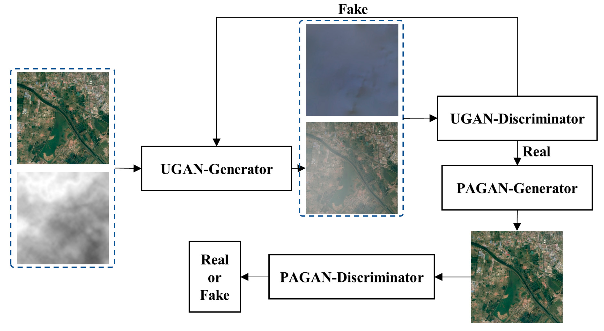
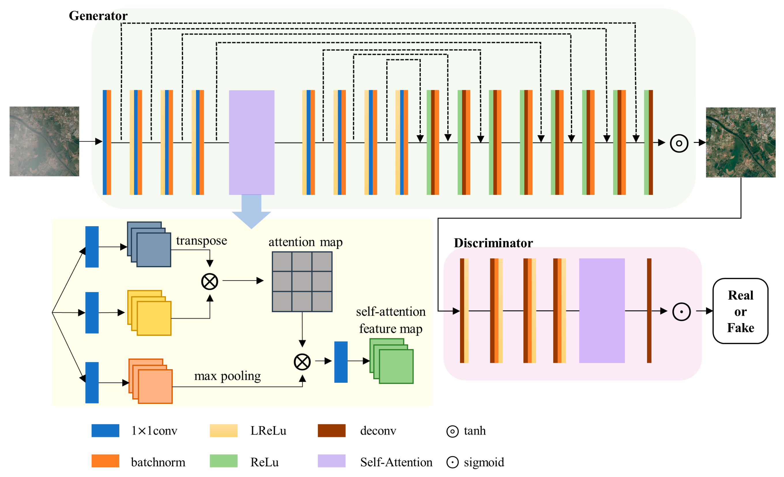
  • A BIS method based on a cascade of GANs including a UGAN and a PAGAN is proposed. The goal of the UGAN is to train a generator that can synthesize new samples following examples of clear images and interference sources. In contrast to the UGAN, the goal of the PAGAN is to train a generator that can separate synthesized images. Moreover, a self-attention module is added to the PAGAN to reduce the difference between the generated image and the ground truth.
  • The organic combination of a synthetic network and a separation network addresses the problem that the training of a deep learning model is difficult due to the lack of paired data.
  • The proposed method is suitable for both natural image separation and remote sensing image separation, and it has an excellent generalization ability.
The rest of the paper is organized as follows. In Section 2, we present the network architectures, including the model structure, loss function, and other details. In Section 3, the evaluation index, datasets, and the experimental results are presented. Finally, Section 4 provides the conclusion and a summary of the results obtained.

2. Materials and Methods

2.1. Overall Architecture
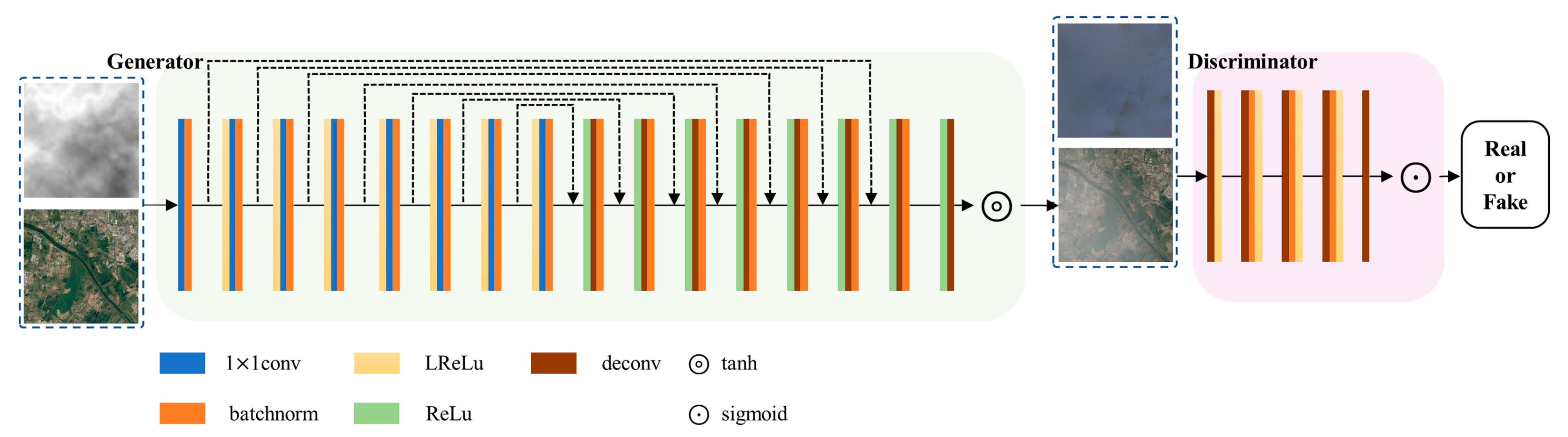
In this section, we describe the architecture of the proposed cascade of GANs and the loss function, and Figure 1 presents the proposed framework and the training process.
As shown in Figure 1, during the training phase, the clear image and interference source are input into the UGAN generator, which generates an image with interference. UGAN’s output image serves as PAGAN’s input, guiding PAGAN to separate the image. The generators in the UGAN and PAGAN modules, respectively generate the corresponding images following distributions that are similar to that of the ground truth so that they are as close to the real image as possible. In the test process, only the PAGAN is required for the BIS task.

2.2. UGAN

The UGAN module simulates the process of disturbing a clear image, and directly generates an image containing the interference source on the clear image. The UGAN comprises a generator and a discriminator, and its structure is shown in Figure 2.
UGAN Generator. The input of the UGAN generator comprises a clear image and an interference source from a common dataset. We use a U-net [19] model as a whole, which includes eight convolution layers and eight deconvolution layers. Each convolution layer has a LReLu layer in front of it and a batchnorm layer behind it except the first one. Similarly, except for the last deconvolution layer, each deconvolution layer has a ReLu layer in front of it and a batchnorm layer behind it. Specifically, to improve the efficiency of the network and better preserve the details of the image, we also concatenate the features at the convolution side to the deconvolution side at each layer. In this way, a mixed image the same size as the input can be generated.
UGAN Discriminator. The purpose of the UGAN discriminator is to ensure that the mixed image generated by the UGAN generator follows the sample distribution of the real mixed image. The main architecture consists of five deconvolution layers. The loss between the ground truth and the generated image is calculated by the loss function. The discriminator determines whether the generated mixed image distribution conforms to the real image distribution, and outputs the possibility that it conforms to the real distribution.

2.3. PAGAN

The goal of PAGAN is to separate the source image from the mixed image more effectively. To achieve this, a self-attention module [20] is added to the network, which improves the convolution efficiency and the ability to capture long-range dependencies. The generator can draw the source from the mixed image, which follows the sample distribution of the real image. The discriminator can discriminate the image drawn by the generator, and in this way, it can ensure that the image drawn by the generator is closest to the real image. The PAGAN structure diagram is shown in Figure 3.
PAGAN Generator. The input of the PAGAN generator is a mixed image. We also use the structure of U-net and skip connection. The self-attention module is added after the fourth convolution module to improve the efficiency of capturing the image dependence by convolution. The self-attention module feeds the self-attention feature map with position feature weights to the next convolution layer, which improves the ability of the convolution layer to capture the remote features. The self-attention module can also implement a global constraint for the image and improve the performance of generation. The output of the PAGAN generator is a clear image the same size as the input image.
PAGAN Discriminator. The discriminator takes the same measures as the generator to capture the detailed remote features of the image, it also incorporates a self-attention module after the fourth deconvolution module. The discriminator determines whether the generated clear image distribution conforms to the real image distribution, and outputs the possibility that it conforms to the real distribution.

2.4. Loss Function

In the training process, we use a generated image and a real image, respectively, to train the GAN generators’ and discriminators’ anti-loss. In addition, in order to improve the performance of the loss function, the L 1 is also used to participate in training [11,21].
Given an observation image X , a random interference vector z and an objective image Y , GAN learns the mapping from X and z to Y , that is, G : { X , z } Y . The process of the UGAN and PAGAN can be expressed as follows:
L GAN ( G , D ) = E X , Y [ log D ( X , Y ) + E X , Y [ log ( 1 D ( X , G ( X , z ) ) ) ] ] ,
where G (the generator) attempts to minimize this objective to generate an image that is more consistent with the true distribution, and D (the discriminator) maximizes the objective to improve its discriminability. The processing of the G and the D with the objective can be expressed as follows:
G * = arg min G max D L GAN ( G , D ) .  
Existing methods prove that it is effective to combine the GAN objective with a traditional loss method, such as L 1 distance [21]. The discriminator only models the high-frequency structures of the image and, on the contrary, the L 1 loss measures the low-frequency structures. The generator is tasked not only with tricking the discriminator but also with generating content near the ground truth output in an L 1 sense, that is:
L 1 ( G ) = E X , Y , z [ Y G ( X , z ) 1 ] .  
The final objective is:
G * = arg min G max G L GAN ( G , D ) + λ L 1 ( G ) ,  
where λ is the weight coefficient of the L 1 loss.

3. Experiments

To test the performance of the method, we selected natural images and remote sensing images as datasets. For the natural image datasets, we compared the results of the proposed method with the results of the classic BIS method, called non-negative matrix factorization (NMF) [5], fast independent component analysis (FastICA) [22], and the state-of-the-art network generation methods, NES and the method of Yang et al. [23]. In the remote sensing image datasets, because of a lack of BIS methods for remote sensing images, we compared the datasets with four dehazing removal methods (the color attenuation prior (CAP) [24], dark channel prior (GDCP) [25], gated context aggregation network (GCANet) [26], and MOF model [15]).

3.1. Evaluation Indices

As evaluation indices, we selected the peak signal-to-noise ratio (PSNR) [27] and structural similarity index (SSIM) [27] for the objective assessment.
PSNR evaluates the pixel difference between the separated image and the real image. The PSNR is defined as follows:
PSNR = 10   ·   log 10 ( M A X I 2 M S E ) = 20   ·   log 10 ( M A X I M S E ) ,  
where M A X I is the maximum value representing the color of the image point; a higher PSNR value indicates a smaller distortion.
From the perspective of image composition, the SSIM regards the structural information as independent of brightness and contrast, which reflects the properties of the object structure in the scene, and the distortion is measured as a combination of three different factors of brightness, contrast and structure. SSIM is defined as follows:
SSIM ( x , y ) = ( 2 μ x μ y + c 1 ) ( 2 σ x y + c 2 ) ( μ x 2 + μ y 2 + c 1 ) ( σ x 2 + σ y 2 + c 2 ) ,  
where μ x is the average of x , μ y   is the average of y , which are estimates of brightness; σ x 2 is the variance of x , σ y 2 is the variance of y , and σ x y is the covariance of x and y , the variance is an estimate of contrast, and covariance is a measure of structural similarity. Moreover, to maintain stability, two constants, c 1 = ( k 1 L ) 2 and c 2 = ( k 2 L ) 2 , are added, L is the dynamic range of pixel values, k 1 = 0.01 , and k 2 = 0.03 The range of the SSIM values is [0, 1].

3.2. Datasets

The natural images are from datasets of shoe and bag images. We selected 1000 images from both the shoe dataset [28] and bag dataset [29] as known samples and performed UGAN processing on the selected images. After processing, 600 images were used as training samples, and 400 images were used as test samples. To test the separation performance of the PAGAN, we also selected 1200 images from both the shoe and bag datasets as known samples and randomly mixed the selected images at a ratio of 7 to 3. In this way, we could test the ability of PAGAN to separate strong sources from synthetic mixed images, and prove the separation performance of the network. Of these images, 1000 were used as training samples and 200 images were used as test samples. For different datasets, we trained models separately for testing.
Because of the potential demonstrated by our method, we further extended our proposed method to the practical application of remote sensing images and conducted experiments on different remote sensing image datasets.
For the remote sensing image datasets, two benchmark datasets from RICE [30] were adopted: RICE-I and RICE-II. RICE-I was collected from Google Earth, and it contained a total of 500 pairs of cloud and corresponding cloudless images with a size of the 512 × 512 pixels [30]. The coverage areas of these images did not overlap each other. The image size in the RICE-II dataset was the same as that in RICE-I, which was 512 × 512 pixels. The RICE-II dataset contained 700 pairs of images without overlapping, and this dataset was part of the Landsat 8 OLI/TIRS dataset [30].

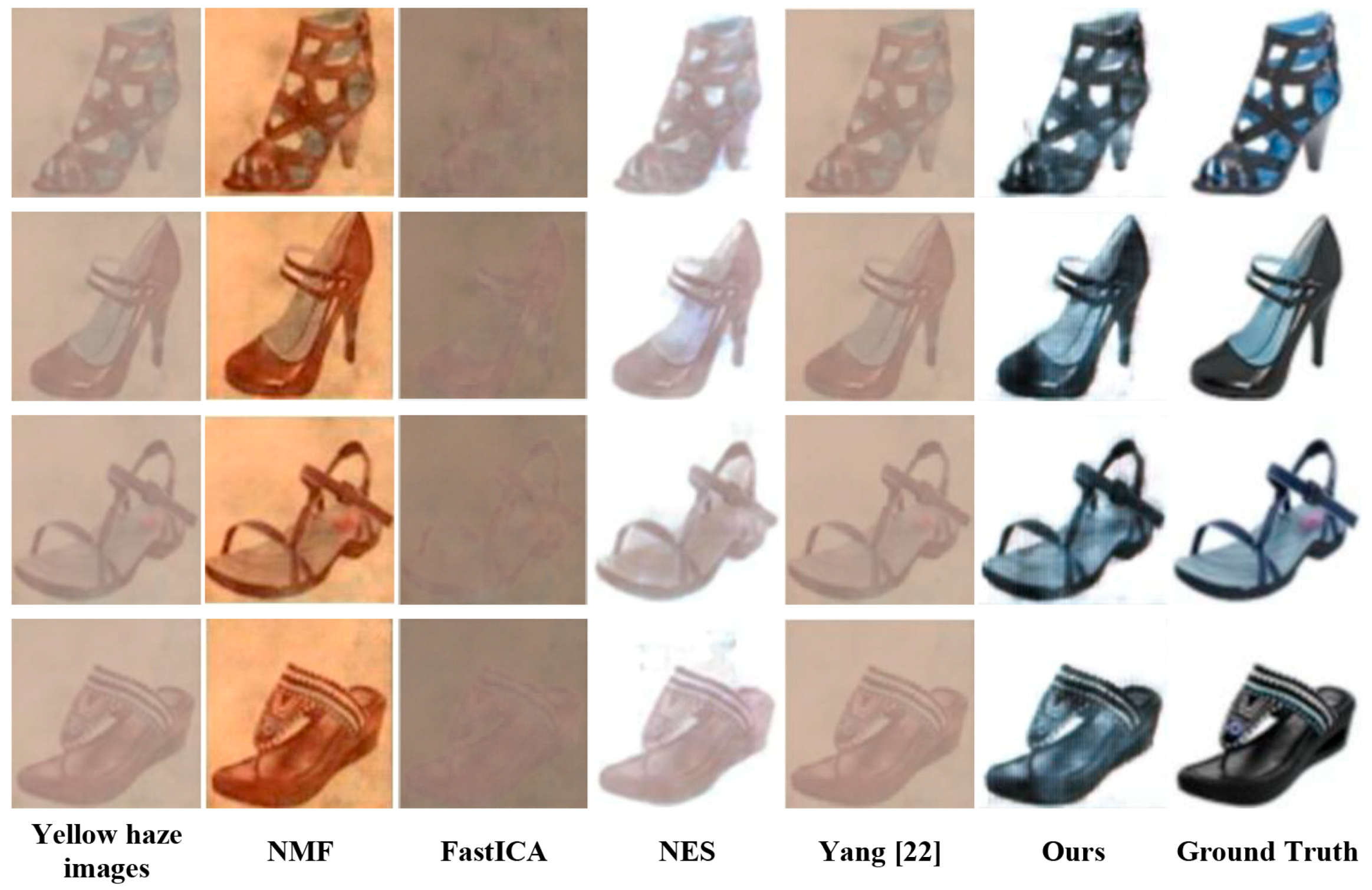
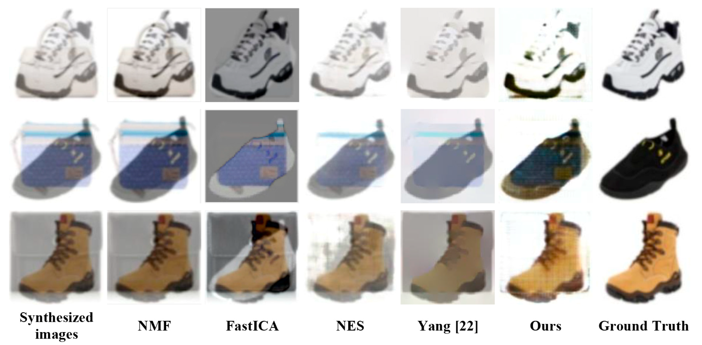
3.3. Experimental Results of the Natural Image Dataset

The UGAN was used to generate the mixed images by adding a yellow haze interference on the clear shoe image source. Next, the generated results were input into the PAGAN to train them to separate the clear shoe image source from the mixed source.
As shown in Figure 4, we see that NMF and FastICA cannot separate the image from the interference source. The single-image reflection removal algorithm proposed by Yang et al. also cannot separate the images. NES can separate the image, but the color is not clear. In contrast, the separation effect of our method is better than those of the other methods.
To further evaluate the separation performance, we carried out experiments on a dataset synthesized from two images. As mentioned before, the purpose of the experiment was to separate the image of the larger weight from the synthetic image. Figure 5 shows three groups of results for the synthetic images. NMF and FastICA were ineffective at separating the two image sources, whereas the NES and single-image reflection removal methods could not clearly separate the image. In contrast, our method achieved better results.
Table 1 lists the objective measurement results for each set of experiments. In Table 1, we can see the PSNR (dB)/SSIM scores of several image separation methods on these two datasets. The separated image is said to be closer to its ground truth if it has a higher PSNR value, while a higher SSIM score means that the result is more similar to its reference image in terms of image brightness, contrast and structure. It can be observed from Table 1 that the proposed method achieves the best performance on two of the datasets, and outperforms NMF, FastICA, NES, and Yang et al.’s method with respect to both PSNR and SSIM. This substantiates the flexibility and generality of our proposed method in diverse mixing types contained in these datasets.

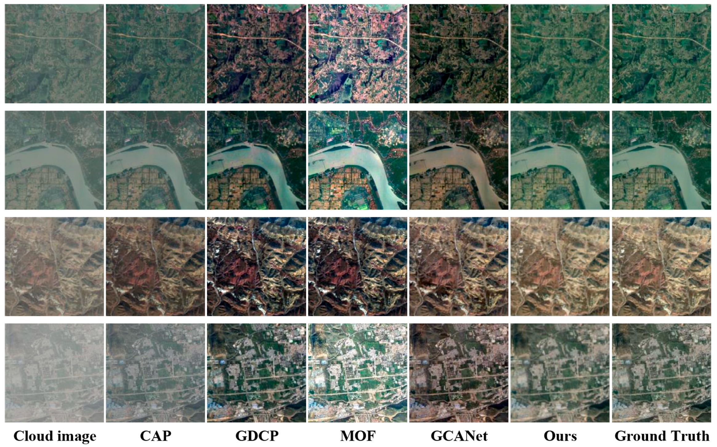
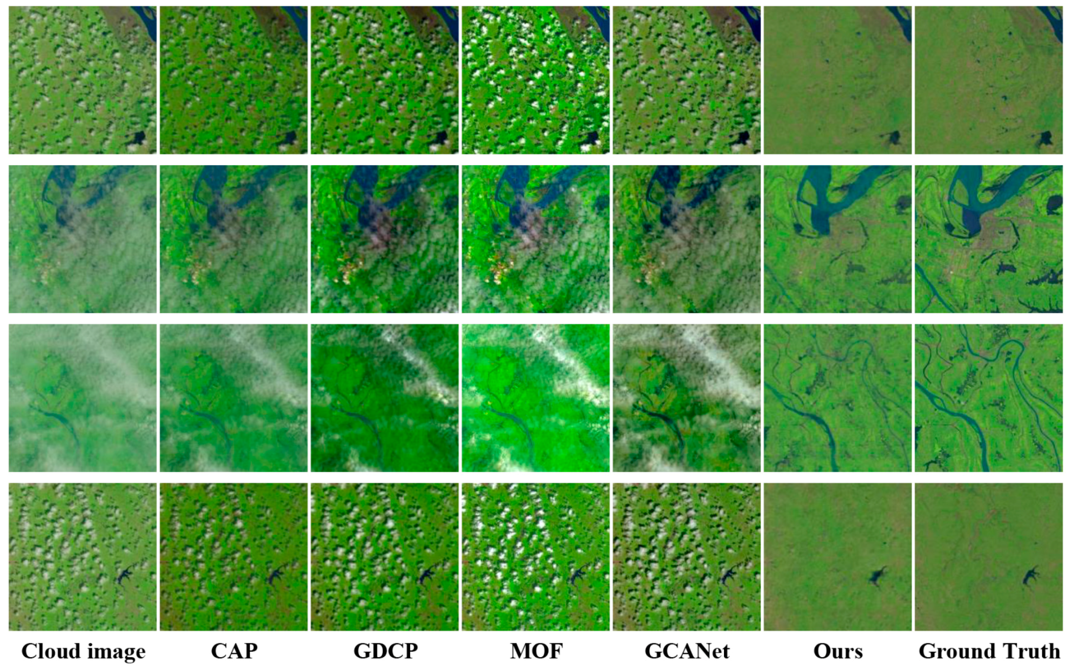
3.4. Experimental Results of the Remote Sensing Image Dataset

Compared with the natural image, the remote sensing image contains more detailed ground information. In the process of acquiring the remote sensing image, due to the atmospheric environment and other reasons, the acquired images are covered by haze and other related shadows; how the images are contaminated is unknown. Therefore, remote sensing image dehaze is an application of BIS.
Qualitative comparisons of the remote sensing image results are shown in Figure 6. The results show that CAP can only reduce part of the haze but cannot remove the haze completely. Especially, the details of the remote sensing image cannot be restored well. The dehazing results of GDCP, MOF and GCANet show that the obtained images have different degrees of spectral distortion, and the original image cannot be accurately restored by the three methods. When compared with other algorithms, the proposed method can better recover the ground truth of the remote sensing image from haze images without spectral distortion.
To further explore the processing of other particles in the atmosphere by the separation method, a comparative removal experiment was performed on the remote sensing image with thin clouds. In contrast to the haze, the clouds had multiple distribution types and different thicknesses. The uncertainty of cloud distribution, thickness, and other information conformed to the characteristics of the blind images [31,32]. Therefore, cloud removal from the remote sensing images was also an image separation problem in the field of BIS. The experimental results are shown in Figure 7. The proposed method effectively reconstructed the information from the clouds and shadows. From the perspective of visual results, it was significantly better than the comparison methods.
A quantitative comparison of the results of dehazing and cloud removal is shown in Table 2. The results show that our method achieves the best values of all comparison methods. Compared to the previous most effective technique, our method achieves a 0.21 improvement in SSIM and 0.18 dB in PSNR in the RICE-II dataset, and achieves a 1.41 dB improvement in PSNR in the RICE-I dataset. This demonstrates that the proposed method better enhances the visibility of the separation scenes under the same mixing components. Therefore, it is suitable for the separation of remote sensing images.

4. Discussion

In this article, we proposed a BIS method based on cascaded GANs that can perform the image separation task without multiple prior constraints. This method uses the UGAN to learn image mixing, which solves the problem of unpaired samples in the training process; the PAGAN is used to learn image separation. The PAGAN module adopts a self-attention mechanism to implement complex geometric constraints on the global image structure more accurately. The proposed method is suitable for different scenes, and extensive experiments demonstrate that it is able to provide competitive and high-quality separation results for both natural images and remote sensing images. In the future, we will continue to explore a unified framework that is more suitable for single-channel BIS and further expand the applicability and portability of this method.

Author Contributions

Formal analysis, F.J., X.S. and Y.M.; methodology, X.S., F.J. and Y.M.; resources, J.X.; data curation, X.S. and F.J.; writing—original draft preparation, F.J. and X.S.; writing—review and editing, J.X. and M.N.; supervision, J.X. and M.N.; funding acquisition, J.X. All authors have read and agreed to the published version of the manuscript.

Funding

This research was funded by the Natural Science Foundation of China, grant number 62072391 and 62066013; the Natural Science Foundation of Shandong, grant number ZR2019MF060; A Project of Shandong Province Higher Educational Science and Technology Key Program, grant number J18KZ016, and the Graduate Science and Technology Innovation Fund Project of Yantai University, grant number YDYB2122.

Institutional Review Board Statement

Not applicable.

Informed Consent Statement

Not applicable.

Data Availability Statement

Conflicts of Interest

The authors declare no conflict of interest.

References

  1. Yang, Z.Z.; Fan, L.; Yang, Y.P.; Yang, Z.; Gui, G. Generalized nuclear norm and Laplacian scale mixture based low-rank and sparse decomposition for video foreground-background separation. Signal Process. 2020, 172, 107527. [Google Scholar] [CrossRef]
  2. Liu, Y.; Lu, F. Separate in latent space: Unsupervised single image layer separation. In AAAI-20 Technical Tracks 7, Proceedings of the AAAI Conference on Artificial Intelligence, New York, NY, USA, 7–12 February 2020. [Google Scholar]
  3. Siadat, M.; Aghazadeh, N.; Akbarifard, F.; Brismar, H.; Öktem, O. Joint image deconvolution and separation using mixed dictionaries. IEEE Trans. Image Process. 2019, 28, 3936–3945. [Google Scholar] [CrossRef] [PubMed]
  4. Hyvärinen, A.; Oja, E. Independent component analysis: Algorithms and applications. Neural Netw. 2000, 13, 411–430. [Google Scholar] [CrossRef] [Green Version]
  5. Cichocki, A.; Mørup, M.; Smaragdis, P.; Wang, W.; Zdunek, R. Advances in nonnegative matrix and tensor factorization. Comput Intel Neurosc. 2008, 2008, 852187. [Google Scholar] [CrossRef] [PubMed]
  6. Pham, D.T.; Garat, P. Blind separation of mixture of independent sources through a quasi-maximum likelihood approach. IEEE Trans. Signal Process. 1997, 45, 1712–1725. [Google Scholar] [CrossRef]
  7. Yu, X.C.; Xu, J.D.; Hu, D.; Xing, H.H. A new blind image source separation algorithm based on feedback sparse component analysis. Signal Process. 2013, 93, 288–296. [Google Scholar]
  8. Xu, J.D.; Yu, X.C.; Hu, D.; Zhang, L.B. A fast mixing matrix estimation method in the wavelet domain. Signal Process. 2014, 95, 58–66. [Google Scholar] [CrossRef]
  9. Goodfellow, I.J.; Pouget-Abadie, J.; Mirza, M.; Xu, B.; Warde, D.; Ozair, S.; Courville, A.; Bengio, Y. Generative adversarial networks. In Proceedings of the 27th International Conference on Neural Information Processing Systems, Montreal, QC, Canada, 8–13 December 2014. [Google Scholar]
  10. Mehdi, M.; Simon, O. Conditional generative adversarial nets. arXiv 2014, arXiv:1411.1784. [Google Scholar]
  11. Isola, P.; Zhu, Y.F.; Zhou, T.H.; Efros, A.A. Image-to-Image translation with conditional adversarial networks. In Proceedings of the IEEE Conference on Computer Vision and Pattern Recognition, Honolulu, HI, USA, 21–26 July 2017. [Google Scholar]
  12. Liu, Y.; Liu, J.; Wang, S. Effective Distributed Learning with Random Features: Improved Bounds and Algorithms. In Proceedings of the 9th International Conference on Learning Representations, Vienna, Austria, 4 May 2021. [Google Scholar]
  13. Li, T.; Lun, D.P.K. Single-image reflection removal via a two-stage background recovery process. IEEE Signal Process. Lett. 2019, 26, 1237–1241. [Google Scholar] [CrossRef]
  14. Halperin, T.; Ephrat, A.; Hoshen, Y. Neural separation of observed and unobserved distributions. In Proceedings of the Machine Learning Research, Proceedings of the 36th International Conference on Machine Learning, Long Beach, CA, USA, 9–15 June 2019. [Google Scholar]
  15. Zhao, D.; Xu, L.; Yan, Y.; Chen, J.; Duan, L.Y. Multi-scale optimal fusion model for single image dehazing. Signal Process. Image Commun. 2019, 74, 253–265. [Google Scholar] [CrossRef]
  16. Sun, X.; Xu, J.D.; Ma, Y.L.; Zhao, T.; Ou, S.; Peng, L. Blind image separation based on attentional generative adversarial network. J. Ambient Intell. Hum. Comput. 2020, 3, 1–8. [Google Scholar] [CrossRef]
  17. Cai, B.; Xu, X.; Jia, K.; Qing, C.; Tao, D. Dehazenet: An end-to-end system for single image haze removal. IEEE Trans. Image Process. 2016, 25, 5187–5198. [Google Scholar] [CrossRef] [PubMed] [Green Version]
  18. Shen, H.; Li, X.; Cheng, Q.; Zeng, C.; Yang, G.; Li, H.; Zhang, L. Missing information reconstruction of remote sensing data: A technical review. IEEE Geosci. Remote Sens. Mag. 2015, 3, 61–85. [Google Scholar] [CrossRef]
  19. Wu, C.; Zou, Y.; Zhi, Y. U-GAN: Generative Adversarial Networks with U-Net for Retinal Vessel Segmentation. In Proceedings of the 2019 14th International Conference on Computer Science Education, Toronto, ON, Canada, 19–21 August 2019. [Google Scholar]
  20. Zhang, H.; Goodfellow, I.J.; Metaxas, D.; Odena, A. Self-Attention generative adversarial networks. In Proceedings of the Machine Learning Research, Proceedings of the 36th International Conference on Machine Learning, Long Beach, CA, USA, 9–15 June 2019. [Google Scholar]
  21. Zhao, H.; Gallo, O.; Frosio, L.; Kautz, J. Loss functions for image restoration with neural networks. IEEE Trans. Comput. Imaging 2017, 3, 47–57. [Google Scholar] [CrossRef]
  22. Hesse, C.W.; James, C.J. The fastica algorithm with spatial constraints. IEEE Signal Process. Lett. 2005, 12, 792–795. [Google Scholar] [CrossRef]
  23. Yang, Y.; Ma, W.; Zheng, Y.; Cai, J.F.; Xu, W. Fast single image reflection suppression via convex optimization. In Proceedings of the IEEE Conference on Computer Vision and Pattern Recognition, Long Beach, CA, USA, 15–20 June 2019. [Google Scholar]
  24. Zhu, Q.; Mai, J.; Shao, L. A fast single image haze removal algorithm using color attenuation prior. IEEE Trans. Image Process. 2015, 24, 3522–3533. [Google Scholar] [PubMed] [Green Version]
  25. He, K.; Sun, J.; Tang, X. Single image haze removal using dark channel prior. IEEE Trans. Pattern Anal. Mach. Intel. 2011, 33, 2341–2353. [Google Scholar]
  26. Chen, D.; He, M.; Fan, Q.; Liao, J.; Zhang, L.; Hou, D.; Yuan, L.; Hua, G. Gated context aggregation network for image dehazing and deraining. In Proceedings of the 2019 IEEE Winter Conference on Applications of Computer Vision, Waikoloa, HI, USA, 7–11 January 2019. [Google Scholar]
  27. Horé, A.; Ziou, D. Image quality metrics: PSNR vs. SSIM. In Proceedings of the 2010 20th International Conference on Pattern Recognition, Istanbul, Turkey, 23–26 August 2010. [Google Scholar]
  28. Zhu, J.Y.; Krähenbühl, P.; Shechtman, E.; Efros, A.A. Generative Visual Manipulation on the Natural Image Manifold. In Proceedings of the Computer Vision-ECCV 2016, European Conference on Computer Vision, Amsterdam, The Netherlands, 11–14 October 2016. [Google Scholar]
  29. Yu, A.; Grauman, K. Fine-grained visual comparisons with local learning. In Proceedings of the IEEE Conference on Computer Vision and Pattern Recognition, Columbus, OH, USA, 23–28 June 2014. [Google Scholar]
  30. Lin, D.; Xu, G.; Wang, X.; Wang, Y.; Sun, X.; Fu, K. A remote sensing image dataset for cloud removal. arXiv 2019, arXiv:1901.00600. [Google Scholar]
  31. Zhang, Y.; Guindon, B.; Cihlar, J. An image transform to characterize and compensate for spatial variations in thin cloud contamination of Landsat images. Remote Sens. Environ. 2002, 82, 173–187. [Google Scholar] [CrossRef]
  32. Shan, S.; Wang, Y. An algorithm to remove thin clouds but to preserve ground features in visible bands. In Proceedings of the IGARSS 2020-2020 IEEE International Geoscience and Remote Sensing Symposium, Waikoloa, HI, USA, 26 September–2 October 2020. [Google Scholar]
Figure 1. Proposed framework and training process.
Applsci 11 09416 g001
Figure 2. UGAN structure.
Applsci 11 09416 g002
Figure 3. PAGAN structure.
Applsci 11 09416 g003
Figure 4. Results of image separation for the yellow haze images.
Applsci 11 09416 g004
Figure 5. Result of image separation for synthesized images.
Applsci 11 09416 g005
Figure 6. Results of the RICE-I dataset for image dehazing.
Applsci 11 09416 g006
Figure 7. Results of the RICE-II dataset for cloud removal.
Applsci 11 09416 g007
Table 1. Shoe and bag image results (PSNR, SSIM).
PSNR (dB)/SSIMNMFFastICANESYang [22]Ours
Yellow haze images15.02/0.4212.67/0.1519.75/0.6315.70/0.4525.92/0.89
Synthesized images23.79/0.7014.70/0.5520.56/0.7821.37/0.7123.84/0.88
Table 2. Remote sensing image results (PSNR, SSIM).
PSNR (dB)/SSIMCAPGDCPMOFGCANetOurs
RICE-I24.51/0.8220.35/0.8316.64/0.7319.93/0.8025.92/0.85
RICE-II20.97/0.6117.18/0.5418.04/0.4819.16/0.5621.15/0.82
Publisher’s Note: MDPI stays neutral with regard to jurisdictional claims in published maps and institutional affiliations.

