Data-Driven Convolutional Model for Digital Color Image Demosaicing

Abstract

Modern digital cameras use specific arrangement of Color Filter Array to sample light wavelength corresponding to visible colors. The most common Color Filter Array is the Bayer filter that samples only one color per pixel. To recover the full resolution image, an interpolation algorithm can be used. This process is called demosaicing and it is one of the first processing stages of a digital imaging pipeline. We introduce a novel data-driven model for demosaicing that takes into account the different requirements for reconstruction of the image Luma and Chrominance channels. The final model is a parallel composition of two reconstruction networks with individual architecture and trained with distinct loss functions. In order to solve the overfitting problem, we prepared a dataset that contains groups of patches that share common chromatic and spectral characteristics. We reported the reconstruction error on noise-free images and measured the effect of random noise and quantization noise in the demosaicing reconstruction. To test our model performance, we implemented the network on NVIDIA Jetson Nano, obtaining an end-to-end running time of less than one second for a full frame 12 MPixel image.

1. Introduction

Modern digital cameras capture images using a single Charge-Coupled Device (CCD) or Complementary Metal–Oxide–Semiconductor (CMOS) array of photosensors arranged in a rectangular matrix. Between the light source and the photosensor, a color film or dye filters the light in some limited frequency bandwidth. The overall effect is that each sensor is able to register the intensity of the light for a single primary color (Red, Green, or Blue). The specific arrangement of such color filters is called a Color Filter Array (CFA). By far the most common CFA arrangement in commercial cameras is the Bayer filter array [1]. A Bayer filter array is a repetitive matrix of 2 × 2 tiles that spans the entire sensor surface. In a Bayer filter, each sensor corresponds to an image pixel; this implies that, since each sensor captures the light intensity for a single color channel, at each pixel location in the output image only a single intensity value is available per channel. Typically green pixels are sampled more often then red and blue pixels, although the ordering of the 2 × 2 arrangement of pixels may change between sensor manufactures (Figure 1). Green pixels are sampled more often then red and blue pixels because the human eye is more sensitive to variations in intensity in the middle of the visible light spectrum that roughly correspond to green wavelengths. For this reason, the green channel is generally used to approximate the perceived image brightness (Luma Channel), whereas the red and blue channels are used to reconstruct the original input image color (Chrominance Channel). Other filter arrangements are possible and some have been proposed specifically to improve on the shortcomings of Bayer filters, however these arrangements are often more difficult to manufacture and are far less common in commercial cameras [2,3,4,5].

The main consequence of using a Bayer filter to produce a three-channel color image is that each color channel is effectively downsampled and interpolation is required to recover the original image. When applied to Bayer filters, this interpolation is called “Demosaicing” as it reconstruct the three color channels from the raw input image acquired using the Bayer filter array mosaic of 2 × 2 tiles. Demosaicing algorithms estimate the missing red, green, and blue pixels based on the available input raw image data in order to produce an output image that is visually similar to the original full-resolution color image. Since only partial information is available, it is in general not possible to recover the exact image without introducing some errors. Some assumptions can made to constraint the problem and allow an algorithm to find a unique solution; however, when such assumptions are not valid, artifacts in the output image appear. Two main classes of such artifacts frequently addressed in the literature are the “zipper effect” and “false colors”. The zipper effect appears as abrupt or unnatural changes of intensities over neighboring pixels. That is, the contribution of each color plane to the reconstruction of one pixel differs from that of its immediate neighboring pixel, consequently imposing an artificial repetitive pattern to the output. False colors are spurious colors in the output image that were not present in the original image. Clearly, such visual artifacts decrease the quality of the output image and should be avoided or at least reduced (examples of zipper effect and false colors artifacts are shown in Figure 2).

Noise in the raw input image also poses serious challenges as it propagates in the demosaicing algorithms producing visual artifacts in the output image. For this reason, recent research works have included raw input image denoising as a pre-processing step in their algorithms, improving the final output image quality [7]. Image Demosaicing is still an active research field, as the underlying interpolation problem is far from being solved. New algorithms that use technology and models that were not available in early research works have been published recently, confirming the interest in developing resource-efficient techniques to improve the quality of reconstruction.

The main objective of this paper is to present a novel processing model to perform combined raw image denoising and demosaicing. Given the vast amount of literature, we selected a subset of assumptions that have proved to enhance the output image quality and embedded in our model. We also assume a certain degree of model variability by letting some model parameters to be learned offline from a dataset of natural image patches. We then compress our model to improve its portability to resource-constraint embedded devices and provide a case study implementation of the model for NVIDIA Jetson Nano.

The rest of the paper is organized as follows. In Section 2 we summarize some of the algorithms that have proven to be effective in reconstructing the original input image or that have significant computational advantages. A more detailed description is given for those algorithms we selected to be included in our model. In Section 3 we give a detailed description of our model and justify some of its underlying assumptions. In Section 4 we compare our solution to other algorithms presented in the literature on a number of challenging datasets. The effect of model compression is evaluated and a proper trade-off between image quality and computational cost is selected. Running time metrics are reported for the Jetson Nano implementation of the algorithm. Final conclusions are drawn in Section 5.

2. Previous Works

First attempts at solving the demosaicing problem assume channel independence, meaning that each color channel is processed independently. The Nearest-Neighbor algorithm “recovers” the missing data by simply copying the value of the pixel at the closest location. Although computationally efficient, the Nearest-Neighbor algorithm leverages too simplistic assumptions that are generally not met in natural images, thus producing visible artifacts in the output reconstruction. To compensate the limitations of the Nearest Neighbor interpolation, Bilinear interpolation was proposed in the early 1980s. In the Bilinear interpolation algorithm, missing values are recovered by linear interpolation of the available channels in both vertical and horizontal directions. Such linear interpolation can be effectively implemented on Digital Signal Processors (DSPs), as it is realized by convolving the input image with appropriate kernels [8]. The Bilinear interpolation algorithm is effective in areas with homogeneous colors, but it fails in areas containing high frequency components (textures and edges), producing false colors and zippering effect along the boundaries between regions of different colors. Higher order interpolations are possible (i.e., Bicubic interpolation), but they require more computational power and may still produce visible artifacts. Higher quality results can be achieved if inter-channel correlation is taken into account. Specifically, natural images exhibit high level of Spectral correlation and Spatial correlation. In [9], authors show high correlation among the three color components in natural images, especially in high frequency areas. Similarly, natural images are highly spatially correlated: pixels that are spatially close together also have similar color values. Clearly, this assumption fails at the boundary between two different objects, and consequentially algorithms that assume spatial correlation require additional information about the edges in the image in order to suppress the interpolation in the proximity of the boundary between two different homogeneous regions. Two main assumptions are frequently adopted in the literature regarding spectral correlation [10]: the first assumption assumes a constant color difference, and the second assumes constant color ratio. Formally, given that R, G, and B, respectively, are the red, green, and blue channel in the input image, the constant color difference states that: $I_i-I_j=constanti,j\in {\{R,G,B\}}^2$, whereas the constant color ratio assumes $I_i/I_j=constanti,j\in {\{R,G,B\}}^2$. Since the difference between color components is numerically more stable than their ratio and it produces similar results, we will use the constant color difference assumption for the rest of this paper. Both assumptions becomes invalid at the boundaries between regions, that is, the reconstruction fails if two pixels belonging to different objects are mixed in the interpolation. This scenario can be avoided if missing components are estimated along the edges between two homogeneous regions rather than across it. Based on this result, gradient-based methods have been used to guide the interpolation direction according to the edge orientation. The Hibbard method [11] selects the interpolation direction based on the relative strength of the horizontal and vertical gradient on the green channel. If horizontal edges are in magnitude stronger then vertical edges, the reconstruction is the mean of the vertical pixels, whereas if the vertical edges are in magnitude stronger than horizontal edges, the estimated value is the mean of the horizontal pixels. The mean of the four adjacent pixels is used in estimating the pixel, if the vertical and horizontal edges have the same magnitude. Although the original implementation is based on a 3 × 3 neighborhood, larger neighborhoods have been proposed, as well as higher order derivatives [12]. Green color reconstruction based on filter banks and optimal filter design have been proposed in [13,14]. Approximate horizontal and vertical gradients have poor results in regions with high frequency components. Based on the assumption that direction is always detected correctly, when this is not the case, visible artifacts appear.

An alternative solution is to identify template-based feature in order to direct the interpolation according to the locally encountered feature. This class of algorithms is called template-matching based methods [10,15]. In [10], authors classify three classes of features: edges, stripes, and corners, and select a different interpolation strategies according to the locally detected feature. This approach has, however, some serious limitations: it is in general difficult to explicitly define the characteristics of a template, and it may be sensitive to noise, geometrical distortions, and changes in the illumination. In [15], authors implement a template-based demosaicing scheme by applying template matching on the color difference planes $R-G$ and $B-G$, thus effectively combining spatial and spectral correlations. Although color difference planes have less high-frequency information than single component planes, they can still provide the relevant edge information required for correct demosaicing.

Adaptive methods solve the demosaicing problem by locally weighting the available color information by a normalized factor as a function of the directional gradient [16]. Various weighting strategies are possible and explored in [14,17]. Although this class of methods may provide qualitative interesting results, they require more computational overhead as the weights are constantly updated when processing the image.

Frequency domain methods are based on the observation that the mosaic image produced by the Color Filter Array is a sampling process, thus it can be studied in the context of Digital Signal Processing. Images are processed by a filter bank that decomposes the input image in low frequency components and high frequency components. A signal reconstruction process is then applied to each one of the extracted frequency components [18,19].

Modern solutions to the demosaicing problem are data-driven approaches based on variations of classical Convolution Neural Network architectures. In [20], authors study the effectiveness in applying Convolutional Neural Networks (CNN) to solve reconstruct images. However, in [7], authors jointly solve the demosaicing as well as image denoising by training a Deep Neural Network model. Deep Residual Neural Networks for image reconstruction have been studied in [21], reporting high quality results. The main issue with data-driven models is the possibly large number of parameters required to achieve low reconstruction error. Although a larger number of parameters allow the model to correctly reconstruct the original image, it also increases its computational cost and memory requirements.

The rich literature on demosaicing comprises a multitude of insights, methods, and assumptions. In this work, we designed our algorithm by combining some of these assumptions and observations with a data-driven approach. We specifically included in our design the Constant Color Difference [8] and the local edge information [16]. Nevertheless, we recognize the possibility that these assumptions may be violated for some specific regions of the image, and therefore let the model adjust its internal parameters by training offline on different datasets. We also used a custom loss function to reduce the visibility of reconstruction artifacts.

3. Methods

The emerging general agreement from previous works on demosaicing is that any effective demosaicing algorithm should take advantage of both spatial correlation between color pixel of the same channel (intraplane correlation) and spectral correlations among channels (interplane correlation) [14,22]. Local features are also very important for the reconstruction process [10,17], as they are used by the algorithm to identify the main gradient direction in a local patch and drive the interpolation direction along its orthogonal direction to better preserve local edge structures. When applied to the whole image, the overall effect is a sharper image with less blurring.

Additionally, some assumptions about the data can be included in the model as possible data distribution priors [8]. However, these assumptions about the data distribution are in general not sufficient to reconstruct images without introducing visible artifacts when the underlying modeling assumptions are not met. Data-driven approaches can be used to overcome such limitations as the model parameters can be adapted to the data using a learning process (offline learning). There still exists the important underlying assumption that a fixed model structure is selected a priori and only the model parameters are allowed to change during training. This is in general not a limitation given that the model is complex enough to capture the relation between input and outputs. It is however, by definition, the “best” model (selected from the class of possible models with the given fixed structure) for the data present in the training dataset. If the “real” input data are different from the training data, the model may not be able to generalize, and it can produce very poor results. This is the effect of model overfitting on the training data and it can be mitigated with a variety of different strategies.

The Demosaicing interpolation process is defined as the generation of an estimate image from the input Bayer image, such that the estimate image is visually as close as possible to the original RGB image. Formally:

$$\underset{\mathit{\theta }}{min}∥demosaicing(\mathit{\theta },I_{Bayer})-I_{rgb}∥$$

(1)

where $I_{Bayer}$ is the input image with the Bayer Color Filter Array, $I_{rgb}$ is the original RGB image and $\mathit{\theta }$ is the set of parameters required by the demosaicing algorithm, and the $∥·∥$ is a generic distance function.

The main issue in the previous problem formulation is the difficult selection of the distance function that describes the visual similarity between the two images. Different distance functions have been explored in the literature (e.g., Mean Squared Error, Mean Absolute Error, Structural Similarity Index) but no general consensus has been achieved, since image visual similarity is often a subjective evaluation. Nevertheless, a collection of input/output patches can be used to learn a local mapping function from a Bayer patch to a RGB patch. The learned function can be then applied to the whole image. However, learning a function from a set of input/output examples can lead to model overfitting that poses serious issues in the demosaicing reconstruction process. For the original Kodak dataset, the overfitting problem is significant as some images may contain a large number of visually similar patches (most of them have low frequency green and brown components). To overcome this problem, we defined a data selection strategy to extract patches with different chromatic and spectral characteristics from a set of input images.

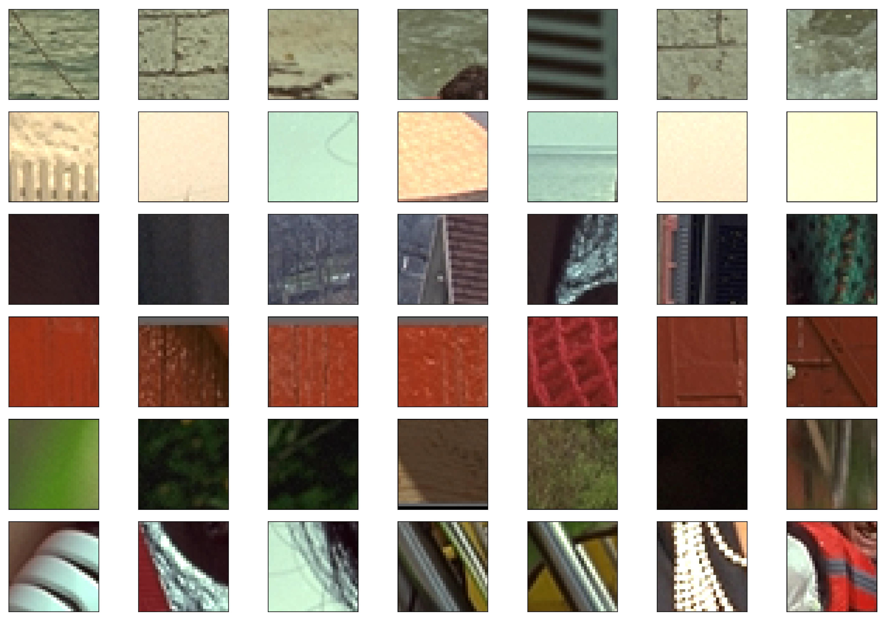
3.1. Dataset Creation

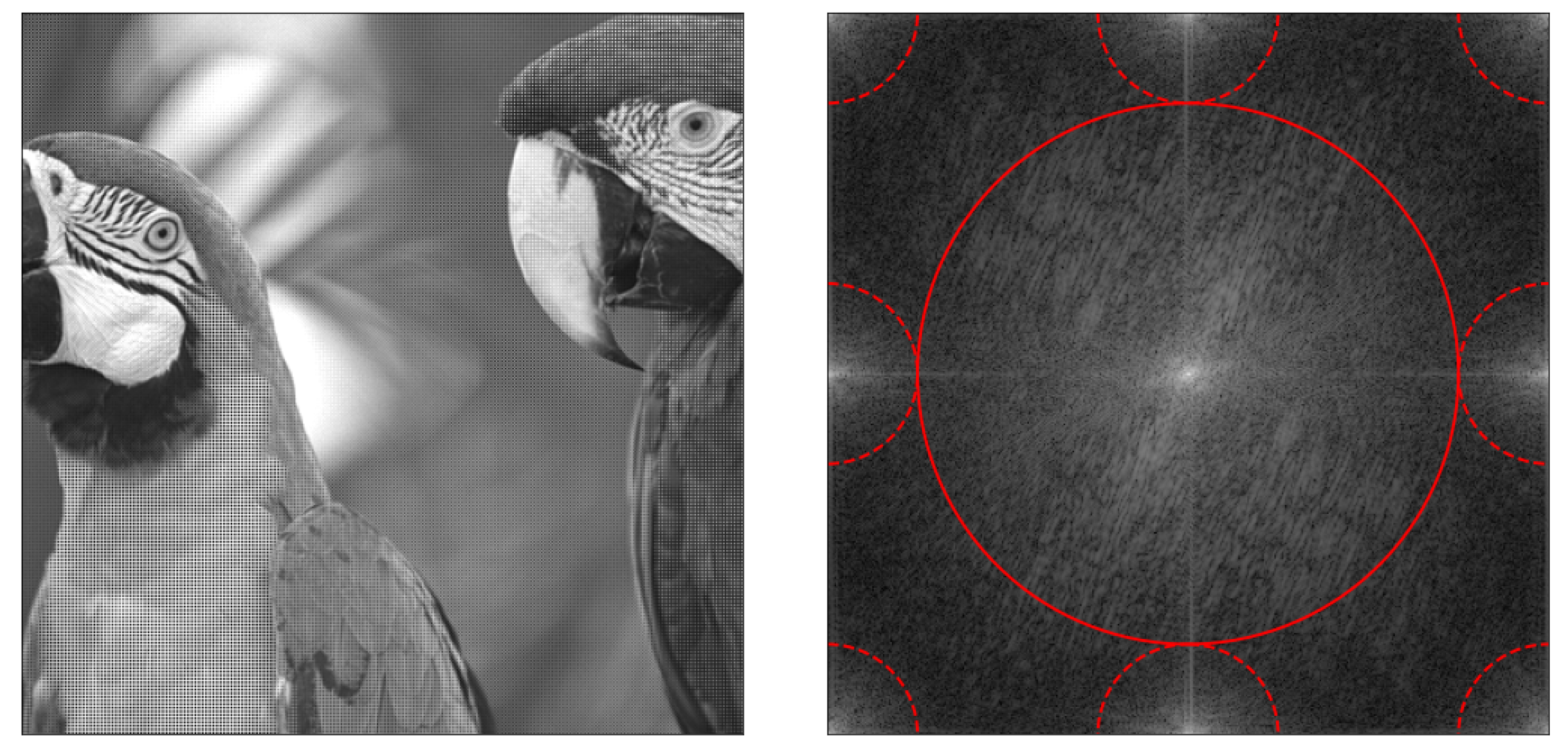
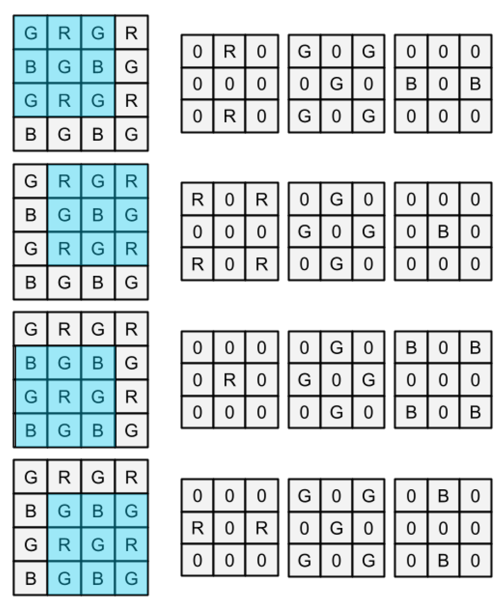
As discussed previously, any demosaicing algorithm can be interpreted as an interpolation problem that estimates a three-channel RGB image from a Bayer image (the image produced by the camera sensor through the Bayer Color Filter Array). In the entire acquisition process, three images can be identified: the real image (the collection of light wavelengths that pass through the camera lenses), the Bayer image (the image as registered by the camera sensor), and the reconstructed image (the RGB image reconstructed by the demosaicing algorithm). It is evident that exact reconstruction of the real image is not possible, as multiple processing steps drop a significant amount of the original information contained in the input signal. In particular, light wavelengths are quantized by the digital camera sensor and various sources of electrical noise can corrupt the registered signal that passes through the Bayer filter. Moreover, the Bayer filter itself is a sampling process that is unable to register spatial color variations that occur at distances smaller then the pixel unit. It is therefore acceptable to obtain a reconstructed image that is an estimate of the real image within a given level of tolerance. Generally, demosaicing algorithms are tuned to produce reconstructed images that are “visually pleasing”, meaning that they tend to have a low number of visible artifacts and do not appear blurred.

In principle, demosaicing interpolation estimates the full-resolution three-channel input image from the single channel Bayer image, however it is usually very difficult to obtain the original input image, as specialized sensors are required to register each color channel as a full-resolution image. It is instead much more common in the literature to simulate the effect of the Bayer filter by sampling a RGB image. The input RGB image is effectively an image that has been already reconstructed by the demosaicing algorithm executed by the camera firmware, thus it is not exactly the same reconstruction process; it is, however, considered a valid approximation of the real process (to overcome this limitation, in [23] authors propose a datasets containing real-color images acquired with specialized hardware). Similarly to other works in the literature, we simulated the Bayer images by sampling RGB images with a specific Bayer Color Filter Array configuration. Other Bayer configurations produce different datasets.

A Bayer image can be obtained by an input RGB image by applying spatial sampling functions for the specific Bayer Configuration (see Figure 3). For other Bayer filter configurations, similar functions can be defined.

All this considered, we used the following procedure to create the patch dataset used to train our demosaicing model. First, we randomly selected 10 full-resolution images from the Kodak dataset [6], leaving the other 10 images as validation data. For each image in the selected collection, we generated a large array of random positions that we iterate to extract the corresponding patches from the RGB image. The generated random positions are all aligned such that we extract patches in the Bayer image with the same Bayer configuration. Therefore, for each RGB image we collect a large number of patches extracted from different locations in the image. On this intermediate collection, we applied a clustering algorithm to group similar patches (in our work we used k-means, but other clustering strategies are possible). We defined a set of features to be used by the clustering algorithm to group similar patches in the same cluster. We represented each patch as a vector of its main chromatic and spectral features: mean saturation value, mean hue, mean luminosity, mean edge magnitude, weighted edge direction. It is relevant to highlight that this feature extraction process has been used only to group similar patches for the purpose of dataset creation, and it is not required for the actual reconstruction algorithm. After clustering, each patch is assigned to a group of patches with similar characteristics.

We compared DBSCAN, Spectral Clustering, and K-means as possible candidates for the patch grouping algorithm, but obtained similar grouping with no apparent differences. Thus, given the low data dimensionality of the patch descriptors, we selected the k-means clustering for patch grouping as it is based on assumptions compatible with the statistics of the input data and it is known to scale well for large numbers of samples. An arbitrary value of K between 10–20 can be selected in order to obtain clusters with visually coherent patches (reported results are relative for K = 15). In k-means clustering, the number of clusters has to be defined beforehand. However, some images may not exhibit large patch diversity, therefore different clusters can contain patches that are in practice very similar. We solved this issue by imposing the additional condition that multiple clusters can be merged if the distance between their centroids is less than a given threshold. The final training dataset is obtained by sampling a given number of random patches from each group of patches (we used the number of elements in the smallest cluster as the number of random samples). This strategy allowed us to create a rich dataset of patches with different chromatic and spectral characteristics that are common in natural images. A similar approach can be used for synthetic images as well.

The complete dataset creation process is depicted in Figure 4.

From the Kodak dataset [6], we extracted a dataset consisting of 56,000 patches. We provide some representative samples for different groups of patches in Figure 5. From the reported samples, the diversity among the classes of patches can be appreciated.

3.2. Image Model

As in [19], we define a color image I as a mapping function from discrete coordinate $(x,y)$ to a three-dimensional RGB color vector.

$$I(x,y)=\{C_r(x,y),C_g(x,y),C_b(x,y)\}$$

(2)

We can also define a suitable projection in the RGB space as a positive combination of color components. This projection allows us to express the original input three-dimensional image as the sum of a scalar channel and a vector of residuals. Formally,

$$I(x,y)=\{C_r(x,y),C_g(x,y),C_b(x,y)\}=\Phi (x,y)+\left\{{\Psi }_i(x,y)\right\},i\in \{R,G,B\}$$

(3)

where $\Phi (x,y)$ is a scalar (one-dimensional) image and $\left\{{\Psi }_i(x,y)\right\}=\{C_i(x,y)-\Phi (x,y)\}$ is a three-dimensional vector of residuals. If we project the image on to the vector $[1/3,1/3,1/3]$, the scalar image is effectively the Luminance channel (i.e., the pixel-wise mean among the color channels) and the residual vector is the Chrominance channel.

Similarly, we can define the Bayer image as the input image spatially subsampled by specific masking function for each color channel. Formally,

$$I_{Bayer}(x,y)=\{C_r(x,y)m_R(x,y),C_g(x,y)m_G(x,y),C_b(x,y)m_B(x,y)\}$$

(4)

where $m_R$, $m_G$, and $m_B$ are three masking cosine functions defined for each possible Bayer configuration. For the Bayer RGGB configuration, $m_R$, $m_G$, and $m_B$ are defined as follows:

$$\begin{array}{cc}\hfill m_R(x,y)& =\frac{1}{4}(1+cos(\pi x))(1+cos(\pi y))\hfill \\ \hfill m_G(x,y)& =\frac{1}{2}(1-cos(\pi x)cos(\pi y))\hfill \\ \hfill m_B(x,y)& =\frac{1}{4}(1+cos(\pi x+\pi ))(1+cos(\pi y+\pi ))\hfill \end{array}$$

(5)

For Bayer images, it is relevant to analyze their Fourier Transform as it provides useful information that can drive the reconstruction process. Given the Bayer image representation in (4), its Fourier transform can be defined as the convolution in the frequency domain of the Fourier transform for each color channel ${\widehat{C}}_i(u,v)$ and the Fourier transform of the sampling functions ${\hat{m}}_i(u,v)$ (6). The Fourier transform of the Bayer image can thus be expressed as:

$${\widehat{I}}_{Bayer}(u,v)=\sum _i{\widehat{C}}_i(u,v)\ast {\hat{m}}_i(u,v)$$

(6)

Since the sampling functions are based on cosine functions, their Fourier transform are Dirac delta functions localized at different positions in the frequency spectrum. Thus, as the convolution with a Dirac delta functions is a translation of the original signal in the frequency spectrum ${\widehat{C}}_i(u,v)\ast \delta (u_0,v_0)={\widehat{C}}_i(u-u_0,v-v_0)$, the sampling functions localize the Chrominance and Luminance of the input image in the frequency spectrum. By expansion of Equation (6), the Fourier transform of the spatially subsampled input image can be expressed as:

$$\begin{array}{cc}\hfill {\widehat{I}}_{Bayer}(u,v)& =\sum _{i\in \{R,G,B\}}{p}_i{\widehat{C}}_i(u,v)\hfill \\ \hfill & +\sum _{(u,v)\in \{(-1,-1),(1,-1),(1,1),(-1,1)\}}\frac{1}{8}({\widehat{C}}_R(u,v)-{\widehat{C}}_B(u,v))\hfill \\ \hfill & +\sum _{(u,v)\in \{(0,-1),(1,0),(0,1),(-1,0)\}}\frac{1}{16}({\widehat{C}}_R(u,v)-2{\widehat{C}}_G(u,v)+{\widehat{C}}_B(u,v))\hfill \end{array}$$

(7)

As observed in [19], the Bayer sampling applied to the input image creates aliasing in nine distinct regions of the spectrum (see Figure 6). Most of the Luminance energy is concentrated in the central region, whereas the Chrominance energy is located at the borders. In Figure 6, the Fourier transform of the Bayer image is presented. From the image, nine regions can be identified where most of the energy is concentrated, these correspond to each of the members in (7).

From the Fourier representation of the Bayer image, four categories of visual artifacts generated in the reconstruction process can be explained (i.e., blurring, grid effect, false color, and watercolor). Blurring can be generated if the estimation of the Luminance spectrum is too narrow, hence all the high frequency components of the input signal are suppressed. The grid effect artifact is due to selection of a wider band that might include Chrominance components in the Luminance signal. Similarly, if the bandwidth of the filter allows the Luminance component to spill in the Chrominance signal, the false color artifact is visible. Finally, if the Chrominance filter bandwidth is too narrow, low frequency components in the Chrominance channel causes the color of the objects to spread beyond their edges thus producing a visible watercolor effect. Classical demosaicing algorithms tend to underestimate Luminance and overestimate Chrominance, therefore blurring and false color artifacts are particularly evident.

Optimal selection of the bandwidth for the chrominance and Luminance filters is, in general, not possible as it depends on the original input signal. In this work we propose a data-driven solution to this problem, by learning the filter coefficients that minimize a cost function on the training dataset of patches. With this approach, we let the network act as a non-linear filter with learnable coefficients that can automatically select the “best” separation between regions in the frequency spectrum.

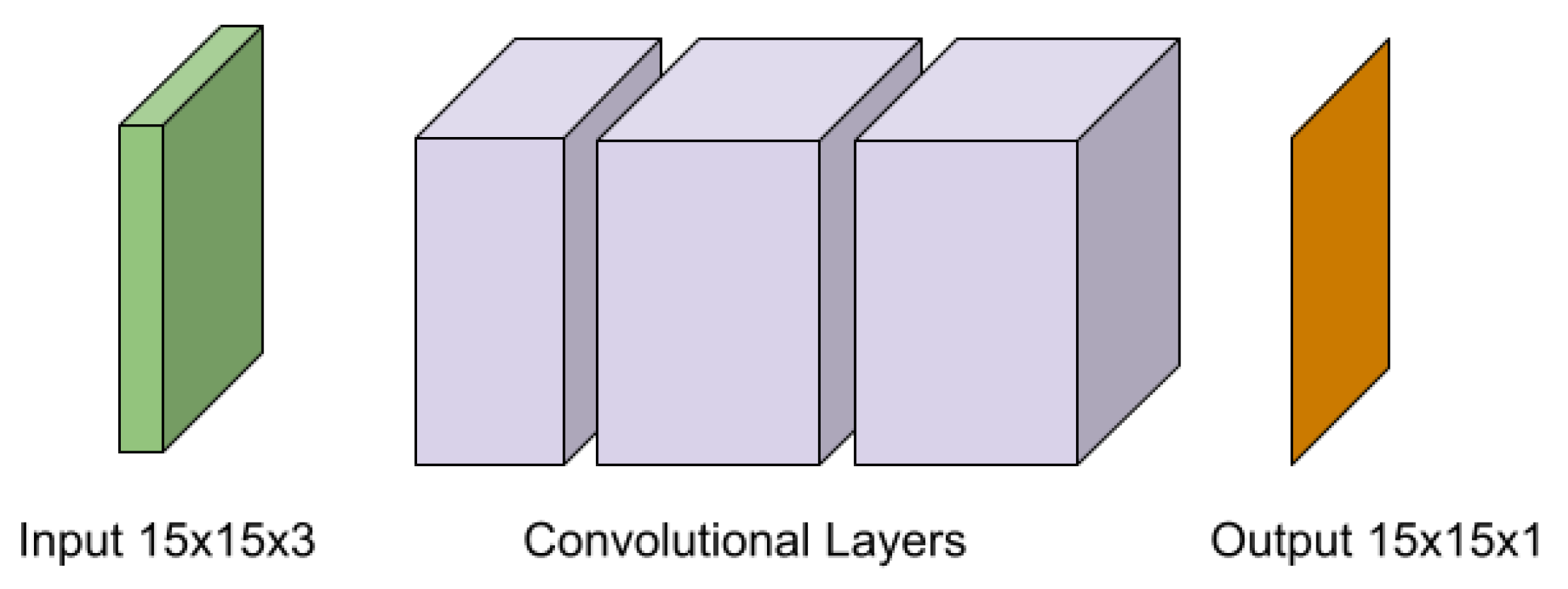
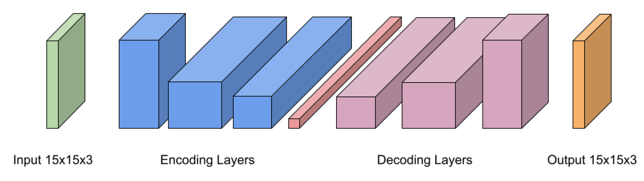
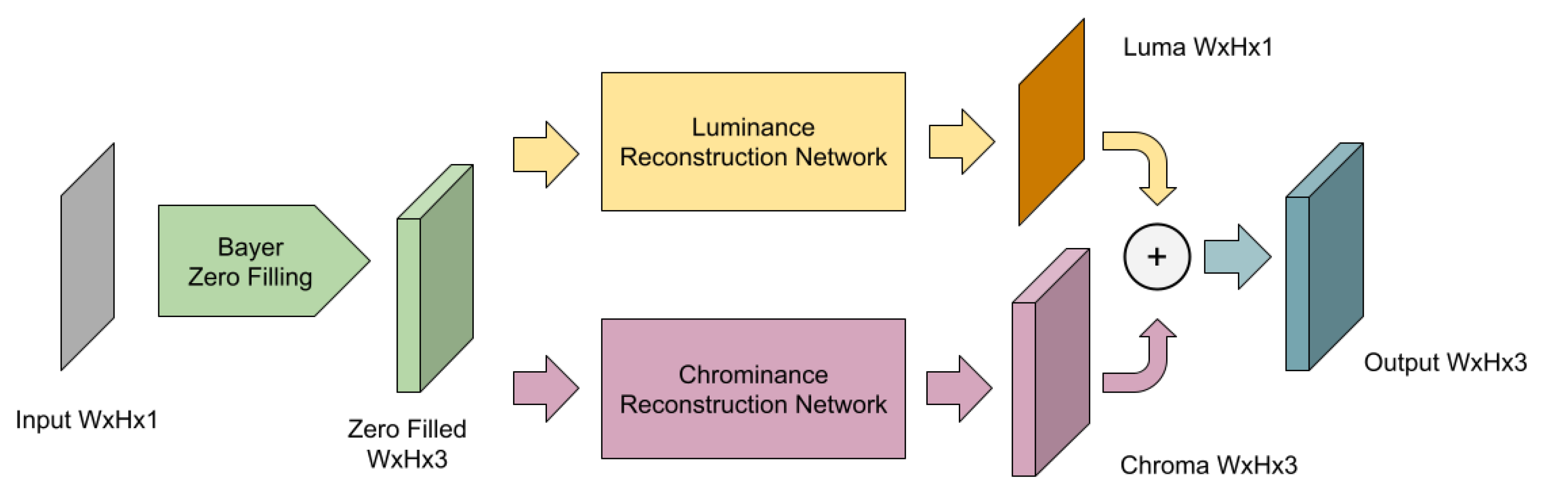
3.3. Convolutional Neural Network Model

Given that the Luminance and Chrominance estimations have different properties, we designed the full reconstruction network as two parallel networks: the Luminance reconstruction network and the Chrominance reconstruction network. These two networks are largely optimized for their specific task and can leverage a unique set of underlying modeling assumptions. The output of the two parallel networks are then combined in a final merging step to produce the final RGB output image.

3.4. Luminance Reconstruction Network

As observed in [19], the Luminance channels contain most of the high frequency components, thus the reconstruction algorithm should preserve such high frequency components. In [19], authors identify a specific 11 × 11 linear low-pass filter to estimate the image Luminance channel. We found, however, that the proposed filter produces blurred reconstructions. In order to improve the Luminance estimation, we suggest, as a slightly more complex filter, a nonlinear filter with learnable coefficients. We designed our Luminance estimation model as a three-layer neural network with sigmoidal activation functions. We compared models obtained using the mean squared error (l2-norm) and the maximum absolute error (l1-norm) as loss functions and found that sharper images can be obtained with the maximum absolute error.

The Luminance Reconstruction Network receives a 15 × 15 × 3 patch and outputs a 15 × 15 × 1 patch. Data is processed as a feed-forward network with a single internal hidden layer. In order to keep the implementation simple, we only used sigmoidal activation functions. The network is represented in Figure 7.

3.5. Chrominance Reconstruction Network

The reconstruction of the Chrominance vector has to be dealt with a different set of assumptions in mind. Specifically, as the Chrominance vector has mostly low-frequency components, blurred reconstructed images can still be valid estimations as they are compensated when combined with the Luminance channel in the final merging step. Therefore, the mean squared error can be used as an optimization function. Additionally, Chrominance channels have high inter-channel correlation, therefore it is possible that there exists an underlying nonlinear projection that is able to fully encode the correlations between channels. Based on these assumptions, we propose the Chrominance reconstruction model to be designed as a multi-layer encoder-decoder network.

The Chrominance Reconstruction Network is described in Figure 8. Similarly to the Luminance Reconstruction Networks, it receives a 15 × 15 × 3 patch and outputs a 15 × 15 × 3 patch. Internally, data is reduced to a lower-dimensional network by multiple layers of an Encoder Network and reconstructed by a Decoder Network to recover a full 15 × 15 × 3 image. We primarily used ReLU activation functions in hidden layers and a sigmoidal activation function for the output layer.

3.6. Full Reconstruction Network

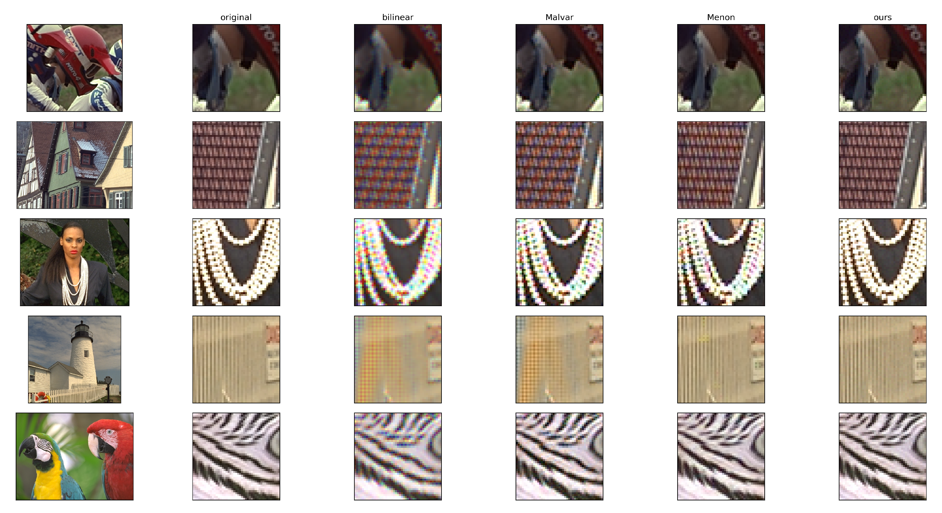
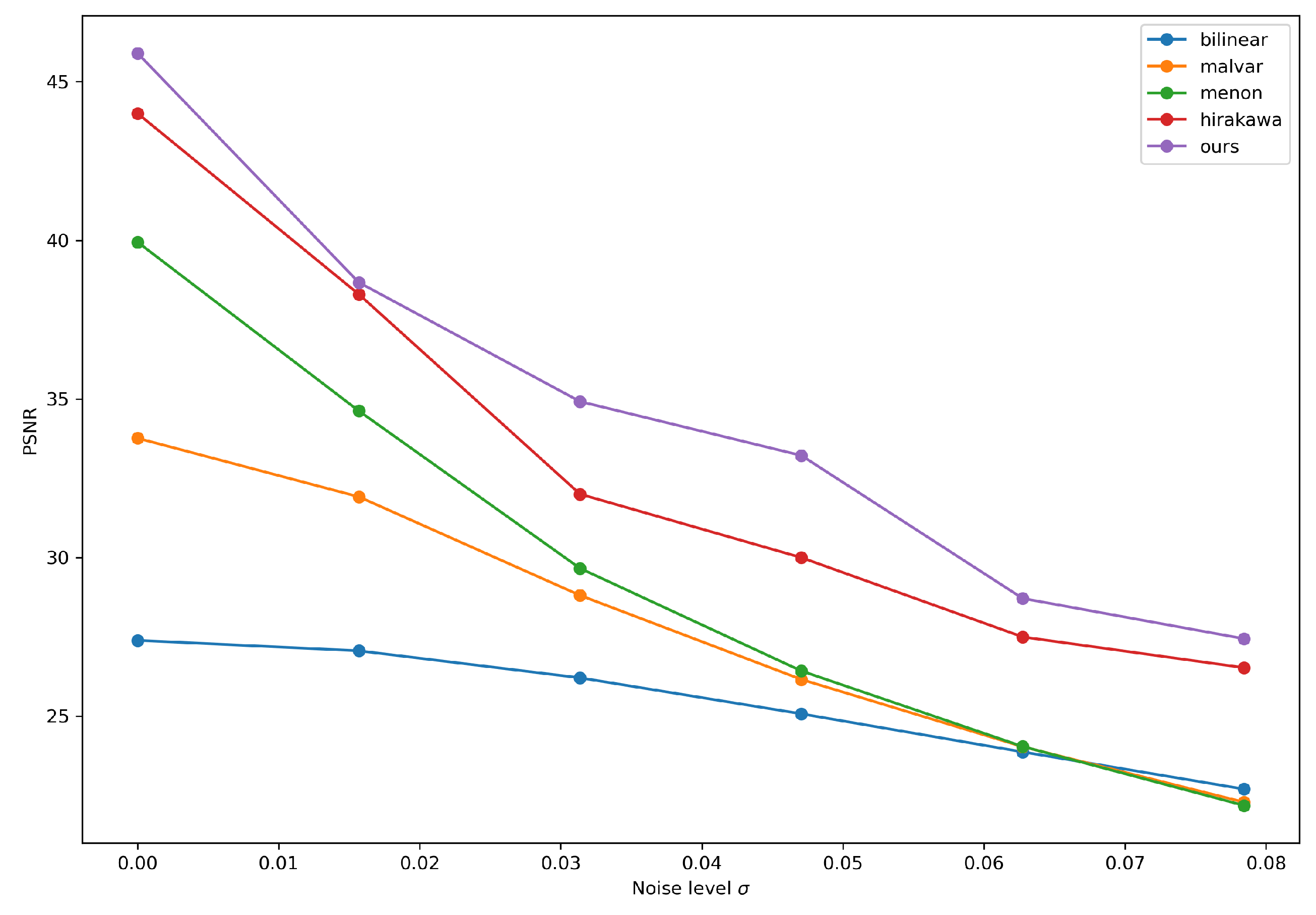
The Full Reconstruction network is a Fully Convolutional Neural Network that is a parallel composition of the two estimation networks for the Luminance and Chrominance channels. The network receives a 15 × 15 × 1 input patch as a Bayer patch and produces the estimated 16 × 16 × 3 RGB output patch. Since input Bayer patches have different configurations, the network converts the input 16 × 16 × 1 patch in three 15 × 15 patches, filling the unavailable color information with zeros. This approach has been proposed in [7] to simplify the alignment issues that arise from the possible Bayer configurations. The Full Reconstruction Network is responsible to keep track of the current configuration, and updates the patch conversion as it scans the overall image. This operation is graphically presented in Figure 9.

In the final merging step, the output RGB image is obtained from the two output results as a simple pixel-wise summation (see Equation (8)).

$$I_{est}(x,y)={\Phi }_{est}(x,y)+\left\{{\Psi }_{est}{(x,y)}_i\right\},i\in \{R,G,B\}$$

(8)

where ${\Phi }_{est}$ is the estimated Luminance channel and ${\Psi }_{est}$ is the estimated Chrominance three-dimensional vector.

The final model is represented Figure 10 with the output of its internal intermediate steps.

4. Results

In this section we compare our demosaicing algorithm to a selection of classical algorithms [14,24,25] and more recently developed techniques [7,20]. Among the large number of published work on demosaicing, we selected the ones that provide algorithm implementation or performance results. No general agreement exists on the kind of error function to be used when comparing the performance of demosaicing algorithms since perceived visual similarity between images is highly subjective. Nevertheless, different error functions have been defined to approximate the similarity between images as close as possible to human perception.

Distance-based functions have simple mathematical formulation and allow for a formal definition similarity between images, however they are often unable to discriminate images that contain visual artifacts. Examples of distance-based functions include Mean Squared Error, Mean Absolute Error, and Peak Signal-to-Noise Ratio (PSNR).

Distance-based functions can provide good approximation of the human perceived difference between two images if the image is first converted from RGB to CIE-lab color space. In CIE-lab color space, visually similar colors are also geometrically closer, thus chromatic differences between images can be compared. Specific quality functions such as the Structural Similarity Index (SSIM) can be used if better approximation of perceptual difference is required. Other functions specific for demosaicing are the blurring measurement, zipper effect measurement, false color measurement, subdetected/overdetected edges and shifted edges [8].

In this work we compared the performance of our algorithm using the MSE error function defined in CIE-lab color space, the PSNR function and the SSIM function. We computed the MSE in CIE-lab space using the formula in Equation (9).

$$MSE(I_{rgb},I_{est})=\frac{1}{3WH}∥rgb2lab(I_{rgb})-rgb2lab(I_{est})∥$$

(9)

where $I_{rgb}$ is the original RGB image, $I_{est}$ is the reconstructed image from the Bayer image, $∥·∥$ is the euclidean norm, $rgb2lab(·)$ is the color space conversion function between RGB and CIE-lab, W and H are the image width and image height.

The PSNR function is defined in Equation (10).

$$PSNR(I_{rgb},I_{est})=10lo{g}_{10}\left(\frac{max{(I_{rgb})}^2}{mse(I_{rgb},I_{est})}\right)$$

(10)

where $I_{rgb}$ is the original RGB image, $I_{est}$ is the reconstructed image from the Bayer image, and $mse(·)$ is the Mean Squared Error function. For the computation of the SSIM function we used its original definition, as provided in [26].

Similarly to other works in the literature [7,19,27], we used the Kodak dataset [6] as the benchmark dataset. The Kodak dataset is composed of 25 uncompressed PNG true color images of size 768 × 512 pixels. For testing the performance of different demosaicing algorithms, the dataset is usually divided into a training set of 10 images and a test set of 10 images. Images are subsampled using the Bayer pattern configuration and used as input to the demosaicing algorithm. The original RGB images are then compared to the demosaicing output using one of the previously described error functions [17,20,21]. In this work we follow the same overall procedure in order to compare as closely as possible our solution to existing algorithms. We note however that previous works do not report the registered quality metrics. When the algorithm implementation was available we computed the relative error function, but when no implementation was available we marked the entry as “not available”. We collected the results in

Table 1. Mean measured error performance in reconstruction for the entire Kodak dataset. For all three error functions we achieve the best performance when compared to other methods. (*) No implementation was available and only published results are reported.

	MSE	PSNR	SSIM
bilinear	0.14	29.2	0.93
Malvar [24]	0.07	35.4	0.98
Menon [25]	0.05	39.2	0.99
Hirakawa [14] *	-	36.5	-
Zhang [17] *	-	37.3	-
Heide [27] *	-	40.0	-
Jeon [28] *	-	36.4	-
Condat [29] *	-	35.5	-
Condat [30] *	-	36.1	-
ours	0.04	43.1	0.99

. Visual comparison is provided in Figure 11.

We analyzed the effect of both signal noise and quantization noise and compared the performance of our algorithm in both scenarios. The proposed model has a minimal performance drop due to signal noise and it is robust to quantization noise. Further improvement in robustness to signal noise can be achieved if the training set contains input samples corrupted by noise. To estimate image robustness to signal noise, we generated a number of samples corrupted by Gaussian random noise with varying intensity in order to simulate electrical noise captured by the camera sensor. We trained two models on the original training dataset and on a training dataset that included corrupted samples and compared the output produced by the two models after training. We reported results in Figure 12.

We measured filter coefficient quantization by applying post-train quantization on the resulting model. We compared the original floating point implementation to the model after coefficient quantization on 8-bit and measured the reconstruction error relative to the original input image. From the measurements we collected, the effect of quantization in this model is negligible and this enables the implementation of low-end devices that do not support floating-point units (FPGAs, low-end processors).

To test the performance on a real-world application, we implemented our model in NVIDIA CUDA on Jetson Nano on-board GPU and measured its performance over 1024 runs. We measured an end-to-end running for full frame high-resolution 12 MPixel image (4000 × 3000) of $996.22\pm 24.978$ ms.

5. Conclusions

In this work, we presented a novel data-driven demoisaicing algorithm that converts a raw image with Bayer pattern in an estimated RGB image. We observed the difference in the requirements for the Luminance estimation and the estimation of the three Chrominance channels and developed two reconstruction models. The two reconstruction models are integrated in a Full Reconstruction Network designed as a parallel composition of the two with a final merging step to recreate the output RGB image. In order to learn the input/output relations between the Bayer patches and the Luminance and Chrominance patches, we created a large dataset of patches extracted from the popular Kodak dataset. Additionally, we described the data selection strategy we followed to capture different populations of image patches with varying chromatic and spatial characteristics as an attempt to reduce model overfitting. We validated our result on a separate set of images and reported various reconstruction quality metrics. For the purpose of estimating the real applicability of the model and computational complexity, we deployed the proposed Full Reconstruction Network on the low-cost embedded system NVIDIA Jetson Nano.

6. Future Works

In future works we plan to compare our model to Generative Adversarial Networks (GANs) or Super-resolutions techniques. In this work we measured the effect of post-train quantization, however information about the quantization process can be included in the model to further improve its performance. Finally, we deployed our model on a embdedded GPU, but it may be feasible to implement the same model on FPGA to achieve higher data throughput.

References

1. Bayer, B.E. Color Imaging Array. 1976. Available online: http://www.google.com/patents?id=Q_o7AAAAEBAJ&dq=3,971,065 (accessed on 19 June 2021).
2. Lukac, R.; Plataniotis, K.N.; Hatzinakos, D.; Aleksic, M. A new CFA interpolation framework. Signal Process. 2006, 86, 1559–1579. [Google Scholar] [CrossRef] [Green Version]
3. Condat, L. A new random color filter array with good spectral properties. In Proceedings of the 2009 16th IEEE International Conference on Image Processing (ICIP), Cairo, Egypt, 7–10 November 2009; pp. 1613–1616. [Google Scholar]
4. Zapryanov, G.; Nikolova, I. Demosaicing methods for pseudo-random Bayer color filter array. In Proc. ProRisc; ProRisc: Veldhoven, The Netherlands, 2005; pp. 687–692. [Google Scholar]
5. Kröger, R.H. Anti-aliasing in image recording and display hardware: Lessons from nature. J. Opt. A Pure Appl. Opt. 2004, 6, 743. [Google Scholar] [CrossRef]
6. Kodak PhotoCD. Available online: https://www.math.purdue.edu/~lucier/PHOTO_CD/ (accessed on 5 September 2021).
7. Gharbi, M.; Chaurasia, G.; Paris, S.; Durand, F. Deep joint demosaicking and denoising. ACM Trans. Graph. (ToG) 2016, 35, 1–12. [Google Scholar] [CrossRef]
8. Losson, O.; Macaire, L.; Yang, Y. Chapter 5—Comparison of Color Demosaicing Methods. In Advances in Imaging and Electron Physics; Hawkes, P.W., Ed.; Elsevier: Amsterdam, The Netherlands, 2010; Volume 162, pp. 173–265. [Google Scholar] [CrossRef] [Green Version]
9. Gunturk, B.K.; Glotzbach, J.; Altunbasak, Y.; Schafer, R.W.; Mersereau, R.M. Demosaicking: Color filter array interpolation. IEEE Signal Process. Mag. 2005, 22, 44–54. [Google Scholar] [CrossRef]
10. Cok, D.R. Reconstruction of CCD images using template matching. In Proc IS&T Annual Conf./ICPS; St. Petersburg, Russia, 1994; pp. 380–385. [Google Scholar]
11. Hibbard, R.H. Apparatus and Method for Adaptively Interpolating a Full Color Image Utilizing Luminance Gradients. U.S. Patent No. 5,382,976, 17 January 1995. [Google Scholar]
12. Li, J.S.J.; Randhawa, S. High Order Extrapolation Using Taylor Series for Color Filter Array Demosaicing. In Image Analysis and Recognition; Kamel, M., Campilho, A., Eds.; Springer: Berlin/Heidelberg, Germany, 2005; pp. 703–711. [Google Scholar]
13. Hamilton, J.F.; Adams, J.E. Adaptive Color Plan Interpolation in Single Sensor Color Electronic Camera. U.S. Patent No. 5,629,734, 13 May 1997. [Google Scholar]
14. Hirakawa, K.; Parks, T. Adaptive homogeneity-directed demosaicing algorithm. IEEE Trans. Image Process. 2005, 14, 360–369. [Google Scholar] [CrossRef] [PubMed]
15. Chang, L.; Tan, Y.P. Hybrid color filter array demosaicking for effective artifact suppression. J. Electron. Imaging 2006, 15, 013003. [Google Scholar] [CrossRef]
16. Kimmel, R. Demosaicing: Image reconstruction from color CCD samples. IEEE Trans. Image Process. 1999, 8, 1221–1228. [Google Scholar] [CrossRef] [PubMed] [Green Version]
17. Zhang, L.; Wu, X.; Buades, A.; Li, X. Color demosaicking by local directional interpolation and nonlocal adaptive thresholding. J. Electron. Imaging 2011, 20, 023016. [Google Scholar]
18. Wang, C. Bayer patterned image compression based on wavelet transform and all phase interpolation. In Proceedings of the 2012 IEEE 11th International Conference on Signal Processing, Beijing, China, 21 October 2012; Volume 1, pp. 708–711. [Google Scholar]
19. Alleysson, D.; Susstrunk, S.; Hérault, J. Linear demosaicing inspired by the human visual system. IEEE Trans. Image Process. 2005, 14, 439–449. [Google Scholar] [PubMed] [Green Version]
20. Syu, N.S.; Chen, Y.S.; Chuang, Y.Y. Learning deep convolutional networks for demosaicing. arXiv 2018, arXiv:1802.03769. [Google Scholar]
21. Tan, R.; Zhang, K.; Zuo, W.; Zhang, L. Color image demosaicking via deep residual learning. In Proceedings of the IEEE Int. Conf. Multimedia and Expo (ICME), Hong Kong, China, 10–14 July 2017; Volume 2, p. 6. [Google Scholar]
22. Gunturk, B.K.; Altunbasak, Y.; Mersereau, R.M. Color plane interpolation using alternating projections. IEEE Trans. Image Process. 2002, 11, 997–1013. [Google Scholar] [CrossRef] [PubMed]
23. Khashabi, D.; Nowozin, S.; Jancsary, J.; Fitzgibbon, A.W. Joint Demosaicing and Denoising via Learned Nonparametric Random Fields. IEEE Trans. Image Process. 2014, 23, 4968–4981. [Google Scholar] [CrossRef] [PubMed]
24. Getreuer, P. Malvar-He-Cutler Linear Image Demosaicking. Image Process. Line 2011, 1, 83–89. [Google Scholar] [CrossRef] [Green Version]
25. Menon, D.; Andriani, S.; Calvagno, G. Demosaicing with directional filtering and a posteriori decision. IEEE Trans. Image Process. 2006, 16, 132–141. [Google Scholar] [CrossRef] [PubMed]
26. Wang, Z.; Bovik, A.C.; Sheikh, H.R.; Simoncelli, E.P. Image quality assessment: From error visibility to structural similarity. IEEE Trans. Image Process. 2004, 13, 600–612. [Google Scholar] [CrossRef] [PubMed] [Green Version]
27. Heide, F.; Steinberger, M.; Tsai, Y.T.; Rouf, M.; Pająk, D.; Reddy, D.; Gallo, O.; Liu, J.; Heidrich, W.; Egiazarian, K.; et al. FlexISP: A Flexible Camera Image Processing Framework. ACM Trans. Graph. 2014, 33, 1–13. [Google Scholar] [CrossRef] [Green Version]
28. Jeon, G.; Dubois, E. Demosaicking of noisy Bayer-sampled color images with least-squares luma-chroma demultiplexing and noise level estimation. IEEE Trans. Image Process. 2012, 22, 146–156. [Google Scholar] [CrossRef] [PubMed]
29. Condat, L. A new color filter array with optimal properties for noiseless and noisy color image acquisition. IEEE Trans. Image Process. 2011, 20, 2200–2210. [Google Scholar] [CrossRef] [PubMed] [Green Version]
30. Condat, L.; Mosaddegh, S. Joint demosaicking and denoising by total variation minimization. In Proceedings of the 2012 19th IEEE International Conference on Image Processing, Orlando, FL, USA, 30 September–3 October 2013; pp. 2781–2784. [Google Scholar]
Figure 1. Example of a Bayer filter GRGB configuration. Input light source is filtered by the CFA before being acquired by the camera sensor. For each pixel in the CFA image, only one color is registered.
Applsci 11 09975 g001
Figure 2. Examples of typical demosaicing reconstruction artifacts for a sample image in Kodak dataset [6].
Applsci 11 09975 g002
Figure 3. Bayer configurations.
Applsci 11 09975 g003
Figure 4. Dataset creation process. From each input image, a collection of patches is extracted. For each patch a vector of feature is computed and used for clustering. A fixed number of patches is randomly sampled from each cluster to form the final collection of input/output pairs that are used as training and test samples.
Applsci 11 09975 g004
Figure 5. Examples of patches extracted from the Kodak dataset. Patches are automatically grouped by K-means clustering algorithm by chromatic and spectral similarity.
Applsci 11 09975 g005
Figure 6. Example of Fourier transform for input Bayer image from Kodak [6] dataset. In the Fourier transform diagram, the nine regions described in Equation (7) can be easily identified.
Applsci 11 09975 g006
Figure 7. Luminance Reconstruction Network.
Applsci 11 09975 g007
Figure 8. Chrominance Reconstruction Network.
Applsci 11 09975 g008
Figure 9. During the scanning of the whole input Bayer image, the network local receptive field corresponds to different Bayer configurations. This means that two input vectors may have values for two different color channels in the same positions. To solve this alignment issue, the network can internally convert the input vector in three 15 × 15 patches that are zero-filled when the relative color information is unavailable. The three converted patches are always aligned and can be processed by the two parallel networks. The Full Reconstruction Network is responsible to constantly keep track of the current scanning position and convert the input vector to the appropriate output based on the current Bayer configuration. To simplify readability, we depicted the conversion of a 3 × 3 input vector. The current implementation extends this idea to a 15 × 15 input vector, however the number of configurations encountered during the scanning process does not change.
Applsci 11 09975 g009
Figure 10. Structure of the Full Reconstruction Network. Input image is preprocessed by converting the Bayer CFA image to a zero-filled RGB image. The preprocessed image is fed to the Luminance Reconstruction Network and the Chrominance Reconstruction Network. The Luminance Reconstruction Network produces a single channel image, the Chrominance Reconstruction Network, a three-channel image. Both outputs are merged in the final output RGB image.
Applsci 11 09975 g010
Figure 11. Comparison of our approach with Bilinear, Malvar [24], Menon [25] on noise-free images.
Applsci 11 09975 g011
Figure 12. PSNR comparison joint denoising and demosaicking at different levels of Gaussian noise with standard deviation σ . Higher values of PSNR correspond to better reconstruction. Our model is able to cope with relatively high level of noise. In order to provide a fair comparison, we reported the performance scores obtained by a model trained on a noise-free dataset. Further robustness to noise is possible if the training dataset is augmented with samples corrupted by noise.
Applsci 11 09975 g012