Article

Improved Training of CAE-Based Defect Detectors Using Structural Noise

Faculty of Science and Engineering, Saga University, Saga 840-8502, Japan
*
Author to whom correspondence should be addressed.
Appl. Sci. 2021, 11(24), 12062; https://doi.org/10.3390/app112412062
Submission received: 9 November 2021 / Revised: 11 December 2021 / Accepted: 16 December 2021 / Published: 17 December 2021
(This article belongs to the Special Issue Advances in Digital Image Processing)

Abstract

:

Featured Application

Detection of defective items on a production line, using artificial intelligence applied to image processing.

Abstract

Appearances of products are important to companies as they reflect the quality of their manufacture to customers. Nowadays, visual inspection is conducted by human inspectors. This research attempts to automate this process using Convolutional AutoEncoders (CAE). Our models were trained using images of non-defective parts. Previous research on autoencoders has reported that the accuracy of image regeneration can be improved by adding noise to the training dataset, but no extensive analyse of the noise factor has been done. Therefore, our method compares the effects of two different noise patterns on the models efficiency: Gaussian noise and noise made of a known structure. The test datasets were comprised of “defective” parts. Over the experiments, it has mostly been observed that the precision of the CAE sharpened when using noisy data during the training phases. The best results were obtained with structural noise, made of defined shapes randomly corrupting training data. Furthermore, the models were able to process test data that had slightly different positions and rotations compared to the ones found in the training dataset. However, shortcomings appeared when “regular” spots (in the training data) and “defective” spots (in the test data) partially, or totally, overlapped.

1. Introduction

In order to earn the trust of their customers, striving to offer the highest product quality is crucial for manufacturers. The foremost evidence of this quality to customers is: their appearances. Commercialization of faulty items can be prevented thanks to visual inspection: technicians removing defective parts from the line. The expertise and knowledge of these workers allow them to detect slight imperfections on products. Their ability to detect defects is the result of their experience, therefore it is difficult to hand it down to new colleagues, as every individual has their subjective judgments. Even though humans can adapt, their perception can be altered by their physical and environmental conditions. Finally, every operator is not necessarily reliable, as falsification of inspection records has been a growing problem. Modern industry revolves around technological innovations such as robots and Artificial Intelligence (AI), with computer-operated machines gradually replacing humans for the execution of laborious tasks. So far, even though improvements in the field of “visual inspection” are studied [1], its automation remains rather problematic. The advent of AI made the transition feasible. In this respect, this study intended to design a novel defect detection method analyzing the effect of noisy training on CAEs.
Computer vision research applied to image processing has evolved significantly in recent years [2]. Through their experimentations, researchers have proposed and developed numerous autonomous visual inspection systems. There are several techniques to inspect a picture, from a simple sorting of its pixels’ values via an intensity histogram to progressive indexes such as texture information or High-order Local AutoCorrelation (HLAC) [3], to mention a few. The typical process, old-fashioned and specific, is to create a reference image that represents the “average” appearance of flawless products [4]. This reference is then used to detect the defects on other images, comparing the values of their respective pixels: if targets contain patterns that are not on the “reference image”, they are considered defective. Even though this technique can be applied to a wide range of products, when no reference is available, generating such an image takes time and requires a lot of samples. Feature extraction is a more modern procedure for analyzing images [5], while being resilient to the variations in the data. Features are sets of data contributing to the categorization of their targets. A few common feature extraction approaches are template matching, deformable template, and graph description. Features extraction algorithms are often used in conjunction with classifiers, so targets can be detected (thanks to the extraction of their features) and categorized (thanks to classifications of the features extracted). The more relevant to the categories they are extracted from, the more useful these features are for classification. There are various classifiers available now such as decision trees [6] and Support Vector Machines (SVMs) [7]. Deep learning and end-to-end solutions have tended to grow in popularity as classifiers because they are able to learn features automatically. In the case of our study, instead of comparing two pictures, one picture is “scanned” by several filters to reveal “features” that may be categorized as “flaws”. These filters initially take time to be adjusted, but they virtually work on any image input. When a filter has located and extracted a feature, it is processed by a classifier that labels it as either “defective” or “normal”. If one, or more, features are labeled “defective”, then the whole part is regarded as “defective”.
Shortcomings remain in both “traditional” and “feature extraction—classification” methods. In the “traditional” method, the detection accuracy heavily relies on the shape, location, and orientation of the targets. Therefore, a complex structure, a slightly unusual outline or even an uncommon position, may lead to poor results. As for the “feature extraction—classification” method, trainings of models require a lot of samples, while some crucial data may be difficult to collect (such as gathering abnormal data). This problem is mitigated in our method as training the Neural Networks (NNs) requires unimpaired data, which are plentiful. Finally, some previous studies also focused on the use of autoencoders to restore altered pictures, while some others studied the influence of noise on neural networks. Indeed, it has been proven that noise injection (adding noise during their training phase) enhances the “generalization ability” of neural networks, i.e., their aptitude to apply operations they learned from known data to new sets of data. However, unlike our approach, they did not analyze the effects on the restoration ability of CAEs when different noise components were added to the input data, they rather observed the effects of noise injected to the input and output of the hidden layers. In this research, in an attempt to increase their accuracy, the use of autoencoders as anomaly detectors [8] was re-explored through the involvement of structural noise during their training phases.

2. Contrasts between the Classic Usage of Autoencoders and Ours

This section will briefly introduce autoencoders and our novel approach.

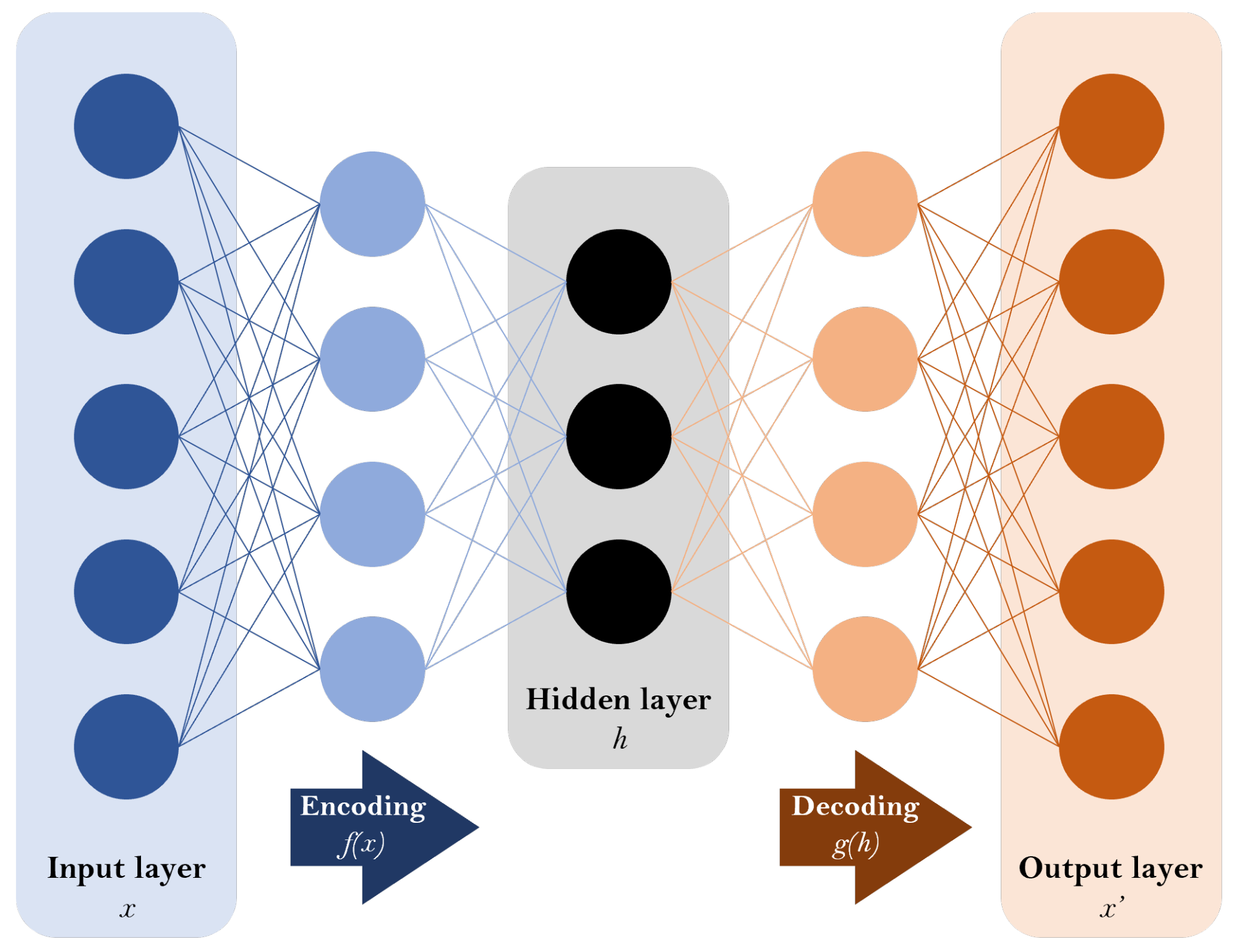
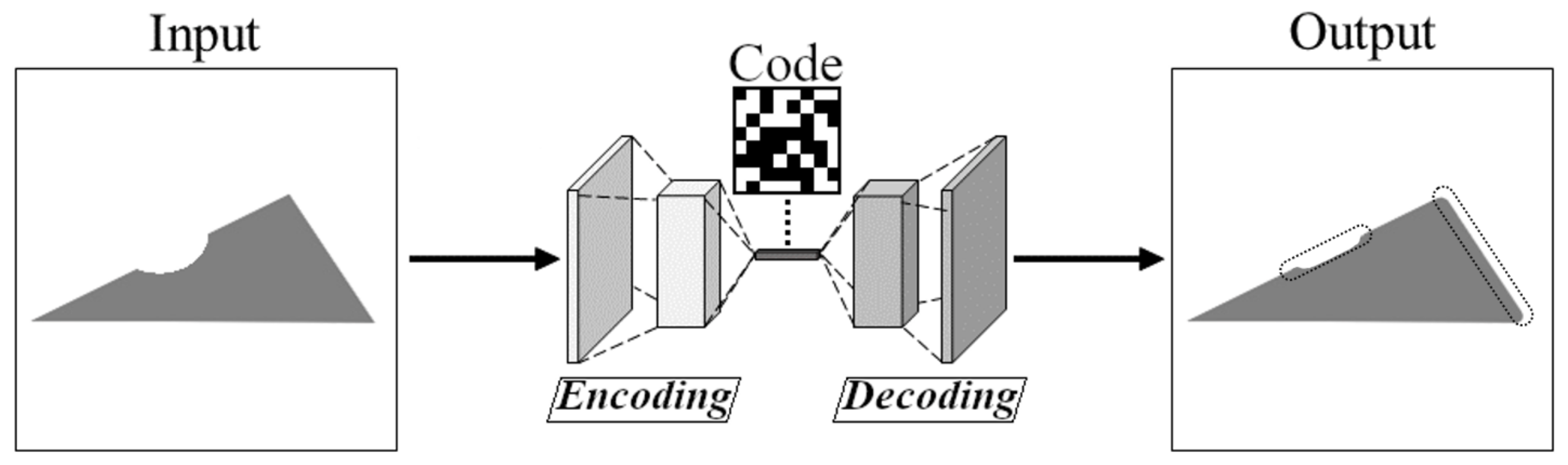
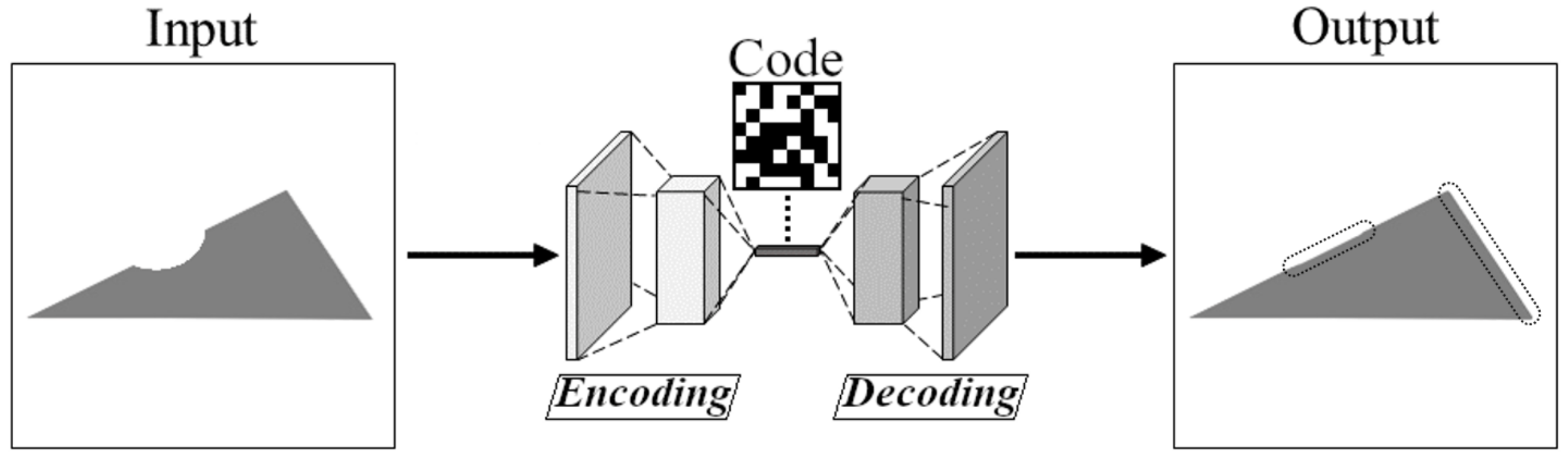
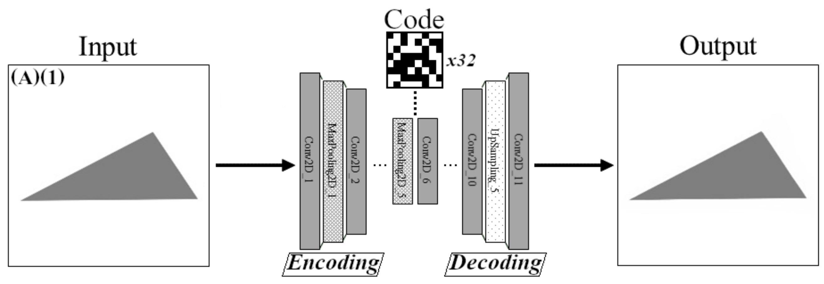
2.1. Working Principle of Autoencoders

Autoencoders are NN models trained through unsupervised learning algorithms. A simple structure of an autoencoder is shown in Figure 1.
A CAE takes data x as inputs, encodes f ( x ) them into “compressed” formats h (dimensionality reduction in the latent space as “codes”), and then decodes g ( h ) them into “uncompressed” data x (restored dimensionality), with as little losses as possible. The circles and lines in Figure 1 correspond to neurons and weights, which mimic the operations of biological synapses. The outputs of one layer of neurons are weighted by their respective coefficients and are transferred to the next layer of neurons. As no labeled datum is involved during its training phase, an autoencoder is said to be an unsupervised NN. More specifically, as input data are the only references to adjust its weights, it is said to be a “self-supervised NN”. After that a datum has been processed by the autoencoder, an energy function computes the differences between its uncompressed and its original forms. Then, in order to decrease the errors, these differences are exploited to fine-tune the weights within the NN. Therefore, a CAE attempts to learn efficient data encoding from successive compressions/decompressions: “compressions” are kinds of feature extractions from the data, whereas “decompressions” are reconstructions of the data from the features extracted.

2.2. Alternative Use of Autoencoders in Our Research

Our study re-explored autoencoders used to restore altered pictures [9,10,11], but, the restored pictures are then used to detect the alterations that were present within the original images. These networks are trained on flawless images and are able to reconstruct defective images that are input during the test phase. The encoder adjusts its weights to reduce data effectively, while the decoder adjusts its to restore encoded data as closely as possible to their original versions. As the autoencoder will have been accustomed to process pictures that are not defective, it will not treat faulty ones differently and will try to reform them as if they were flawless. The output will be an approximation of the unimpaired version of the flawed part, because the encoder is fit to regular data and codes anything as such, while the decoder handles the seemingly “flawless” encoded data normally. In this way, the differences between the input and the output can be counted as irregularities.
As shown in Figure 2, the architecture of our CAE is divided into two sequences of layers: convolutional and max pooling layers for the encoding, convolutional and upsampling layers for the decoding.
Since defective data are uncommon, being able to prepare these NNs from regular data is an advantage: it is laborious to form proper/relevant training datasets from scarce resources. In addition, it is known that the reduction/restoration ability of convolutional autoencoders is improved by the addition of noise to the input layer and the hidden layer [12,13]. Therefore, our study intended to determine what kind of noise should be used to get the best performances. Experiments involving no noise, Gaussian noise and a noise made of a known structure were conducted.
The Figure 3 presents typical flawed pieces and their flawless counterparts. These pictures are for illustration purposes; no actual restoration was performed, these are results sought in our study.

3. Improvement of Defect Detection Accuracy Using Structural Noise

This part is about the process behind defect detection and the training of neural network models with noisy images.

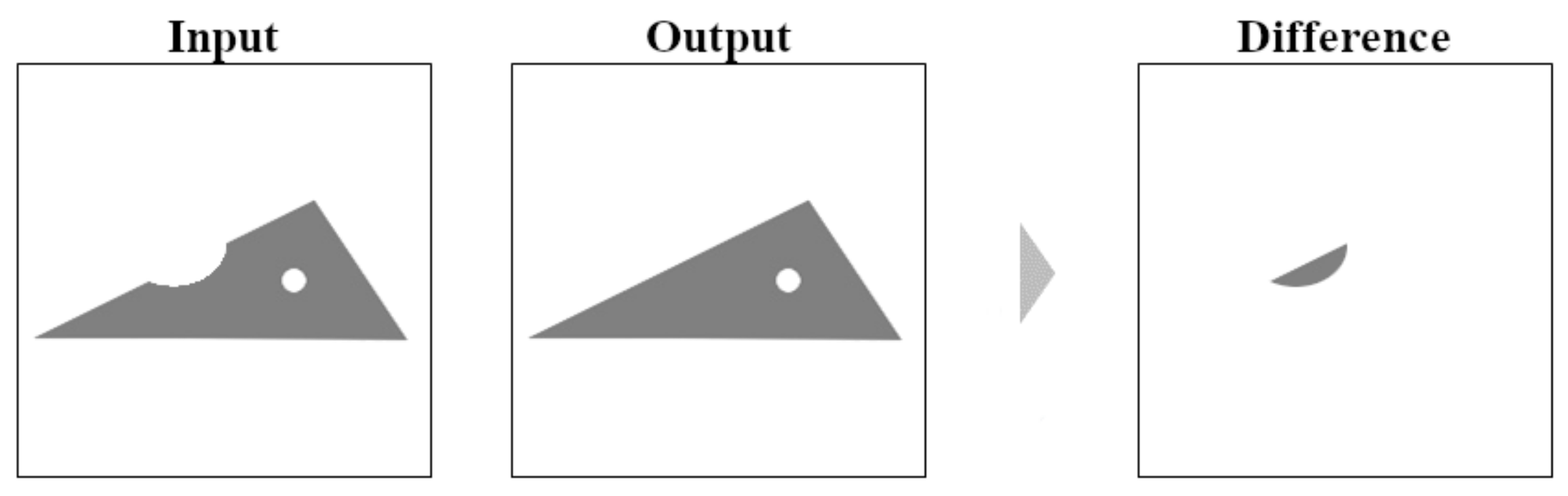
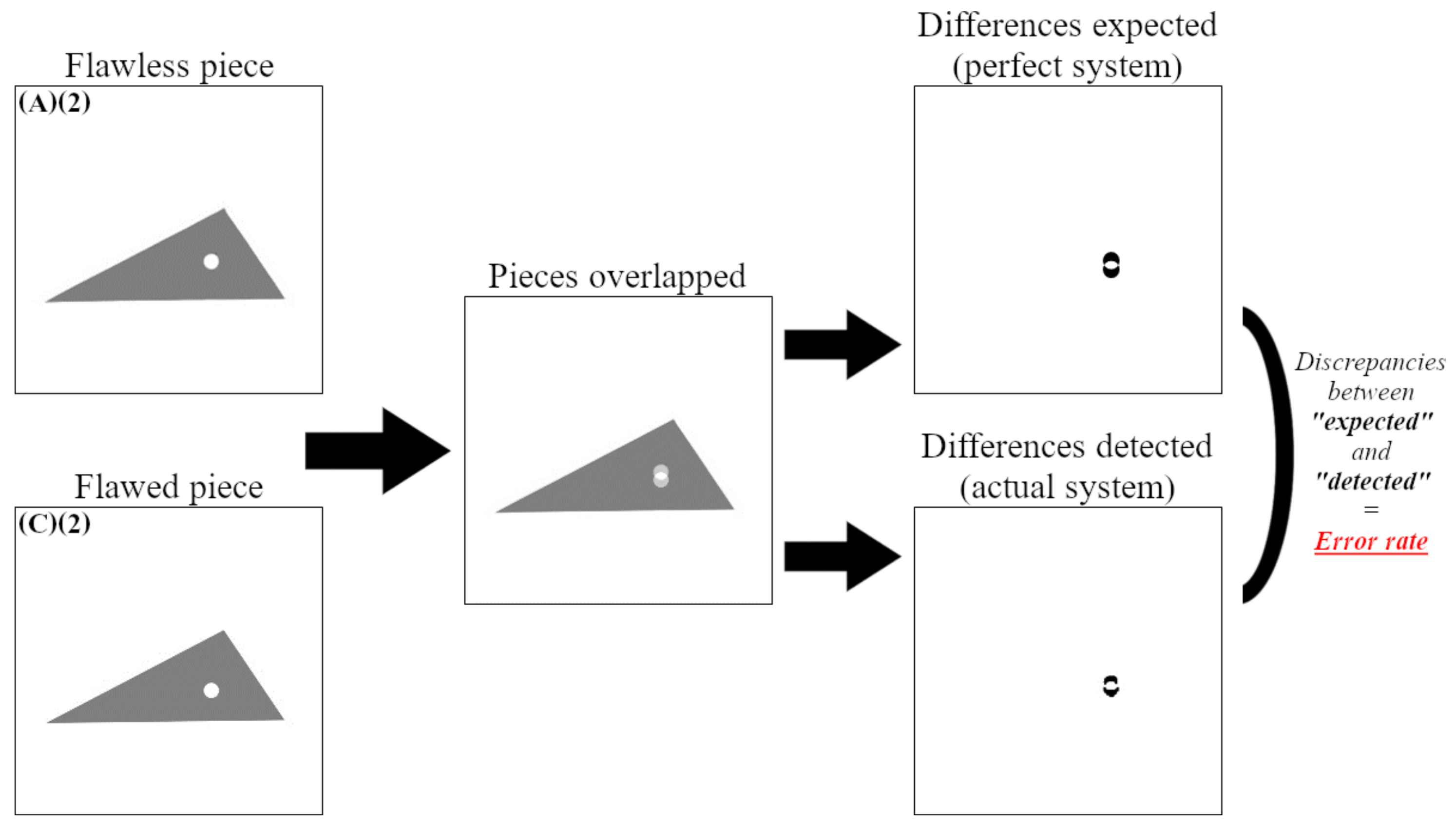
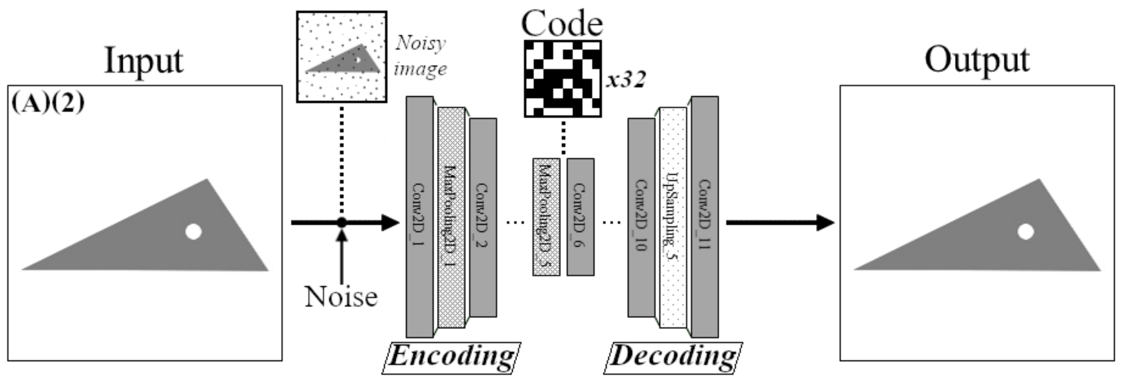
3.1. Defect Detection Using CAEs

As introduced in the previous section, a CAE is first trained on a dataset made of pictures of flawless pieces. Once ready, this model is fed defective images of which it must spot irregularities. Once the reconstruction is done, the areas that differ between the input and the output are considered “defective”, as in Figure 4 (where the output is shown as perfect for explanation purposes).
As the neural network is trained on pieces that are intact, it does not know how to handle a faulty piece, thus, it attempts to encode and decode it as a regular piece. Since the faulty pieces are processed indifferently, the “code” is decoded as usual, which leads to output an approximation of what the piece would look like without flaws. For example, in Figure 5, an image of a damaged piece is fed to an autoencoder.
It should be noted that this works only for the defective pieces of which similar counterparts were used to train the model. If the shapes, sizes, positions or rotations of the pieces tested contrast too much with those of training data, the model will not be able to handle them correctly. Adding noise to the training dataset can improve the reconstruction phase. In this way, the autoencoders become more resilient to slight variations in the data they handle.

3.2. Network Training with Noisy Data

Noisy training of autoencoder is known to benefit its models [12,13,14]. Noise injection [15,16] or slight corruption of its inputs [17,18] can improve its generalization ability: its aptitude to apply the operations it learned from known data to new sets of data. The noise acts like some sort of data augmentation, which prevents the network from overfitting on the training dataset. The encoding/decoding capability of the autoencoders can also benefit from this, by noising the values processed in the input and hidden layers, as shown in Figure 6.
CAEs are trained by lowering the values returned by their energy functions as much as possible, as these values indicate the error between the reconstructed images and their “teacher data” (their original forms). Therefore, if noise is added to the images before that they are input to the CAE, the reconstructed data can be compared to the noiseless data, which will exercise the network to denoise noisy pictures. However, the output is never perfect: some loss is always induced because of the compression/decompression processes.

4. Experiments

This section details the experiments conducted to evaluate the usefulness of the proposed defect detection method. They were carried out on a workstation operating on Ubuntu 18.04.3 LTS and built from the following hardware: Intel Core i7-8700 CPU, Nvidia TITAN V/PCie/SSE2 GPU, 32 Gb RAM memory. It is important to note that the data of the study did not involve actual pieces but simple triangular shapes. This choice was made to simulate pieces with different positions, rotations and defects.

4.1. Experimental Settings

Custom datasets were generated for the experiments to use data of which content is controlled and known. This helped draw conclusions from the observations made when noise injections were added through the study.

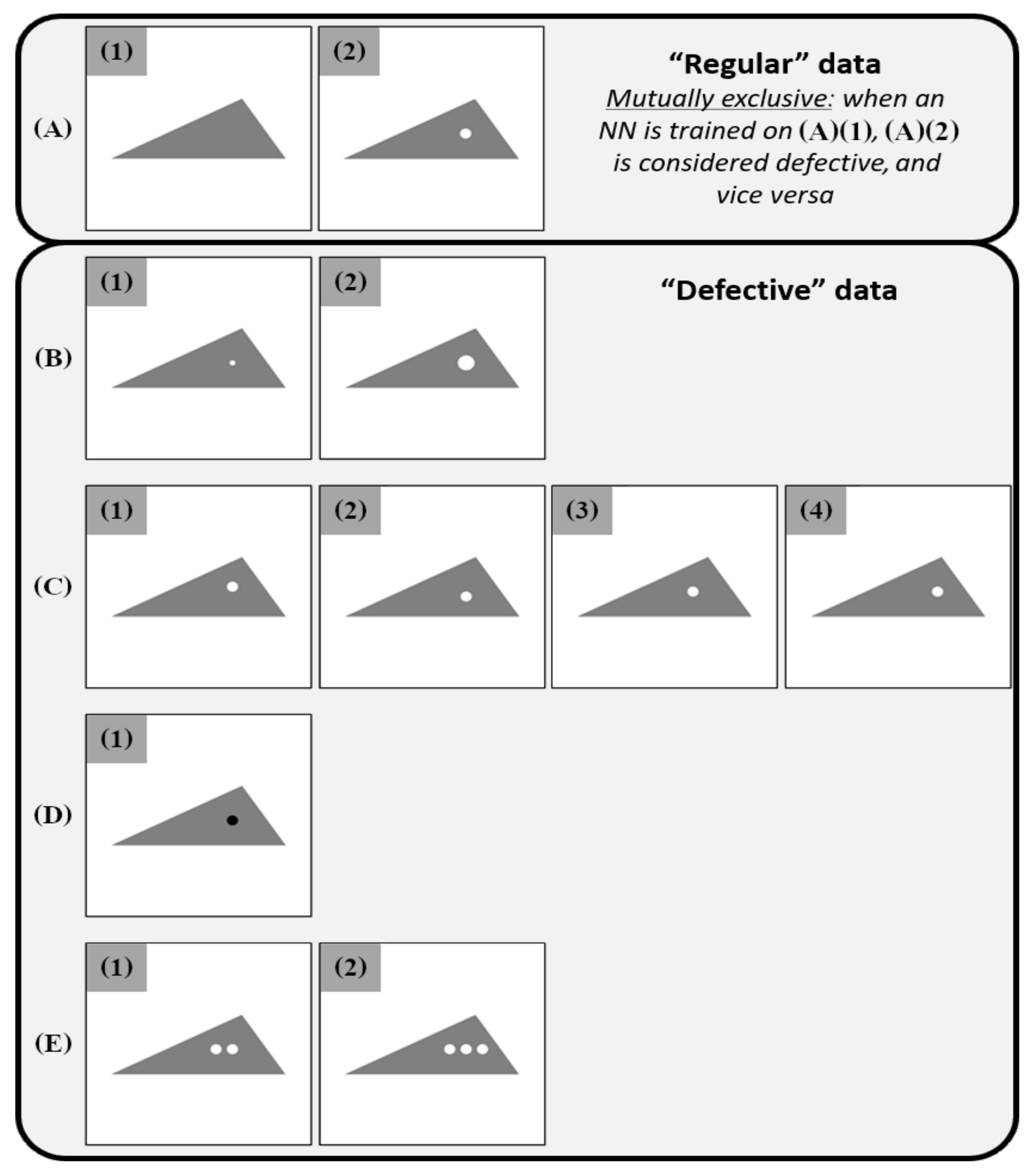
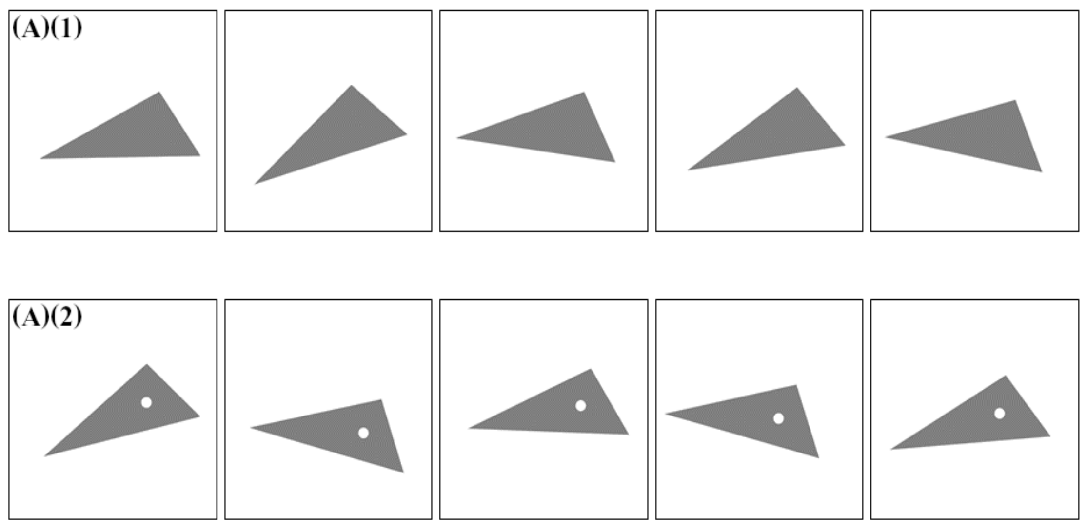
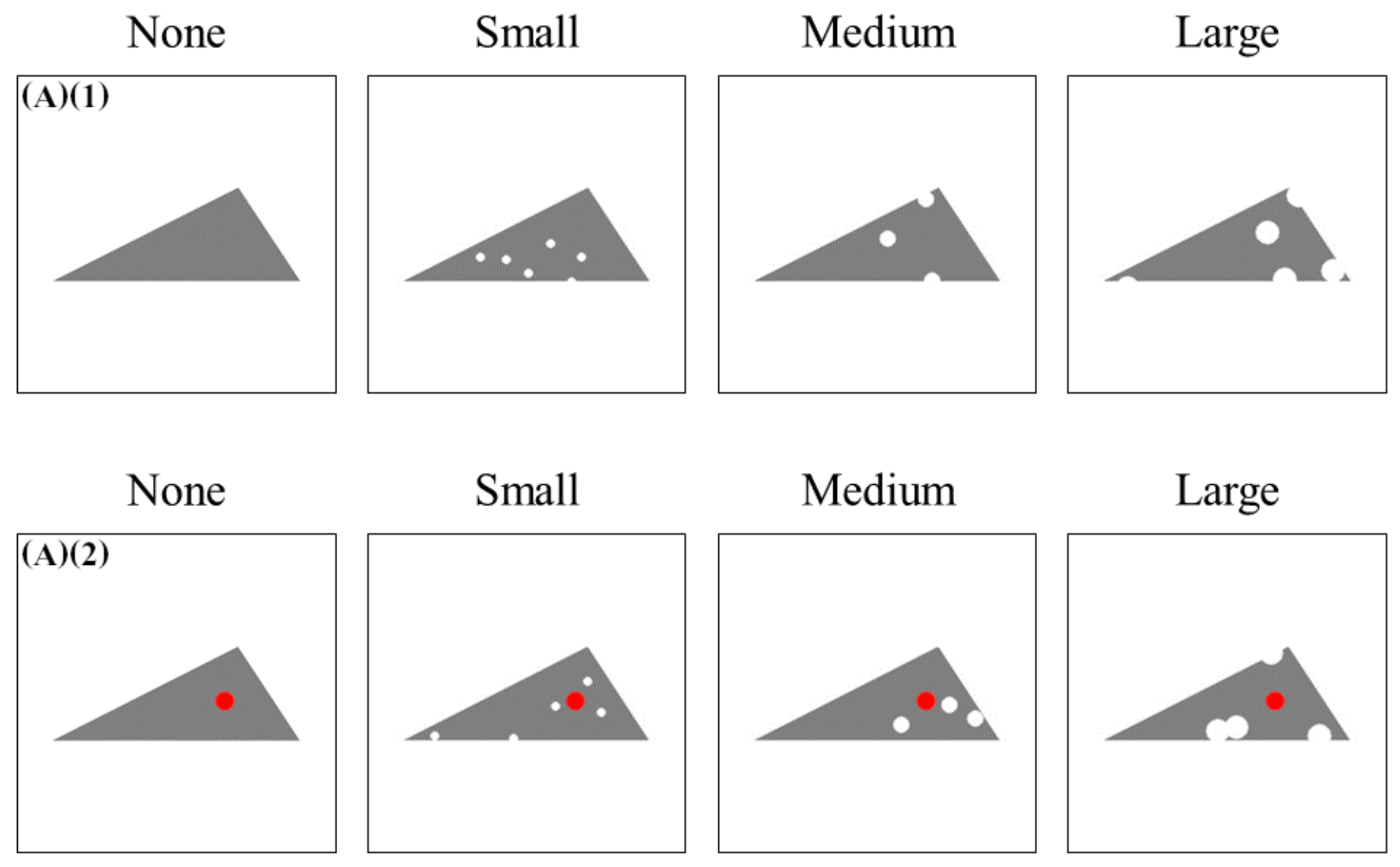
4.1.1. Compositions of the Training/Test Datasets

The sets of images we used were artificially generated with a drawing software. They are grayscale pictures of which dimensions are 256 × 256 px with a resolution of 72 dpi. Originally, the values of the pixels ranged from 0 to 255, but they were normalized to range from 0 to 1. One triangle about 199 px wide and 75 px tall is drawn within each picture. Although detailed analysis were not performed, simple preliminary experiments were conducted on quadrilaterals and circles and resulted in observations similar to that of triangles. The breakdown of the dataset is shown in the Table 1, which shows the five categories and their variations.
Two categories are considered “regular”: spotless triangles (A)(1) and spotted triangles (A)(2). However, only one at a time can be used during the training phase of a model, the other is then considered “defective” during its testing phase. Additionally, some datasets ((B), (C), (D), (E)) are “defective”, regardless of the data used to train the model and are always used for testing purposes. They are made of spotted triangles whose spots are generated depending on several parameters, such as: their size (B), position (C), color (D) and count (E), which result into 9 defect patterns. Only a few defects were simulated, as there are a lot of parameters to take into consideration, we had to narrow down our attention and decided to examine a limited number of flaws characterized by one abnormal parameter at a time, instead of combinations. Some examples are displayed in Figure 7.
In real life conditions, during their inspection, the pieces are everywhere but rarely centred within the camera’s field of vision. To simulate these misalignments, the triangles also underwent translations and rotations from time to time, as shown in Figure 8.
For our experiments, two pairs of training/test datasets were formed:
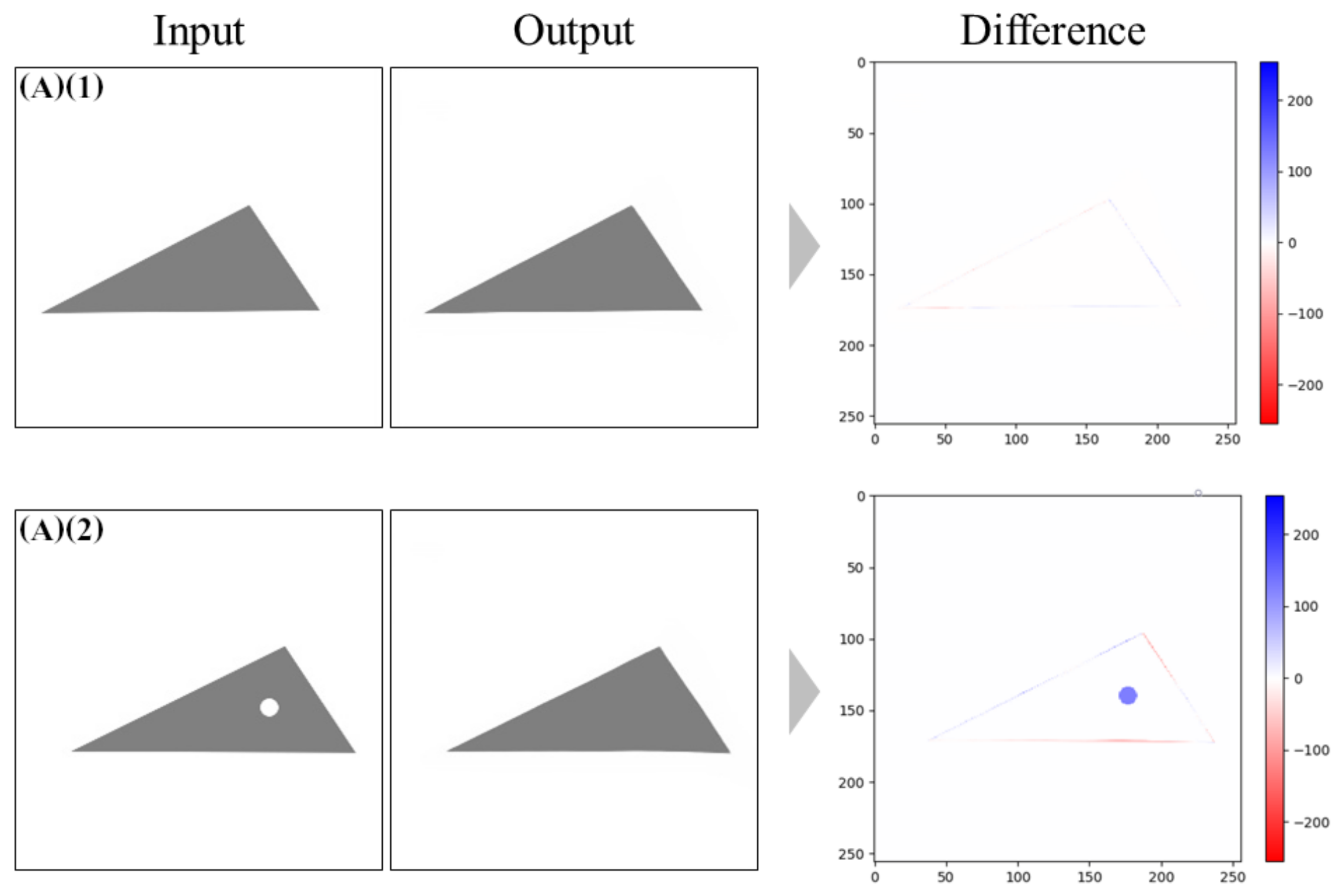
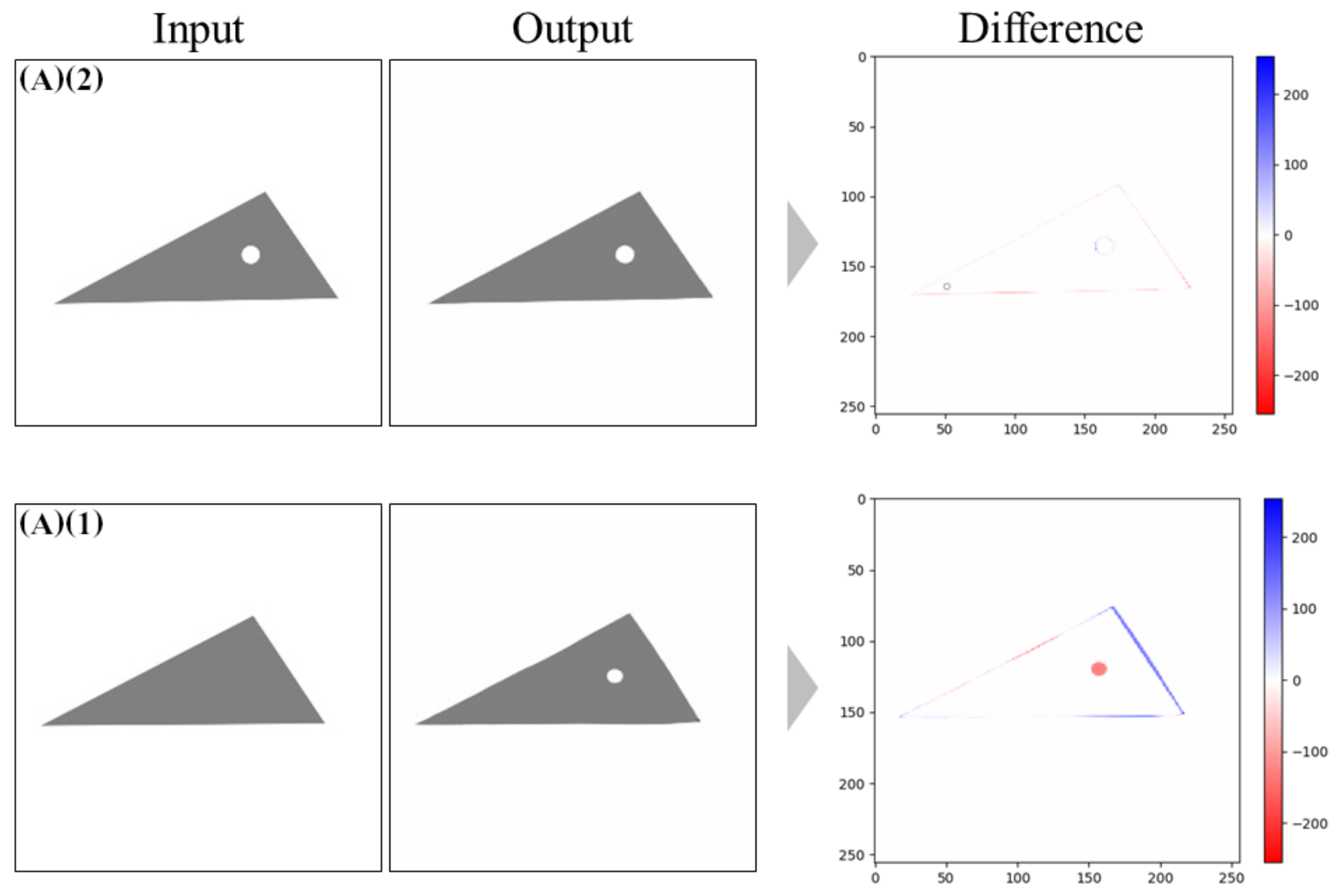
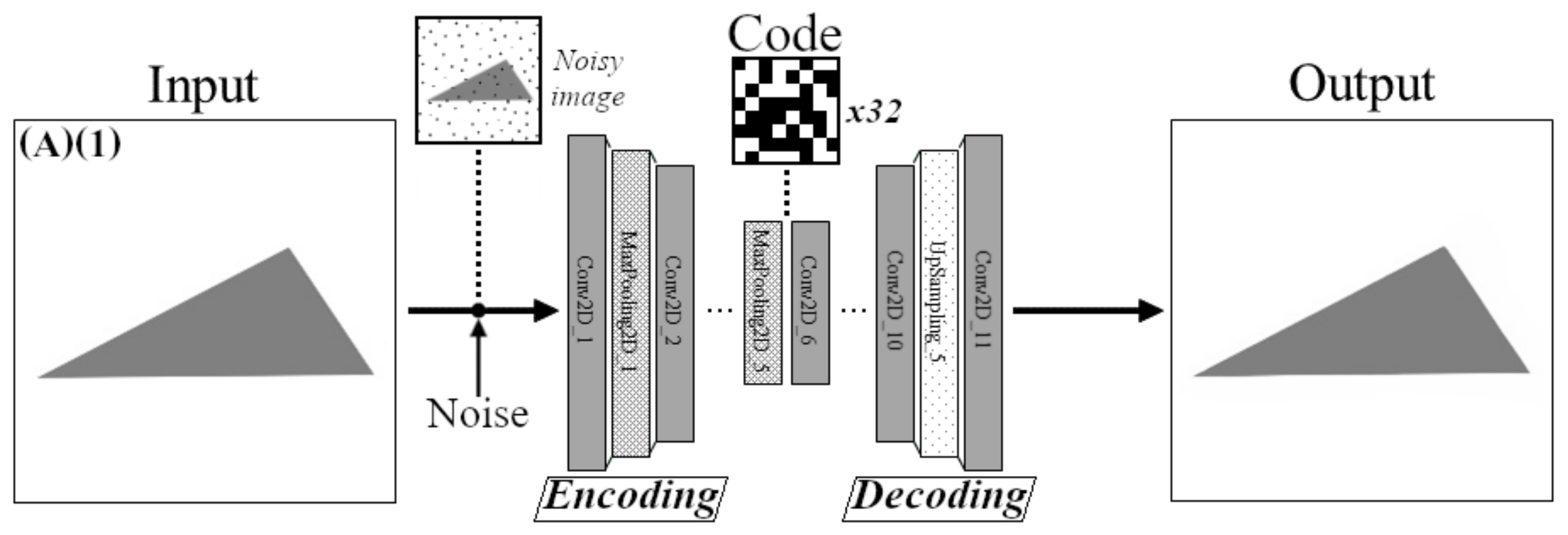
  • a training dataset made of 800 regular spotless triangles (A)(1) and a test dataset mixing 2000 defective samples (200 of each other class in the Table 1, including (A)(2))
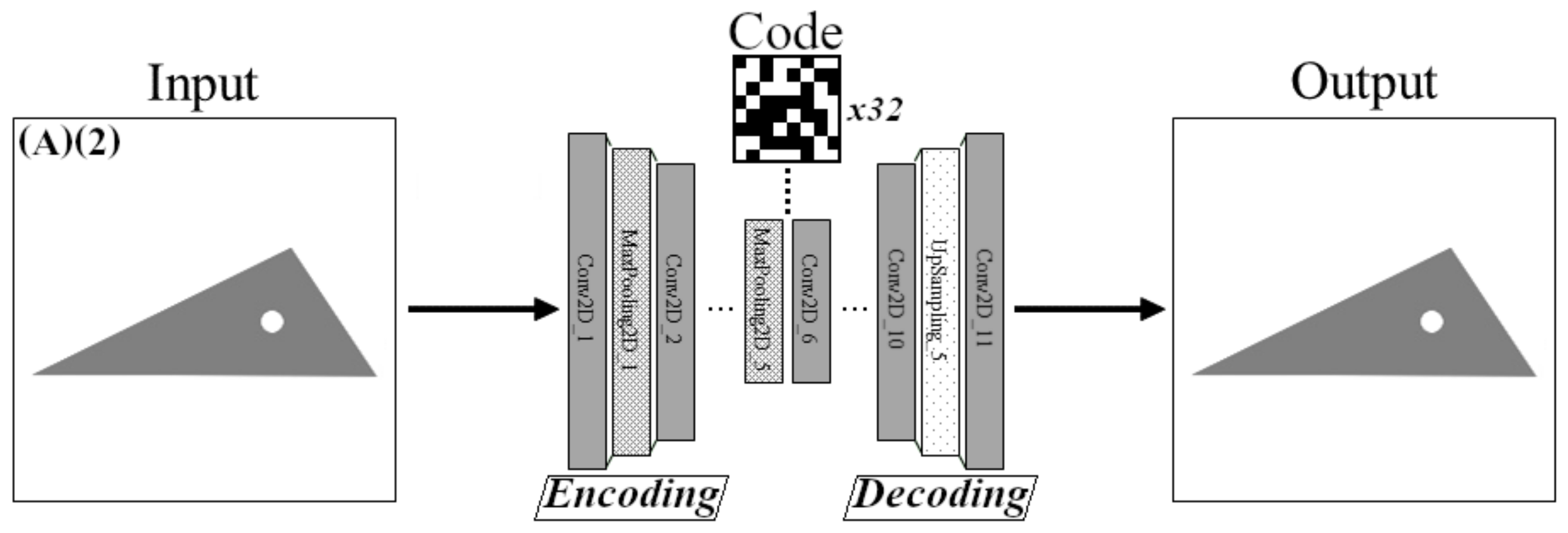
  • a training dataset made of 800 regular spotted triangles (A)(2) and a test dataset mixing 2000 defective samples (200 of each other class in the Table 1, including (A)(1))

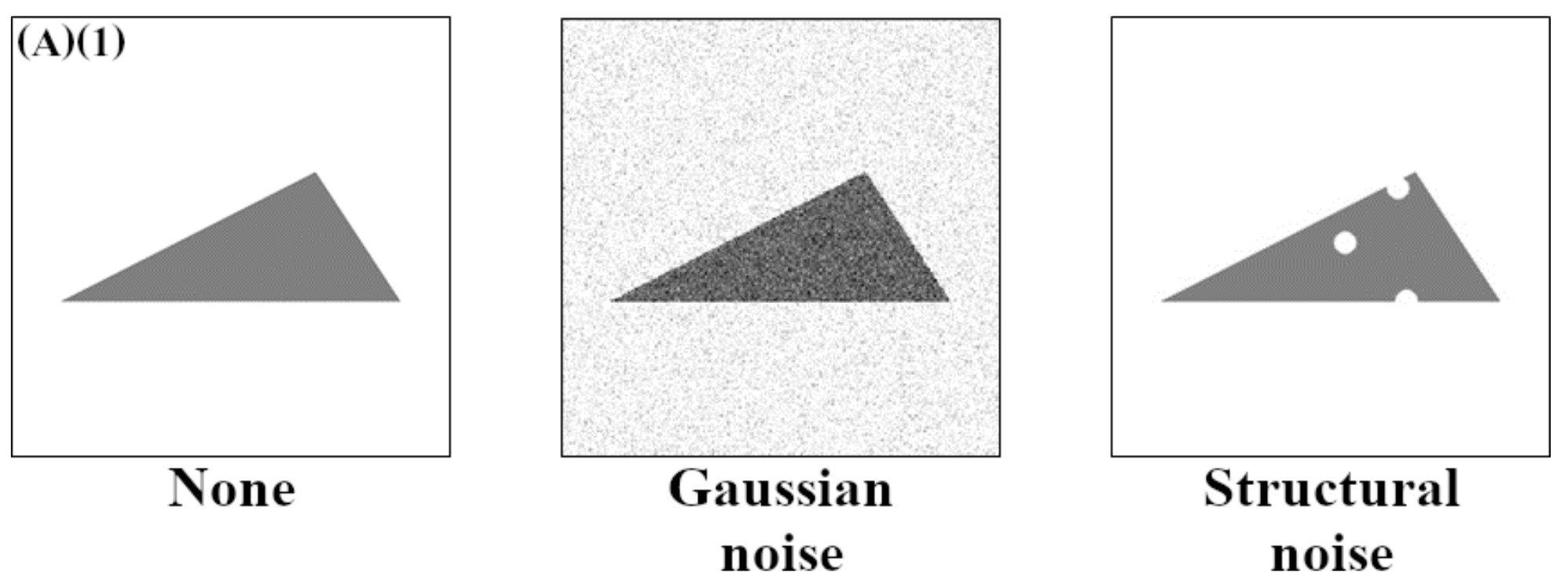
4.1.2. Noise Injection

In order to improve their encoding/decoding ability, autoencoders can be trained on data injected with some noise. These data alterations increase the versatility of NNs, their ability to handle new data that are not exactly like what they were trained on. The purpose of our study was to compare the error rates of CAEs trained on five distinct configurations: no noise, Gaussian noise, small structural noise, medium structural noise and large structural noise. Throughout our experiments, the structural noise was made of circles. In the cases of noisy trainings, the noise was added to the unaltered data before that they enter the NN. Some noisy samples are shown in Figure 9.

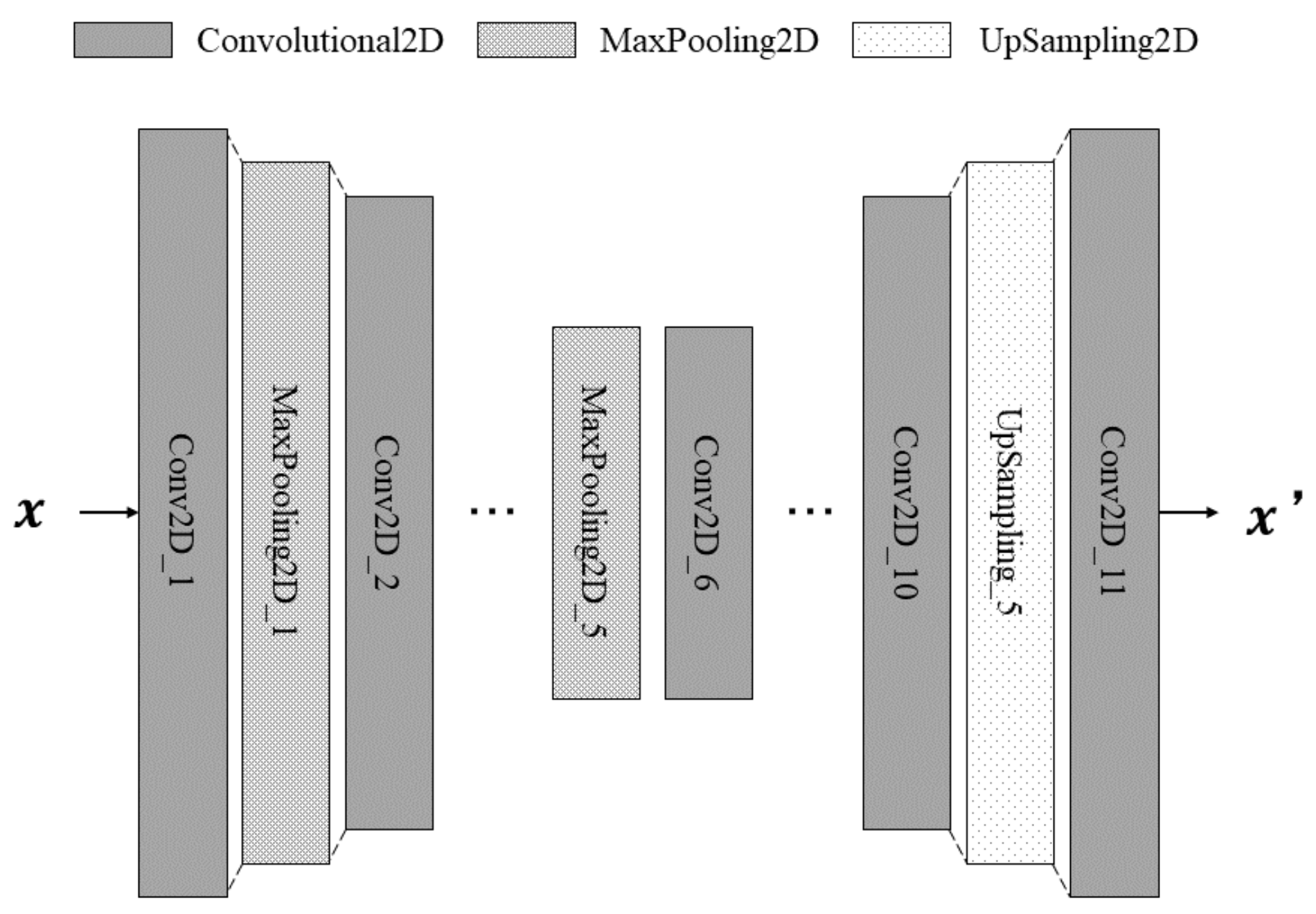
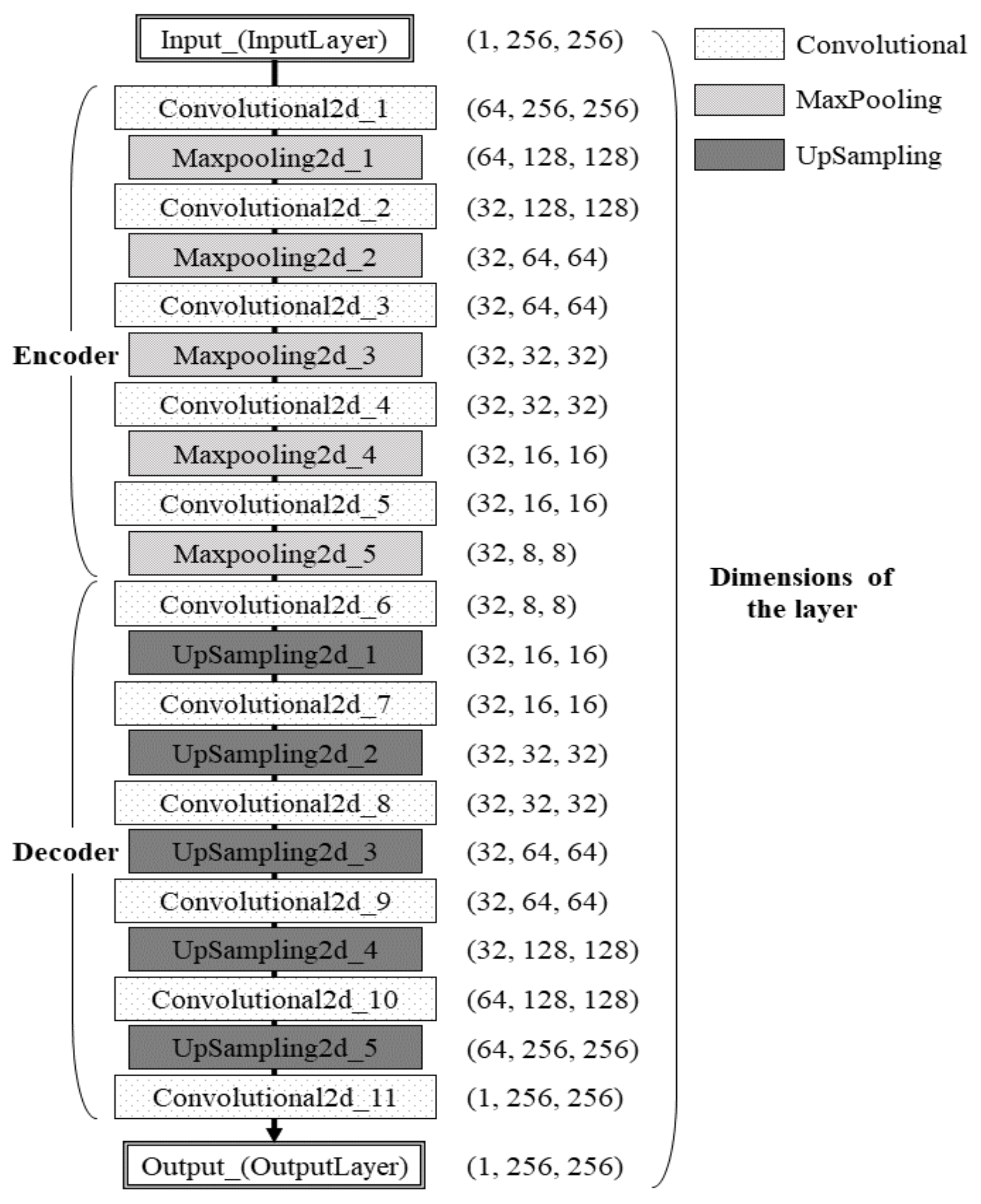
4.1.3. Network Structure

Essentially based on a common architecture among CAEs, the final structure of our neural network has been refined by “trial and error”. The Figure 10 pictures this architecture. If the training/testing data were more intricate, the network architecture would have to be adapted to process them.
The encoding phase compresses inputs from 65,536 values to 2048. Then, the decoding phase decompresses these encoded data to outputs made of 65,536 values. The sizes of the data, as well as their dimensions, change according to the filters and the operation they perform at every layer of the network. A filter can either reduce (max pooling layer) or stretch (upsampling layer) the size of data, while both the size and the dimensions are reshaped through convolutional layers. The dimension and the size of the data are indicated on the right of the layers in Figure 10. For example, data at the input and output layers are both made of 65,536 values (1 × 256 × 256), while they are made of 2048 values (32 × 8 × 8) at the end of the encoding phase.

4.2. Experimental Results

The results obtained over the course of the experiments will be explained in this section. We will attempt to verify the usefulness of our novel method for CAE-based defect detections. Overall, ten CAEs were trained, as five different training phases were conducted on each training dataset: with no noise, injected with Gaussian noise, injected with structural noise (small, medium and large sizes separately). Once again, a “trial and error” approach was used to determine the values of the hyperparameters, such as setting the batch size to 16 and the number of epochs to 300. The training phases ran until the end of the 300 predefined epochs or until the loss value fell below 0.005.

4.2.1. Models Trained without Noise

Two models resulted from the trainings with unaltered pictures.
Firstly, a model was trained on pictures without spots. The Figure 11 gives an overview of an ideal input, its structure, and a perfect output.
The differences between pieces with no defects and defective pieces were discriminated as in Figure 12.
The error rates of differences were calculated to evaluate the exactitude of the detections. Because differences are closely related to defects: the smaller the error rate, the more accurate the defect detection (and conversely). The formula used to compute the error rates is shown in Equation (1):
Error rate [ % ] = | 1 total area of differences detected [ px ] total area of differences expected [ px ] | 100
The Figure 13 shows the differences between the output and the input, after the restoration process. The bluer a pixel is within “Difference”, the blacker this pixel is within “Output” compared to “Input”, conversely, the redder a pixel is within “Difference”, the whiter this pixel is within “Output” compared to “Input”. Therefore, the whiter a pixel is within “Difference”, the more alike the pixels are within “Output” and “Input”. No particular discrepancies were observed when the inputs were similar to what the CAE is familiar with (spotless pieces), while the dissimilarities of spotted pieces were clearly highlighted. The blue disc corresponds to the spot of the spotted input that was not restored, as the NN was not trained on data including this feature. Nonetheless, a few subtle irregularities occurred in both reconstructions because the autoencoder cannot compress/decompress data without a loss of information.
Secondly, another model was trained on pictures with spots. The Figure 14 provides an overview of an ideal input, its structure, and a perfect output.
The Figure 15 also shows the differences between the output and the input, after the restoration process. The color pattern is the same as the previous input/output comparisons.No particular discrepancies were observed when the inputs were similar to what the CAE is familiar with (spotted pieces), while the dissimilarities of spotless pieces were clearly highlighted. The red disc corresponds to the “missing” spot of the spotless input that was created, as the NN was not trained on data excluding this feature. Once again, some subtle differences were noticed for the same reasons mentioned in the previous case.
Since the main purpose of this study was to detect flaws (such as scratches, spots, wrong colors or sizes), the errors caused by the restorations of the edges were dismissed from the “defective area” candidates.

4.2.2. Models Trained with Noise

In addition to the two CAE models prepared without noise, four new models were needed to investigate the possible benefits of noisy trainings.
Therefore, these NNs were trained on four distinct datasets:
  • spotless triangles (A)(1) noised by a Gaussian distribution
  • spotted triangles (A)(2) noised by a Gaussian distribution
  • spotless triangles (A)(1) noised by a known structure (medium)
  • spotted triangles (A)(2) noised by a known structure (medium)
The Gaussian noise had a mean of 0 and a standard deviation of 0.1 (the resulting values of the pixels were clamped to fit between 0 and 1). The “medium” structural noise consisted of 20 white ((r, g, b) = (255, 255, 255)) discs of radii r = 6 px, placed randomly within the injected data.
The Figure 16 and Figure 17 illustrate the noisy trainings of CAEs, on the spotless and spotted dataset, respectively. The fact that noise is injected to the data before they reach the network is clearly emphasized (Gaussian noise is added, in these instances).

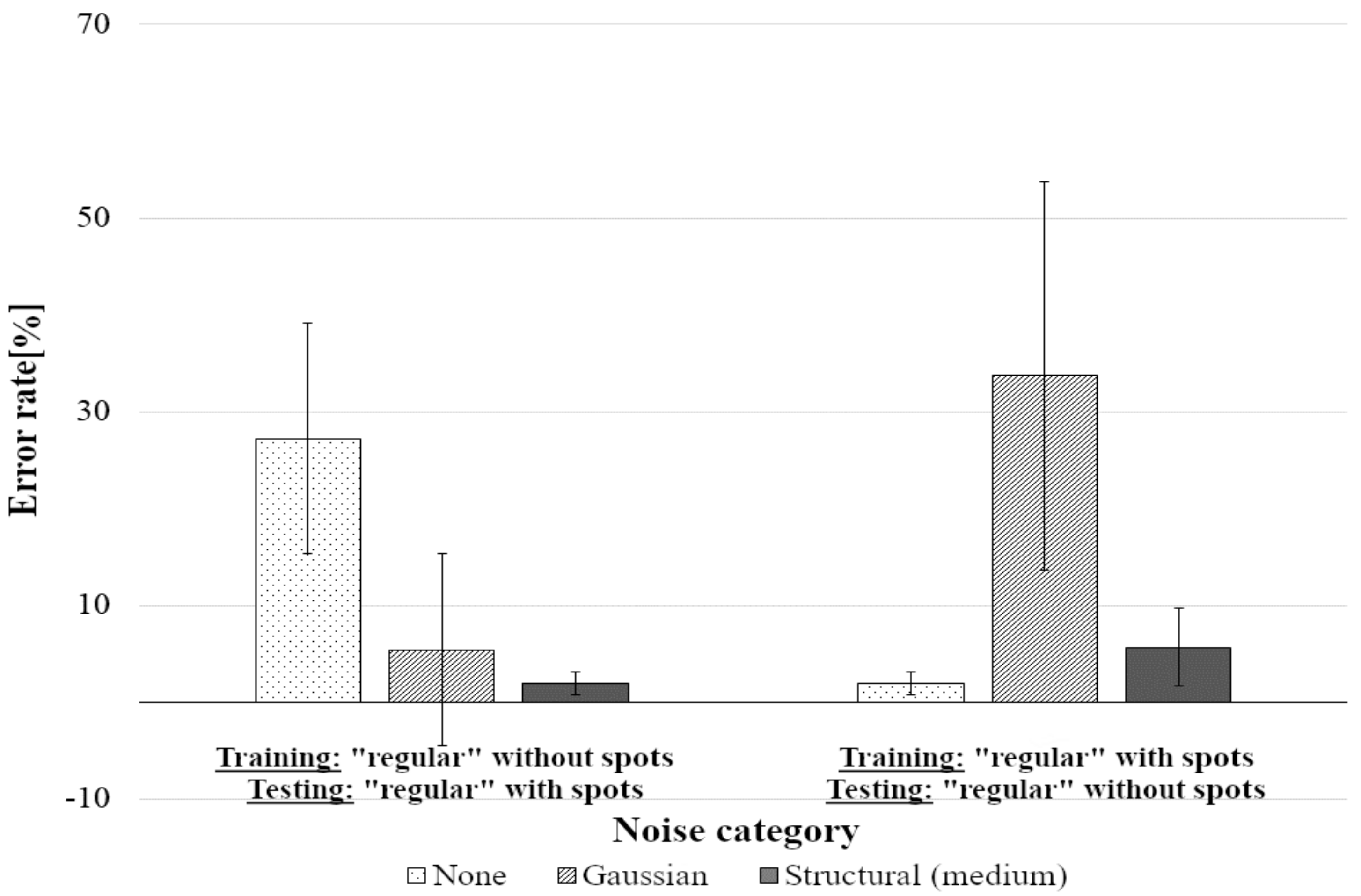
Tests on “Regular” Pictures

In the first place, the six models were tested on a sample of 200 “regular” images of the remaining dataset, i.e., the other “regular” set of images on which they were not trained. Table 2 and its corresponding Figure 18 show the outcome of these tests.
The detection accuracy clearly improved for the models trained on spotless data: while the error rate without noise was equal to 27.2%, it dropped to 5.4% with the addition of Gaussian noise and even decreased to 1.9% when structural noise was used.
The results were mixed for the models trained on spotted data: originally, without noise, the error rate was equal to 1.9% but drastically rose to 33.7% when Gaussian noise was injected, while the structural noise slightly increased the error rate to 5.7%.
Even though the results involving noise are mixed for the models trained on spotted data, the sharp gain in precision for the models trained on spotless data motivated us to further explore the path of the structural noise. At the same time, we attempted to address the small increment of the error rate for the models trained on data with spots.

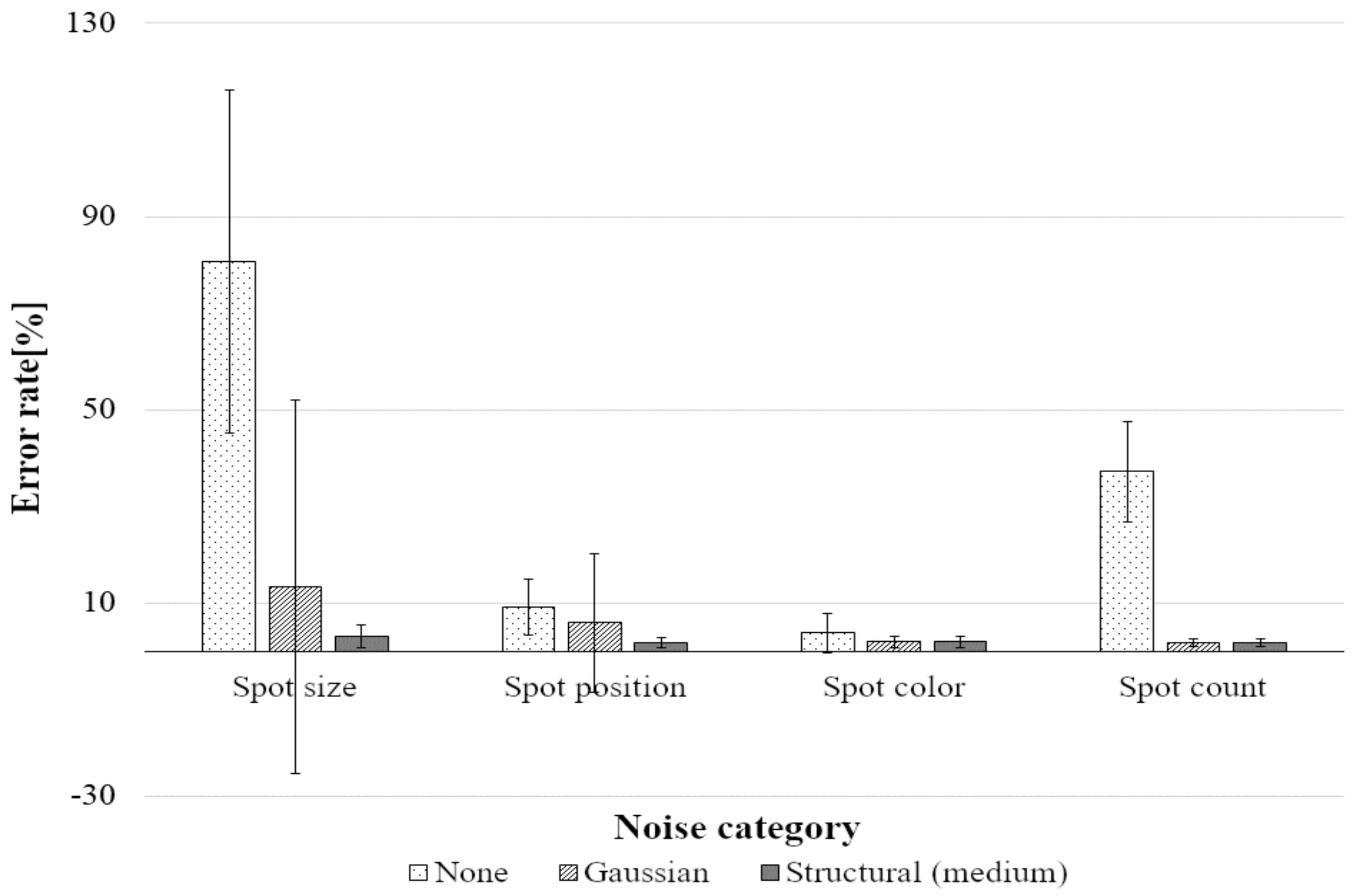
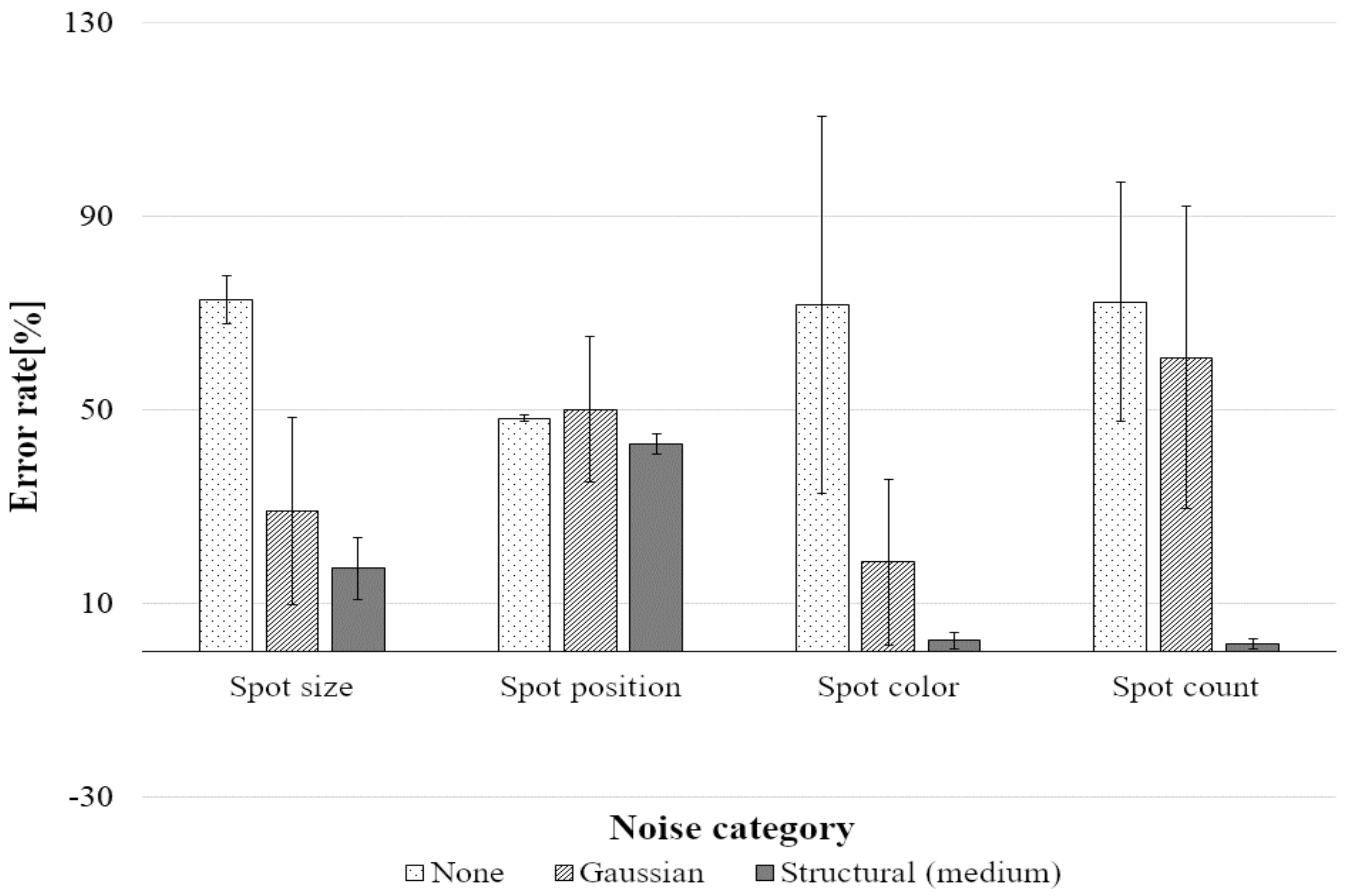
Tests on the Full Set of Data

Then, tests were conducted on a larger collection of data containing a mix of 2000 “defective” pieces, representing all of the 10 “defective” classes.
The Table 3, and its corresponding Figure 19, summarize the outcomes of the tests carried out on the models trained on the spotless dataset:
In the case of noisy training on spotless data, the restoration abilities of the CAEs definitely improved by a great margin. Using structural noise, the error rate even dropped below 5%, all tested classes combined.
The Table 4, and its corresponding Figure 20, summarize the outcomes of the tests carried out on the models trained on the spotted dataset:
According to these observations, globally, the CAEs were enhanced. The performances are rather mixed in the cases where the positions of the spots are defective, but using structural noise during training impacts positively the restoration process, in any instance.
Overall, even though the Gaussian noise increased the precision of the NNs in most cases, it clearly appeared that the noise with a known structure gave better results. The latter has particularly helped reduce the error rate when the color of the spots or their count were faulty, but was not as effective in preventing mistakes when the size of the spots or their position were problematic. It should be noted that over 50% of the defects can be detected, even in the worst situations (such as when the position of the spot is defective). The error rates may not be null, but their values are overall low enough to expose the location of the flaws.
In the case of the trainings on spotted dataset, when the position or the size of the spots are flawed, the detections may be rather unreliable due to the presence of “regular” spots inherent to the data used for these trainings. Indeed, “defective” spots (which have to be detected/removed) may partially (or totally) overlap with “regular” spots (which has to be reconstructed). In this way, as the representation in the latent space of a defective piece will be similar to that of a regular spotted piece after compression, a misinterpretation can occur during the decompression process. This confusion may lead to an increase in the error rate.

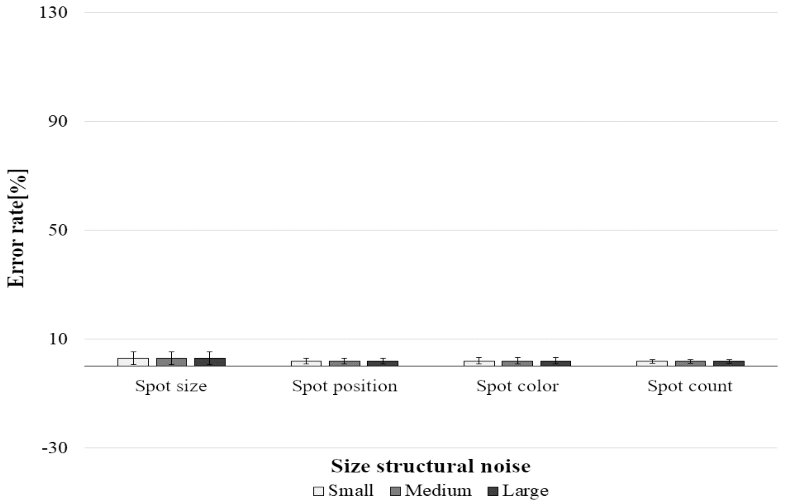
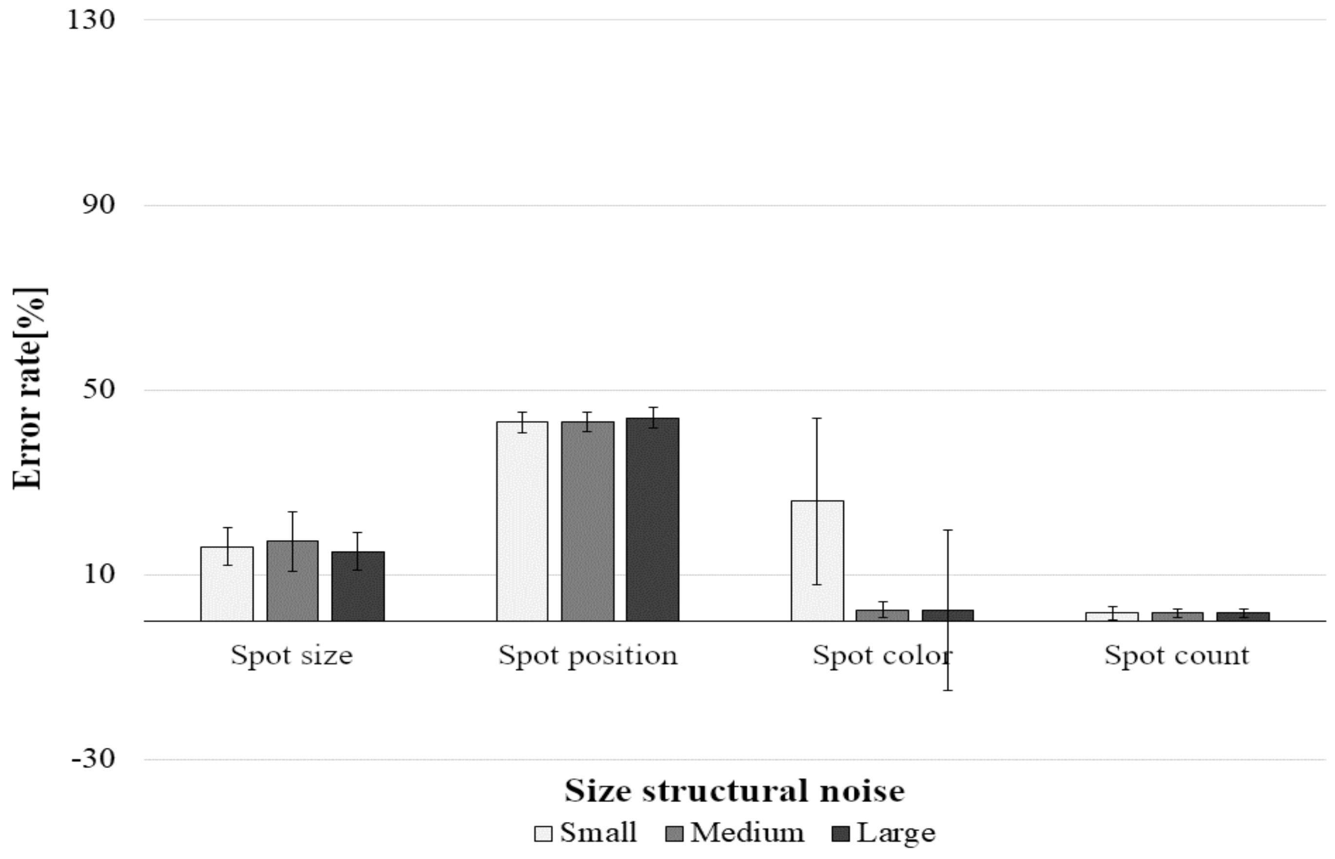
Tests on Different Sizes of Structural Noise

Finally, the effects of the patterns’ size of the structural noise on the detection accuracy were investigated.
Four additional noisy trainings were performed:
  • spotless triangles (A)(1) noised by a known structure (small)
  • spotted triangles (A)(2) noised by a known structure (small)
  • spotless triangles (A)(1) noised by a known structure (large)
  • spotted triangles (A)(2) noised by a known structure (large)
The “small” structural noise consisted of 20 white ((r, g, b) = (255, 255, 255)) discs of radii r = 3 px, whereas the “large” structural noise consisted of 20 white ((r, g, b) = (255, 255, 255)) discs of radii r = 9 px, both set of discs were placed randomly within the injected data. In total, six configurations were compared (as two models had already been trained on “medium” structural noise). The Figure 21 shows a few images injected with structural noise (for reading purpose, the “regular” spots of (A)(2) have been colored in red to distinguish them from the noise):
The results of the comparisons of the error rates are displayed in Figure 22, for the training on spotless images, and in Figure 23, for the training on spotted images. The experimentations were conducted on the respective test dataset of each training set.
On the one hand, once more, the models trained on spotless data show great detection accuracies can be observed, whatever the size of the structural noise. The error rates did not exceed 5%, regardless of the defective class to which the processed sample belonged to.
On the other hand, in a similar way, the models trained on spotted data gave mixed results. The error rates were substantial for defective spot sizes and even more problematic for defective spot positions, while low error rates were increased from the tests on samples with flawed spot colors and counts. In addition, concerning standard deviations appeared for the error rates when images with flawed spot colors where processed by the models trained on small and large noise structures.
The error rates were still higher for the tests on irregular spot sizes and positions, as the problem mentioned in the previous battery of tests remained.

5. Conclusions

This study introduced a CAE-based defect detector improved thanks to structural noise added during its training phase. Furthermore, the models generated through our method were trained on flawless data and were able to detect anomalies on defective data, even when their positions and orientations differed from that of the training set. Throughout our experiments, it was proven that a training set injected with structural noise gave better results than that with Gaussian noise or with no noise at all. In general, the image restoration improved and the detection of defects increased, but some issues persist when “regular” pictures contain spots that would later overlap with anomalous spots within “defective” pictures. This study would benefit from testing on an even greater number of patterns of structural noise, which could potentially further improve the efficiency of the models.

Author Contributions

Conceptualization, O.F. and R.M.; Methodology, R.M. and O.F.; Software, R.M.; Validation, O.F.; Formal analysis, R.M.; Investigation, R.M.; Resources, R.M. and O.F.; Data curation, R.M. and V.G.; Writing—original draft preparation, V.G. and R.M.; Writing—review and editing, V.G. and O.F.; Visualization, R.M. and V.G.; Supervision, O.F., H.O. and N.Y.; Project administration, O.F.; Funding acquisition, O.F. All authors have read and agreed to the published version of the manuscript.

Funding

This research was supported by Adaptable and Seamless Technology transfer Program through Target-driven R&D (A-STEP), Japan Science and Technology Agency (JST).

Institutional Review Board Statement

Not applicable.

Informed Consent Statement

Not applicable.

Data Availability Statement

Not applicable.

Conflicts of Interest

The funders had no role in the design of the study; in the collection, analyses, or interpretation of data; in the writing of the manuscript, or in the decision to publish the results.

References

  1. See, J.E.; Drury, C.G.; Speed, A.; Williams, A.; Khalandi, N. The Role of Visual Inspection in the 21st Century. Proc. Hum. Factors Ergon. Soc. Annu. Meet. 2017, 61, 262–266. [Google Scholar] [CrossRef]
  2. Szeliski, R. Computer Vision: Algorithms and Applications, 1st ed.; Springer: London, UK, 2011; pp. 578–631. [Google Scholar]
  3. Goudail, F.; Lange, E.; Iwamoto, T.; Kyuma, K.; Otsu, N. Fast face recognition method using high order autocorrelations. In Proceedings of the International Conference on Neural Networks (1993), Nagoya, Japan, 25–29 October 1993; Volume 2, pp. 1297–1300. [Google Scholar]
  4. Chauhan, A.P.S.; Bhardwaj, S.C. Detection of Bare PCB Defects by Image Subtraction Method using Machine Vision. In Proceedings of the World Congress on Engineering (2011), London, UK, 6–8 July 2011; Volume 2. [Google Scholar]
  5. Elgendy, M. Deep Learning for Vision Systems, 1st ed.; Manning Publications Co.: Shelter Island, NY, USA, 2020; pp. 27–33. [Google Scholar]
  6. Kattan, M.W. Encyclopedia of Medical Decision Making, 1st ed.; SAGE Publications: Thousand Oaks, CA, USA, 2009; pp. 323–328. [Google Scholar]
  7. Cristianini, N.; Shawe-Taylor, J. An Introduction to Support Vector Machines and Other Kernel-based Learning Methods, 1st ed.; Cambridge University Press: Cambridge, UK, 2000; pp. 93–124. [Google Scholar]
  8. Chen, Z.; Yeo, C.K.; Lee, B.S.; Lau, C.T. Autoencoder-based network anomaly detection. In Proceedings of the Wireless Telecommunications Symposium (WTS), Phoenix, AZ, USA, 18–20 April 2018; pp. 1–5. [Google Scholar]
  9. Vincent, P.; Larochelle, H.; Bengio, Y.; Manzagol, P. Extracting and Composing Robust Features with Denoising Autoencoders. In Proceedings of the 25th International Conference on Machine Learning (ICML ’08), Helsinki, Finland, 5–9 July 2008; pp. 1096–1103. [Google Scholar]
  10. Vincent, P.; Larochelle, H.; Lajoie, I.; Bengio, Y.; Manzagol, P. Stacked Denoising Autoencoders: Learning Useful Representations in a Deep Network with a Local Denoising Criterion. J. Mach. Learn. Res. 2010, 11, 3371–3408. [Google Scholar]
  11. Mao, X.-J.; Shen, C.; Yang, Y.-B. Image Restoration Using Very Deep Convolutional Encoder-Decoder Networks with Symmetric Skip Connections. In Proceedings of the 30th International Conference on Neural Information Processing Systems (NIPS’16), Barcelona, Spain, 5–10 December 2016; pp. 2810–2818. [Google Scholar]
  12. Inayoshi, H.; Kurita, T. Improved Generalization by Adding both Auto-Association and Hidden-Layer-Noise to Neural-Network-Based-Classifiers. In Proceedings of the IEEE Workshop on Machine Learning for Signal Processing, Mystic, CT, USA, 28–30 September 2005; pp. 141–146. [Google Scholar]
  13. Poole, B.; Sohl-Dickstein, J.; Ganguli, S. Analyzing noise in autoencoders and deep networks. arXiv 2014, arXiv:1406.1831. [Google Scholar]
  14. Meng, X.; Liu, C.; Zhang, Z.; Wang, D. Noisy training for deep neural networks. In Proceedings of the IEEE China Summit and International Conference on Signal and Information Processing (ChinaSIP), Xi’an, China, 9–13 July 2014; pp. 16–20. [Google Scholar]
  15. An, G. The effects of adding noise during backpropagation training on a generalization performance. Neural Comput. 1996, 8, 643–674. [Google Scholar] [CrossRef]
  16. Grandvalet, Y.; Canu, S.; Boucheron, S. Noise injection: Theoretical prospects. Neural Comput. 1997, 9, 1093–1108. [Google Scholar] [CrossRef]
  17. DeVries, T.; Taylor, G.W. Improved Regularization of Convolutional Neural Networks with Cutout. arXiv 2017, arXiv:1708.04552. [Google Scholar]
  18. Zhong, Z.; Zheng, L.; Kang, G.; Li, S.; Yang, Y. Random Erasing Data Augmentation. In Proceedings of the AAAI Conference on Artificial Intelligence, New York, NY, USA, 7–12 February 2020; pp. 13001–13008. [Google Scholar]
Figure 1. Structure of a classical autoencoder.
Applsci 11 12062 g001
Figure 2. Succession of layers within our CAE.
Applsci 11 12062 g002
Figure 3. Hypothetical restorations performed by an advanced CAE.
Applsci 11 12062 g003
Figure 4. Detection of differences.
Applsci 11 12062 g004
Figure 5. Restoration performed by a CAE trained on data without noise.
Applsci 11 12062 g005
Figure 6. Restoration performed by a CAE trained on data with noise.
Applsci 11 12062 g006
Figure 7. Some samples from each dataset.
Applsci 11 12062 g007
Figure 8. Examples of rotations, on both regular data: spotless (A)(1) and spotted (A)(2).
Applsci 11 12062 g008
Figure 9. Different noises used for training (here, on a regular spotless piece (A)(1)).
Applsci 11 12062 g009
Figure 10. Architecture of our autoencoders.
Applsci 11 12062 g010
Figure 11. Classic CAE training on spotless pieces.
Applsci 11 12062 g011
Figure 12. Differences expected versus differences detected.
Applsci 11 12062 g012
Figure 13. Reconstruction of samples after training.
Applsci 11 12062 g013
Figure 14. Classic CAE training on spotted pieces.
Applsci 11 12062 g014
Figure 15. Reconstruction of samples after training.
Applsci 11 12062 g015
Figure 16. Noisy CAE training on spotless pieces.
Applsci 11 12062 g016
Figure 17. Noisy CAE training on spotted pieces.
Applsci 11 12062 g017
Figure 18. Comparison of detection error rates [%] obtained by the six models during the tests, according to the type of noisy training.
Applsci 11 12062 g018
Figure 19. Comparison of detection error rates [%] for the models trained on spotless parts, according to the type of noisy training.
Applsci 11 12062 g019
Figure 20. Comparison of detection error rates [%] for the models trained on spotted parts, according to the type of noisy training.
Applsci 11 12062 g020
Figure 21. Examples of images injected with different sizes of structural noise.
Applsci 11 12062 g021
Figure 22. Comparison of detection error rates [%] for the models trained on spotless parts, according to the size of the structural noise.
Applsci 11 12062 g022
Figure 23. Comparison of detection error rates [%] for the models trained on spotted parts, according to the size of the structural noise.
Applsci 11 12062 g023
Table 1. Compositions of the training and test datasets.
CategoryClassParameter
(A) Presence of a spot(1) Without a spot-
(2) With a spotSpot radius r = 25 px
(B) Defective spot size(1) SmallSpot radius r = 12.5 px
(2) Largespot radius r = 37.5 px
(C) Defective spot position(1) UpSpot position 25 px to the top
(2) DownSpot position 25 px to the bottom
(3) LeftSpot position 25 px to the left
(4) RightSpot position 25 px to the right
(D) Defective spot color(1) BlackSpot color (r, g, b) = (0, 0, 0)
(E) Defective spot count(1) Two2 spots
(2) Three3 spots
Table 2. Detection error rates [%] obtained by the six models during the tests, according to the type of noisy training.
Additive Noise
NoneGaussianStructural
Training
dataset
Without spots27.25.41.9
With spots1.933.75.7
Table 3. Detection error rates [%] for the models trained on spotless parts, according to the type of noisy training.
Defect
Spot SizeSpot PositionSpot ColorSpot Count
SmallLargeUpDownLeftRightBlackTwoThree
Category
of
noise
None50.2111.09.19.89.18.33.927.946.1
Gaussian2.024.55.26.18.34.12.01.91.8
Structural1.44.62.01.91.71.82.01.91.7
Table 4. Detection error rates [%] for the models trained on spotted parts, according to the type of noisy training.
Defect
Spot SizeSpot PositionSpot ColorSpot Count
SmallLargeUpDownLeftRightBlackTwoThree
Category
of
noise
None77.568.148.348.348.248.271.847.396.6
Gaussian25.233.044.070.936.948.318.687.243.6
Structural15.918.543.143.043.742.52.31.71.7
Publisher’s Note: MDPI stays neutral with regard to jurisdictional claims in published maps and institutional affiliations.

