Article

Image Reconstruction Using Autofocus in Single-Lens System

School of Physics, Harbin Institute of Technology, Harbin 150001, China
*
Author to whom correspondence should be addressed.
Appl. Sci. 2022, 12(3), 1378; https://doi.org/10.3390/app12031378
Submission received: 18 December 2021 / Revised: 24 January 2022 / Accepted: 25 January 2022 / Published: 27 January 2022
(This article belongs to the Special Issue Advances in Digital Image Processing)

Abstract

:
To reconstruct the wavefront in a single-lens coherent diffraction imaging (CDI) system, we propose a closed-loop cascaded iterative engine (CIE) algorithm based on the known information of the imaging planes. The precision of diffraction distance is an important prerequisite for a perfect reconstruction of samples. For coherent diffraction imaging with a lens, autofocus is investigated to accurately determine the object distance and image distance. For the case of only the object distance being unknown, a diffuser is used to scatter the coherent beam for speckle illumination to improve the performance of autofocus. The optimal object distance is obtained stably and robustly by combing speckle imaging with clarity evaluation functions. SSIM and MSE, using the average pixel value of the reconstructed data set as a reference, are applied on two-unknown-distance autofocus. Simulation and experiment results are presented to prove the feasibility of the CIE and proposed auto-focusing method.

1. Introduction

In computational imaging, phase retrieval (PR) is a tool to reconstruct a wavefront with diffraction images [1,2,3,4,5,6]. Recently, multi-intensity iterative algorithms [7,8,9,10] have shown stronger noise robustness, however, it is easy to bring an aliasing artifact into the system. Here the diffraction intensity patterns of an object at different distances are employed to improve the convergence of phase retrieval [11,12,13,14,15,16,17,18]. The single-beam, multiple-intensity reconstruction (SBMIR) algorithm [10] belongs to serial iteration. The amplitude-phase retrieval (APR) [16] is a parallel iterative algorithm that renews the complex amplitude of the target with the average of calculated data. The above iterative algorithms have been used to reconstruct the wavefront in CDI [17,18].
For diffraction integral models, such as angular spectrum and Fresnel diffraction, distance is a sensitive parameter for the quality of a reconstructed image. Especially in computational microscopies, higher imaging quality requires a more accurate measurement of the distance between optical elements. If the diffraction distance is inaccurate, the overall sharpness of the image will decline and the phenomenon of defocusing will occur [19,20]. Thus, auto-focusing algorithms were considered to search for an optimal position in imaging systems [21,22,23,24]. Clarity evaluation functions (CEFs) are defined by derivative, statistics, histogram, and some intuitive algorithms [25,26,27,28,29]. A well-established CEF comprises the numerical refocusing (propagation) of the recorded diffraction patterns to a set of distances and evaluating the quality of the propagated field using so-called focus metrics. The distance corresponding to the maximum or minimum of the CEF curve is considered as the indicator of the focal plane [30,31,32]. Different CEFs are adapted to sample images of different pixel types [33]. In a single-lens system, the autofocus of the object distance and image distance finds the mountain peak in two-dimensional space simultaneously.
Firstly, we propose a cascaded iterative engine (CIE) based on the characteristics of single-lens CDI in this paper. The iterative process is only carried out on the diffraction plane without considering the modulation effect of the lens and the unknown object and image distances in the system. The reconstructed image is obtained after the one-time inverse diffraction and the lens modulation of the iterative result. According to the idea of serial iteration and parallel iteration, the CIE can be divided into serial CIE (SCIE) and parallel CIE (PCIE). SCIE shows good convergence characteristics and robustness. Secondly, for a case in which image distance is the only unknown parameter, the diffraction patterns are recorded from the back focal plane of the lens. We insert a diffuser into the system and combine the classic CEFs to accurately obtain the object distance. Speckle illumination improves the sensitivity and accuracy of autofocus in a single-lens CDI as compared to coherent illumination. Thirdly, in the case that both the distances are unknown, we use two error functions, mean squared error (MSE) and structural similarity (SSIM) as CEF to obtain the object distance and image distance simultaneously. This method realizes the accurate acquisition of the auto-focusing curves in three-dimensional space. Simulations and experiments have been performed to test the performance of the auto-focusing scheme.

2. Methodology

The experimental layout of distance scanning and computational imaging is given in Figure 1. The system is mainly composed of four parts: fiber-optic laser with collimating lens, diffuser, single lens, and scientific CCD. The scanning operation of object distance z 1 is achieved by changing the position of the lens.
The scattered light through D irradiates the sample and travels a distance z 0 in the free space. The beam is further modulated by the lens L 2 , and then the diffraction images are recorded by CCD at the distance z 2 . For autofocus, a set of speckle images are recorded and used to scan the distance z 1 by CEFs. Here the first recorded position is the back focal plane of the lens L 2 . For sample reconstruction, coherent illumination is applied for recording diffraction patterns. The first image I 0 is recorded at the focal plane of L 2 , and the others are recorded outside the back focal plane. The images recorded by coherent illumination will be used for image reconstruction after the auto-focusing task is completed.

2.1. Autofocus and Iterative Algorithm

Based on the single-lens CDI system in Figure 1, the insertion and removal of the diffuser realize the switch of speckle illumination and coherent illumination. In this paper, speckle illumination is used to realize autofocus and coherent illumination is used for image construction. The flowchart is given in Figure 2, which includes three parts:
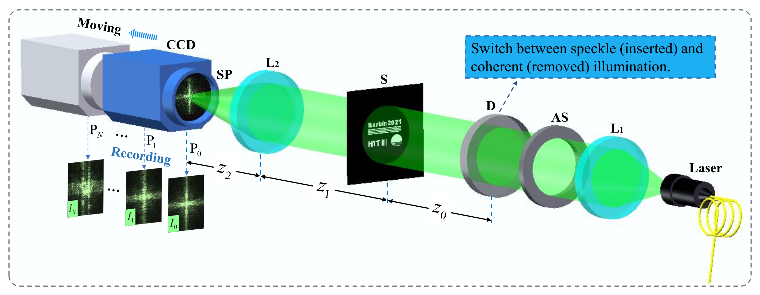
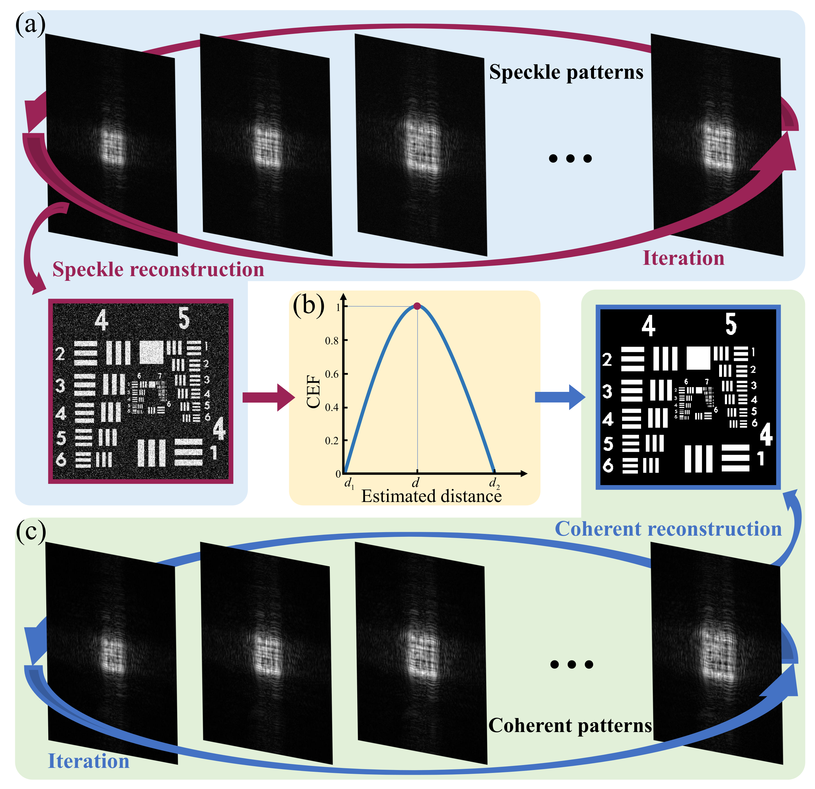
  • Reconstruction of the scattered out-of-focus dataset by using the intensity patterns under speckle illumination.
  • Clarity evaluation of reconstructed speckle images, and curve drawing between estimated distances and clarity results.
  • Reconstruction of coherent patterns by using the quasi-focus distance in step 2.

2.2. Clarity Evaluation Function

Clarity can be used as the standard of image evaluation [34]. The clarity evaluation index produces an extreme value (maximum or minimum value) only for the focused plane in an imaging system [30,33]. In this section, CEFs are utilized to evaluate the object distance z 1 . We apply different auto-focusing criterias to estimate the position of a retrieved sample as CEF. The expressions are written as follows [23,35,36],
GRA z = I z d x d y ,
LAP z = 2 I z 2 d x d y ,
SG ( z ) = [ I ( z ) ] 2 d x d y
SPEC z = ln 1 + F I ( z ) I ¯ ( z ) d x d y ,
TOG ( z ) = std ( | i ( z ) | ) / mean ( | i ( z ) | ) , i ( z ) = I ( z ) ,
Brenner ( z ) = x y I ( x + 2 , y , z ) I ( x , y , z ) 2 ,
Entropy ( z ) = i = 0 L 1 p i ln p i ,
VAR ( z ) = x y | I ( z ) I ¯ ( z ) | 2 ,
AM ( z ) = 1 M N | I ( x , y , z ) | ,
where ∇ is the gradient operator. · is the modulus operator. The functions ‘std’ and ‘mean’ are the standard deviation and mean calculation. CEF is regarded as auto-focusing metrics by searching its maximum or minimum. In this paper, instead of creating new CEFs, we combine speckle illumination with CEFs to make existing auto-focusing algorithms more stable and robust. Since the speckle illumination mode makes a re-distribution of gradient data on recording planes.

2.3. Image Reconstruction
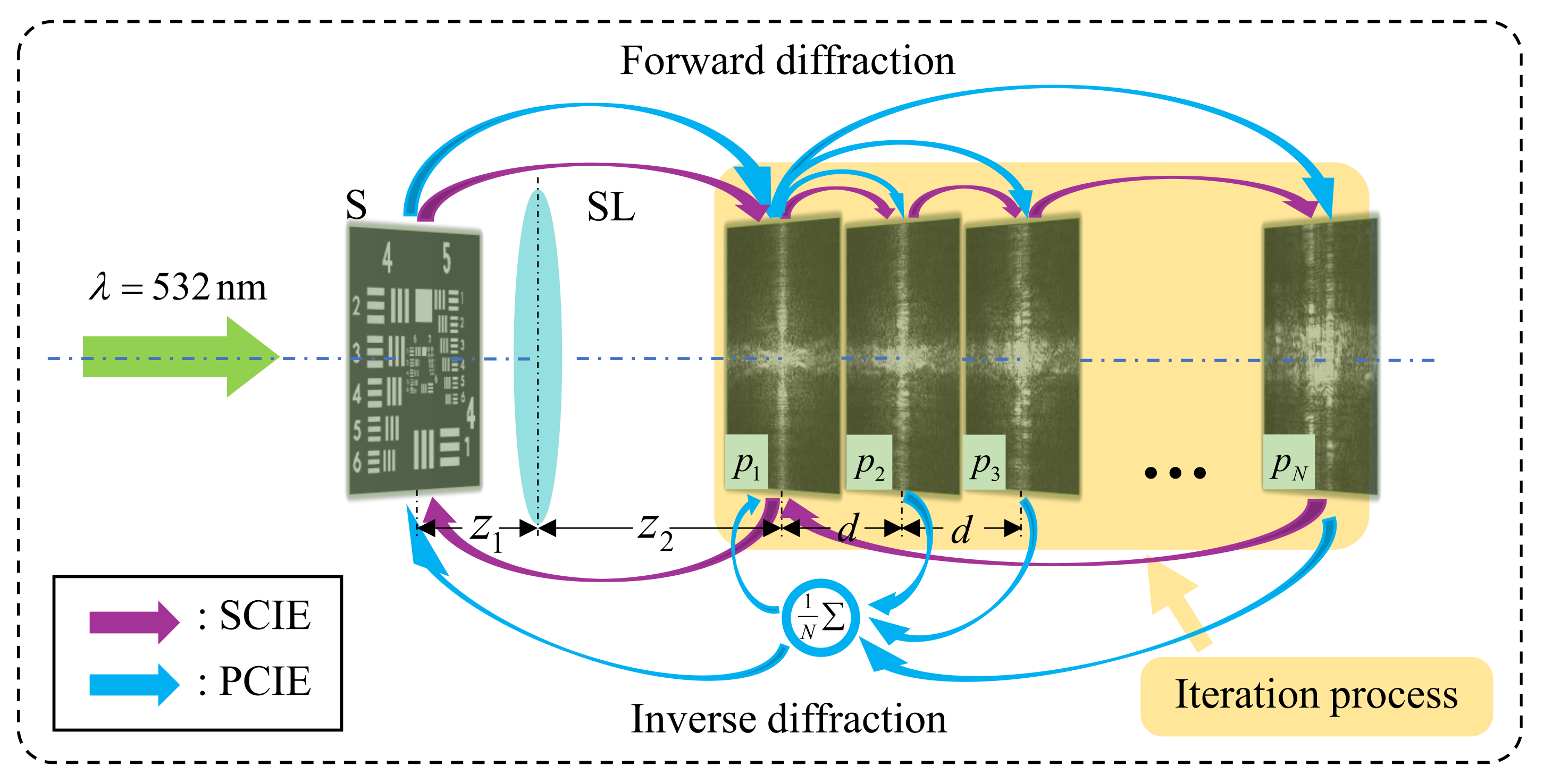
In lensless CDI, iterative calculations start from the sample plane after assuming the amplitude and phase of the sample. In single-lens CDI, for our CIE, only the known information is used for iteration. The sample, object distance, and image distance are not considered during iteration, and the modulation effect of the lens is temporarily avoided. The result of the iteration is the diffraction image on the first recoding plane, and the reconstructed sample is obtained after inverse diffraction and lens modulation. The process of PCIE is is given as follows: (1) We use the square root of the intensity pattern on the first recording plane while keeping the phase information unchanged; (2) Forward propagation in turn until all recording planes are traversed; (3) Inverse diffraction propagation to the first recording plane; (4) The above iterative process is repeated to obtain the reconstructed first recording plane diffraction image; (5) Inverse diffraction propagation to the object plane to obtain the reconstructed sample image, as shown by the purple arrows in Figure 3. In SCIE, the diffraction patterns of each recording plane are processed separately, and the estimated average values are used as the output result of each iteration. Finally, it is inverse-diffracted to the object plane as shown by the blue arrows in Figure 3.
The procedure of the CIE is represented as follows:
(1)
I n represents the pattern of scattered illumination on n-th imaging plane recorded by CCD. U n k exp ( i β n k ) represents the k-th complex-value guess when the image is on the n-th plane.
(2)
The light field functions of two adjacent imaging surfaces are propagated by the angular spectrum method as
U n k exp i β n k = A d U n 1 k exp i β n 1 k ,
where A d is forward angular spectrum propagation operator with a distance d. During the iteration, the real part U n k exp i β n k of k-th complex-value guess on the plane P n is replaced by the root of measured intenisty I n . The intervals between the adjacent detecting positions are equal in simulations and experiments.
(3)
When the iteration runs on the last diffraction plane n = N , the synthesized complex amplitude propagates backward to the first plane P 0 . And, A N d represents the backforward angular spectrum propagation operator. The complex amplitude at the plane P 0 is replaced with
U 0 k + 1 exp i β 0 k + 1 = A N d U N k exp i β N k .
Steps (2) and (3) will be implemented iteratively.
(4)
Convergence evaluation criteria in the current loop is achieved by the function
Δ min = U n n I n n ,
The above steps describe the process of closed loop iteration. Based on the data set retrieved above, the auto-focusing process is listed as follows:
(i)
A specific range for object distance is selected for covering the actual distance.
(ii)
Supposing that U exp i β is the complex amplitude at the plane P 0 after M iterations, the complex amplitude of sample is obtained by back propagation and is expressed as
U L x L , y L = A z 2 U x , y exp i β x , y ,
U S x S , y S = A z 1 t x L , y L U L x L , y L ,
where U L and U S are complex amplitudes at the plane P L and the sample plane, respectively. The function t ( x , y ) is the phase of the lens L 2 .
(iii)
By changing the distance z 1 , several recovered complex amplitudes of sample are obtained with U S n at the distance d n , which is given as
d n = d s + n 1 Δ d ,
where d s and Δ d represent starting distance and interval.
Finally, the object distance is sought by the operation on CEF as
z 1 = find d n = CEF U S n 2 .
The speckle illumination has superiority compared with coherent light for autofocus. Coherent illumination, however, can receive the reconstructed image with higher quality than the speckle case in our single-lens CDI, because speckle illumination will drown out the details and sharp edges of the sample image [37]. Thereby, coherent illumination is utilized for imaging. A set of diffraction intensity images by coherent illumination are recorded, when the diffuser is removed from the optical system. The complex amplitude of the sample can be retrieved by repeating the above iterative process with the evaluated distance z 1 calculated by step (iii).
The above steps are the serial iterative process. For the parallel process, the complex amplitudes are changed as
U n k exp i β n k = A S A n 1 exp i β n 1 k 1 ,
U 1 k + 1 exp i β 1 k + 1 = 1 N n = 1 N A N d A n exp i β n k ,
where A n ( n = 2 , 3 , , N ) is intensity images recorded from coherent illumination. The purple and blue arrows represent the iterative process of SCIE and PCIE respectively in Figure 3.

2.4. Speckle Model

The speckle model is given in the numerical simulation. Considering the phase modulation effect of the lens in the actual optical path, we simulate speckle illumination in complex form as
Pattern = A z 0 exp i 3 π 2 R a n d M × N ,
where A z 0 represents forward angular spectrum propagation operator with a distance z 0 . R a n d M × N is a random binary matrix.

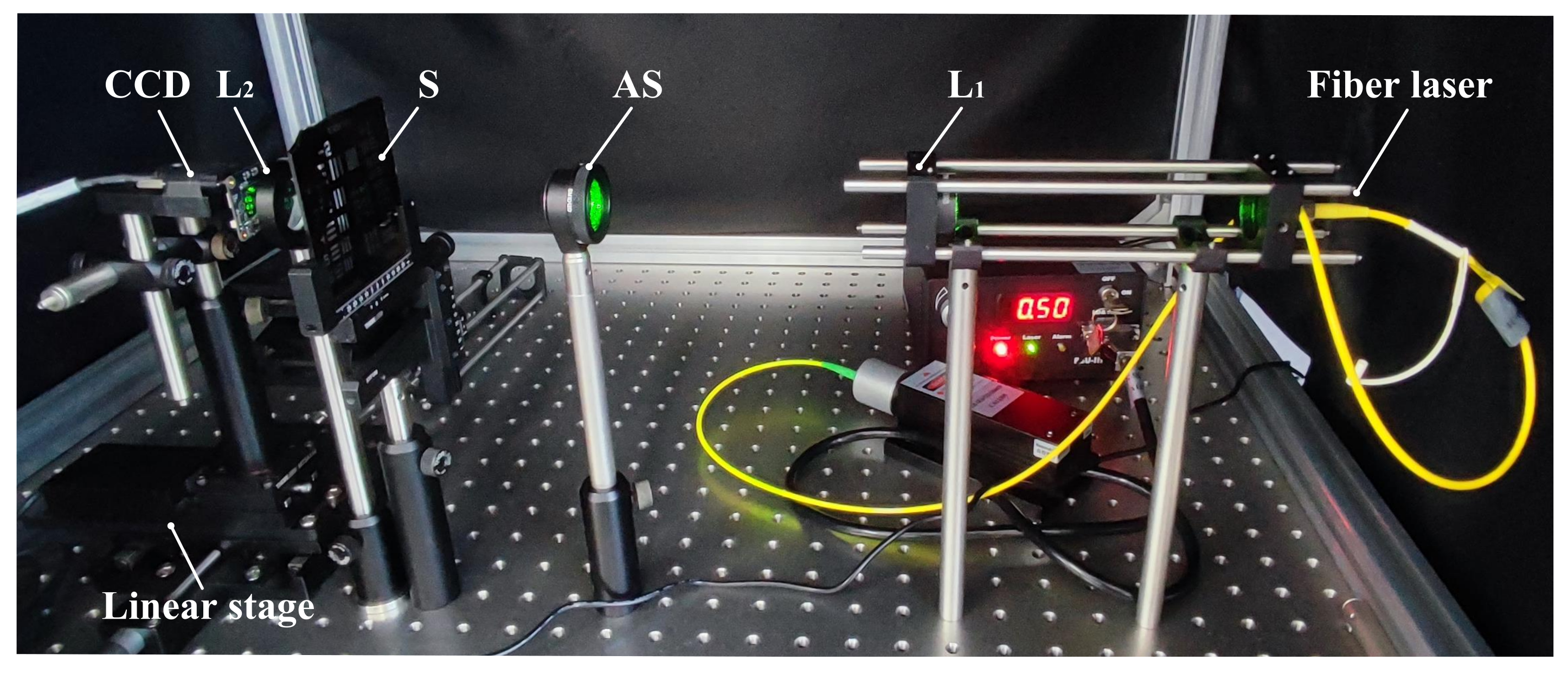
3. Simulation and Experiments

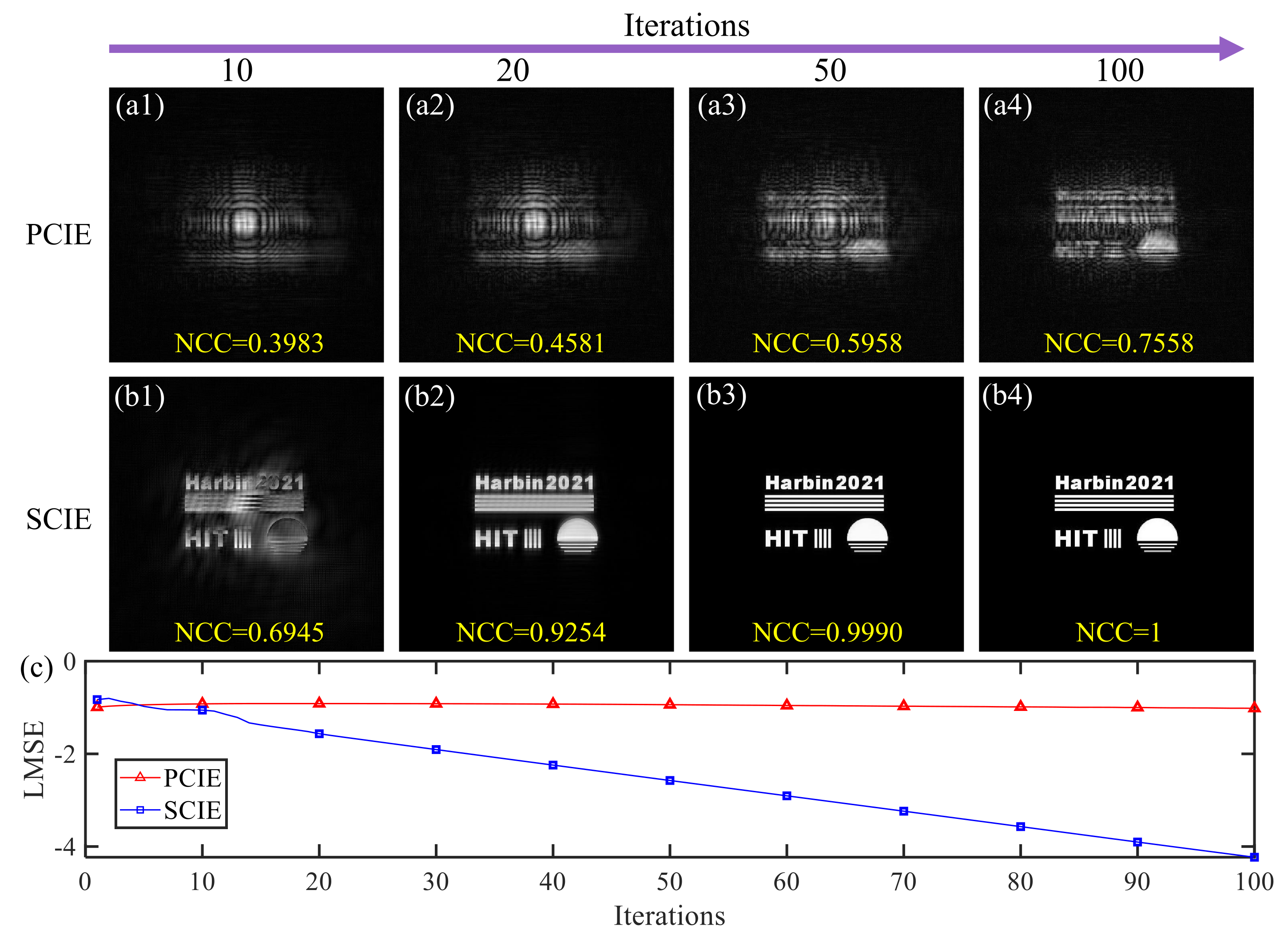
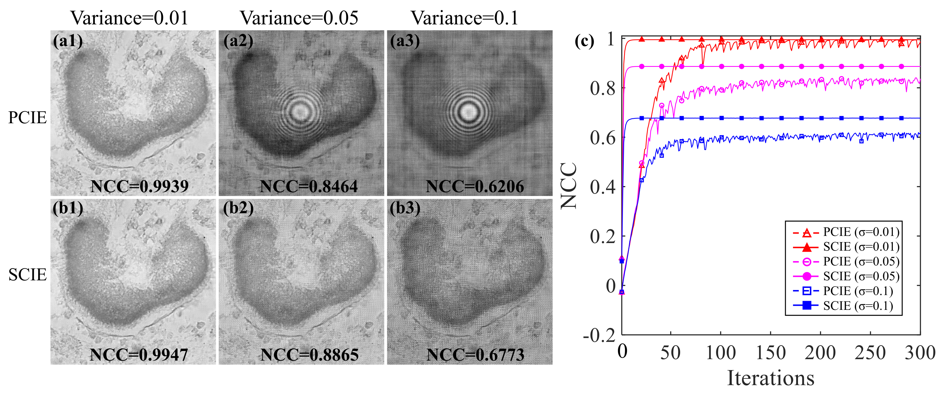
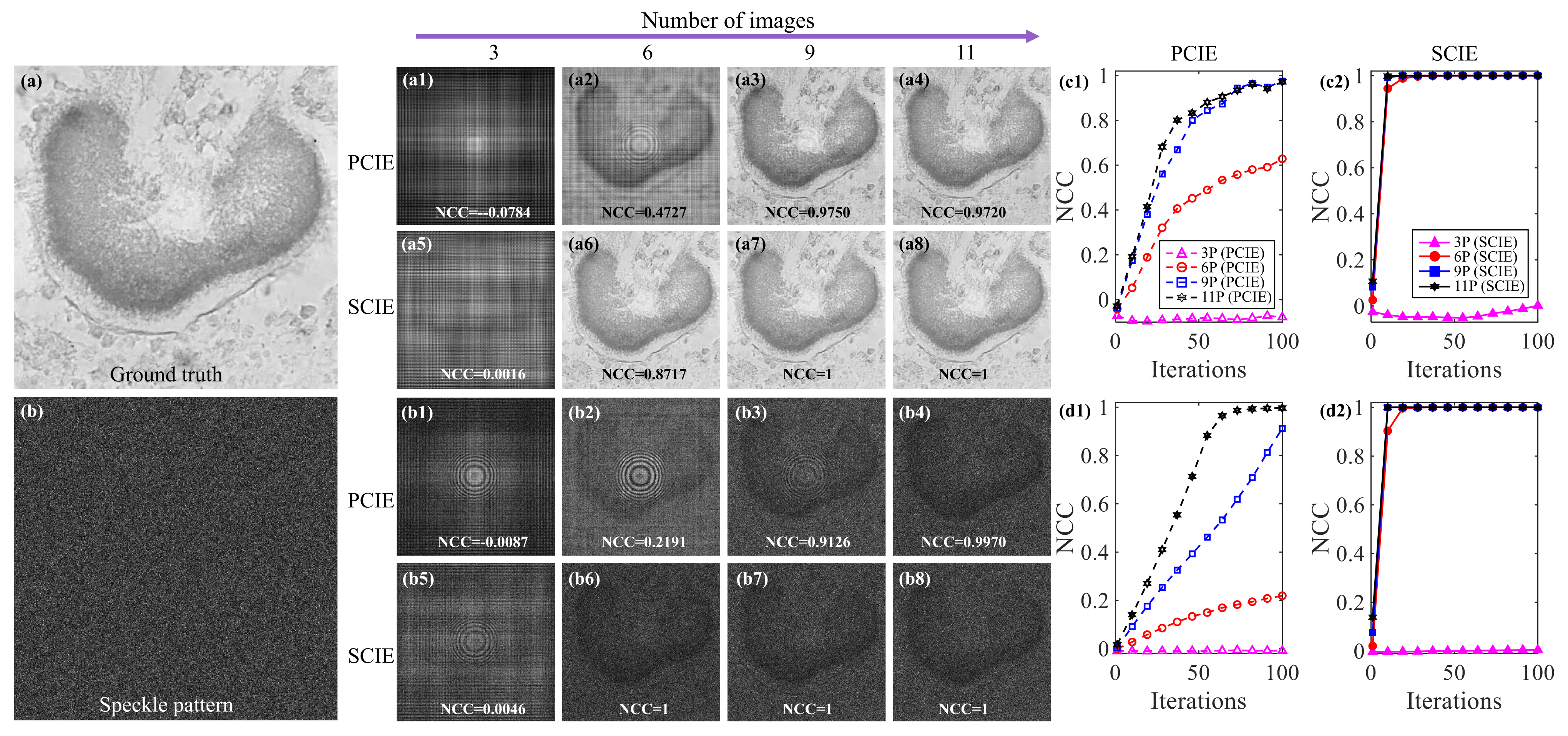
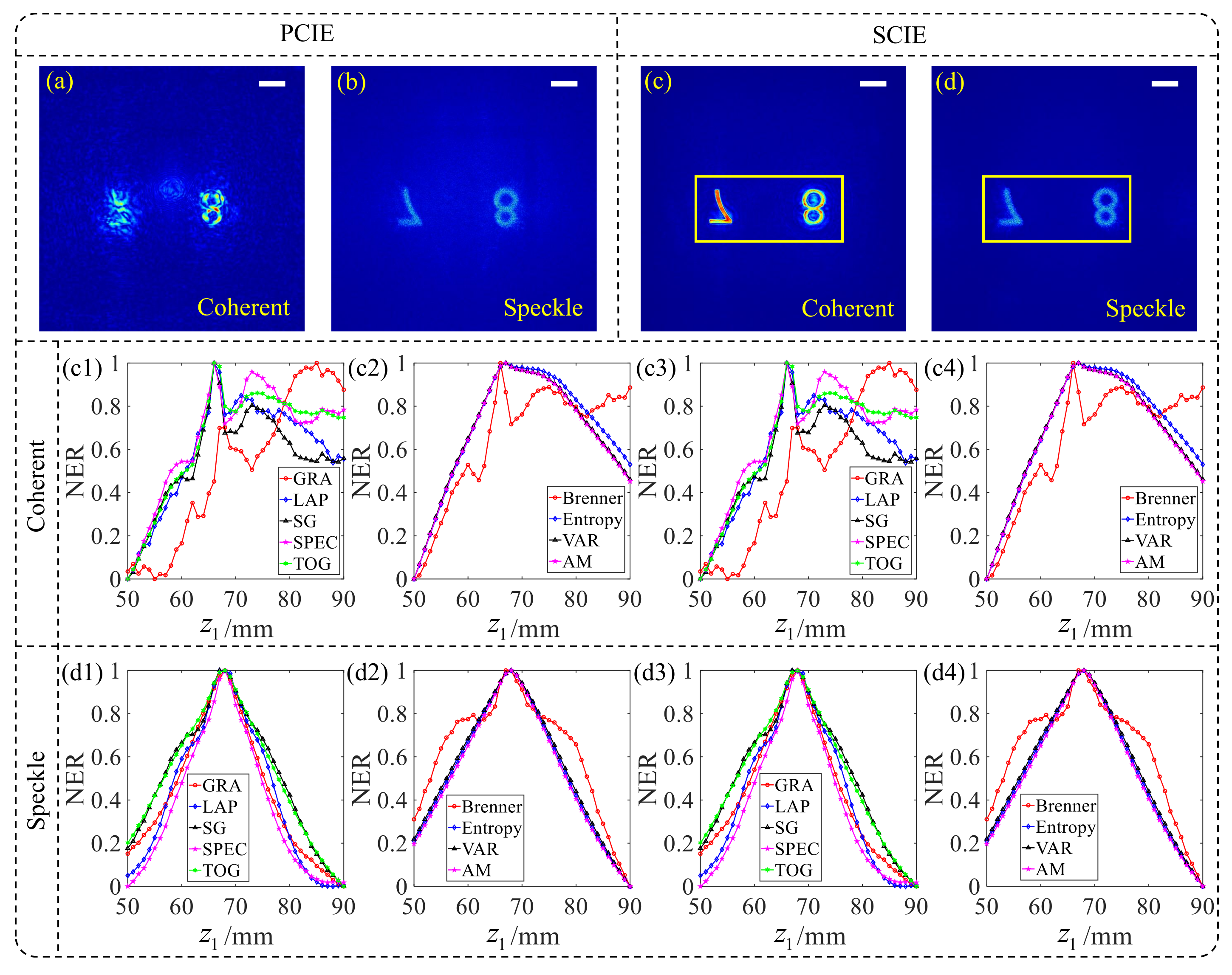
3.1. Comparison of the Two Iteration Methods

PCIE and SCIE are verified in the single-lens CDI system. The numerical simulations of convergence speed and robustness are presented in Figure 4, Figure 5 and Figure 6. The reconstructed images from PCIE and SCIE are shown in Figure 4a1–a4,b1–b4. The reconstructed result of SCIE is distinguishable and normalized correlation coefficient (NCC) reaches 1 after 100 iterations, whereas the result of PCIE is heavily degraded with the same iterations. SCIE performs well in the convergence speed compared to PCIE.
The robustness comparison of PCIE and SCIE is proved in Figure 5 [38]. A zero-mean Gaussian noise is added in all coherent patterns, and the variance of the noise is set as 0.01, 0.05, and 0.1, respectively. Figure 5a1–a3,b1–b3 show the reconstructed results under the noise of different variances by using PCIE and SCIE, respectively, after 1000 iterations. The reconstructed quality of SCIE is visually better than that of the PCIE with the same noise. The corresponding convergence curves are shown in Figure 5c. As the noise level increases, the reconstructed quality decreases for these two methods. NCC values of SCIE are always better than that of PCIE for different noise levels.
For the same condition as the previous set of simulations, Figure 6 shows the reconstructed results of the sample when the number of diffraction pattern is different. Figure 6a shows the ground truth. The speckle pattern incident on the sample is shown in Figure 6b. Figure 6a1–a8 are reconstructed results obtained by SCIE and PCIE, when the number of images is 3, 6, 9, and 11, respectively, by using diffraction patterns. Figure 6b1–b8 show this using speckle patterns. The NCC curves of PCIE and SCIE are plotted in Figure 6c1,c2 for coherent patterns and Figure 6d1,d2 are plotted for speckle patterns. The curves show that, regardless of the illumination mode, the convergence speed of SCIE is always better than PCIE. SCIE can converge after about 20 iterations, while PCIE convergence requires at least 50 iterations. SCIE achieves a good reconstruction from the results based on the simulation results above. SCIE is a better choice for reconstructing samples in the single-lens CDI system.
For a perfect sample reconstruction, object distance and image distance, according to z 1 and z 2 in Figure 1, are needed to be determined accurately. However, during the acquisition of the images, the distance of z 2 can be determined manually. The focus position is identified as the starting position of the recorded image. At this time, z 2 is the focal length of the lens L 2 in Figure 1. To verify the performance of the auto-focusing method proposed, the following two situations are considered.

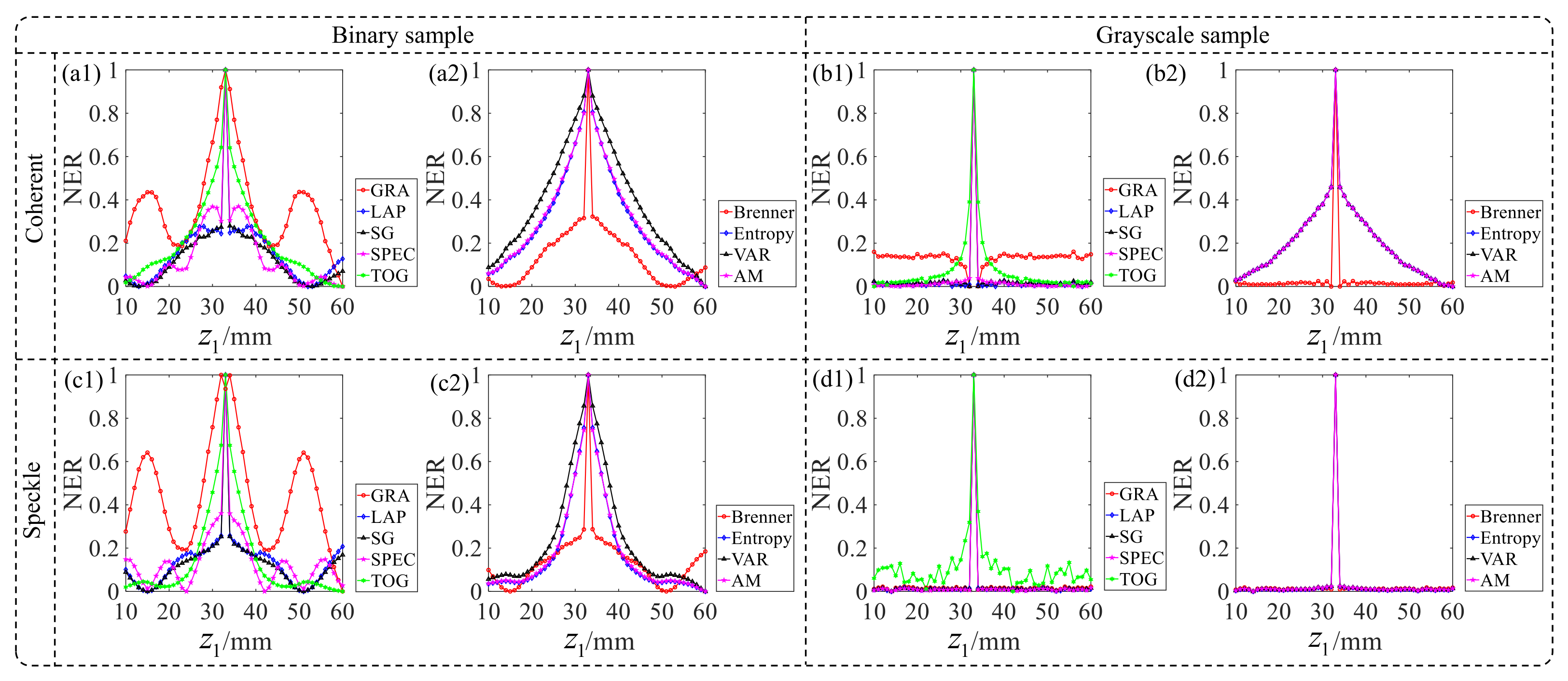
3.2. Autofocus for Object Distance

When only the object distance, z 1 in Figure 1, is unknown. The positive effect of the diffuser on estimating the distance value will be checked in the simulation. The search boundary of z 1 is 10 mm∼60 mm. To compare the results of CEFs in both coherent and speckle illumination, all evaluation results are normalized. The CEF curves are shown in Figure 7. Binary sample and grayscale sample used here correspond to Figure 4 and Figure 6a, respectively. The curves in Figure 7a1,a2,b1,b2 denote the results with the coherent illumination and the curves in the Figure 7c1,c2,d1,d2 are for the speckle illumination. For the binary sample, it is obvious that the speckle illumination is helpful for a stable and robust searching focus for all CEFs except GRA. The original correct result of GRA under coherent illumination is destroyed. The sensitivity of the curves is significantly improved. For the grayscale sample, the autofocus curves of the two illumination modes show good unimodality and high sensitivity, except for TOG. The curve performance of GRA, Entropy, and AM has been improved. However, the originally good TOG curve was destroyed. In summary, a diffuser is more conducive to accurately estimating the diffraction distance by CEFs. Speckle illumination is helpful for a unique and robust auto-focusing search even using the simple metric function in the single-lens CDI system.
The experimental verification is made by using the experimental device shown in Figure 8. A fiber laser (532 nm) is collimated by a lens (f = 200 mm). A diffuser (DG10-120-MD, Thorlabs, 120 grit) serves as a scattering medium. The focal length of lens L 2 is 35 mm. A CCD (3.1 μ m) is moved by a precision linear stage.
In the experiment, the sample is a calibration target engraved with ‘78’. The number of measured patterns is 11 and the interval is 1 mm. Figure 9a–d show the reconstructed results of SCIE and PCIE for the two illumination modes, respectively. Using diffraction patterns, the reconstructed results of PCIE are significantly better than that of SCIE. Even though the reconstructed image in Figure 9c has the twin-image effect and some noise around digits, Figure 9a shows the result of unsuccessful reconstruction after 1000 iterations. For the reconstructed results by using speckle patterns, the reconstructed results of PCIE and SCIE can both distinguish the number ‘78’, in Figure 9b,d, respectively. The reconstructed result of SCIE has higher contrast visually. Figure 9c1–c4,d1–d4 show the CEF curves for coherent and speckle illumination, respectively. Speckle illumination optimizes the large fluctuating CEF curves under coherent illumination. We cropped the information-rich area in the reconstructed image data set corresponding to the yellow box in Figure 9c,d. The clarity of this area is evaluated, and the corresponding CEF curves are shown in Figure 9c3,c4,d3,d4. When evaluating the clarity of the rich-information area of the image, speckle illumination still shows superiority. Therefore, speckle illumination plays a positive role in single-lens CDI object distance scanning, which not only makes the SQF curve unimodal but also improves the accuracy of the auto-focusing results.
The diffuser provides random illumination for the imaging system, which will disorganize the tilt phase factor and counteract the lateral shift effect of intensity pattern. This property is called the memory effect of speckle [39,40]. The speckle pattern is inherently random, so oblique illumination will not affect it. Furthermore, speckle illumination can eliminate the aliasing artifact and enhance the robustness [32].

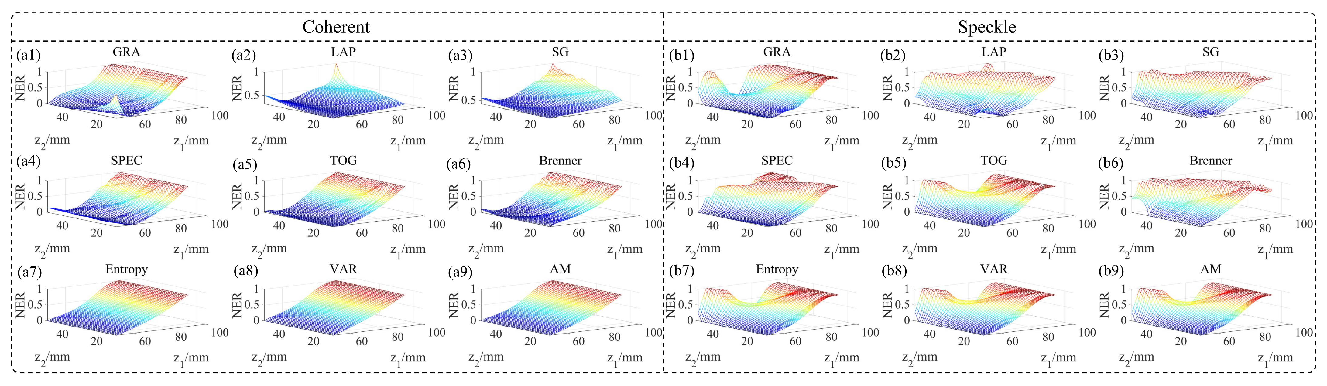
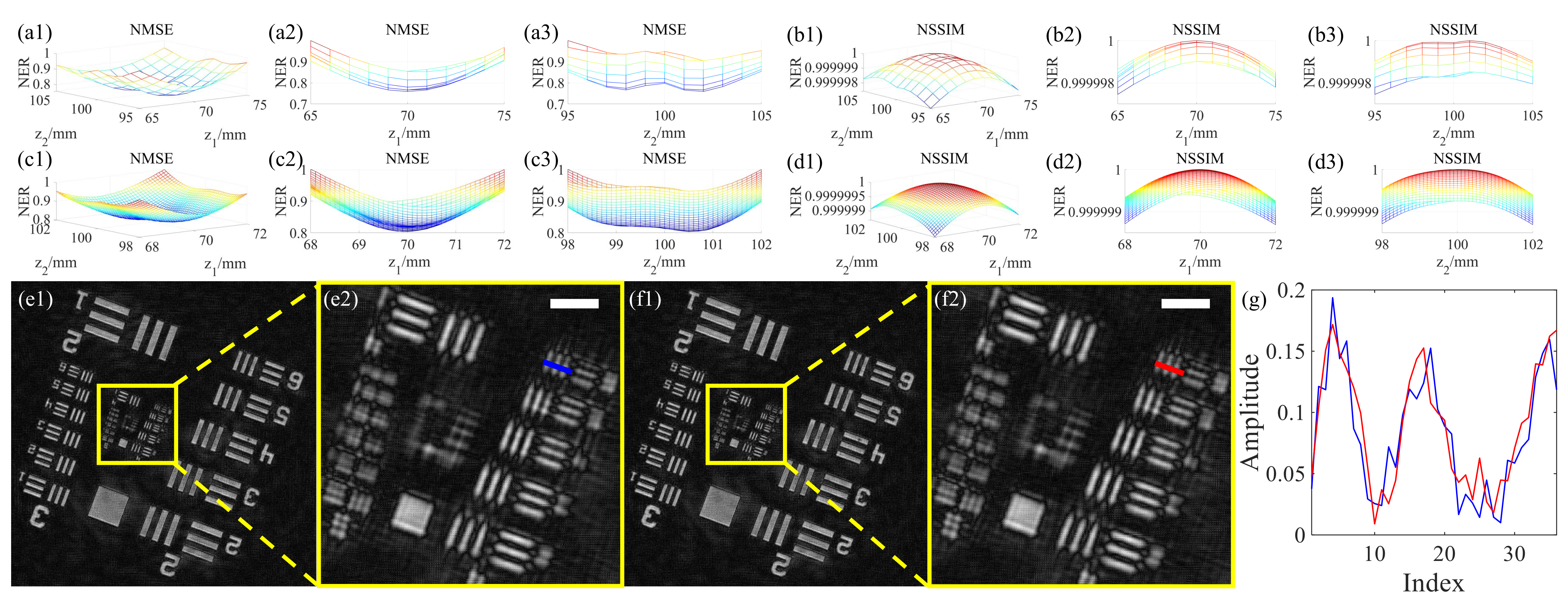
3.3. Autofocus for Object Distance and Image Distance

The other case in the single-lens CDI we consider is two-unknown-distance autofocus, the object distance, and image distance. In Section 3.2, speckle illumination played a positive role in one-unknown-distance autofocus. We expect it to work for autofocus in two-unknown-distance autofocus. Then we test the experimental data set ‘78’. Based on the distance obtained in Figure 9, we reset the object distance scanning boundary 50 mm∼90 mm, the image distance scanning range from 15 mm∼55 mm, and the step length is 1 mm. The results are shown in Figure 10a1–a9,b1–b9. In a large range and long step length autofocus, neither coherent illumination nor speckle illumination can give a rough focus trend. Therefore, in the single-lens CDI, when the object and image distances are auto-focusing scanned simultaneously, the diffuser makes no sense.
Therefore, for single-lens CDI dual-distance autofocus, a new focus strategy is proposed. Usually, MSE and SSIM are used to detect the effect of image retrieval in simulation [41,42,43,44,45] and the reference value of the function is the ground truth. In the experiment, the ground truth of the sample is unavailable. Therefore, the pixel average is selected as the reference value here. Their expressions are as follows
MSE U S n , I r e f = 1 M n = 1 N U S n I r e f 2 ,
where U S n has been defined in Equation (14), M represents the number of pixels and I r e f is the pixel mean of the U S n , its data set is written as
I r e f = 1 n n = 1 N U S n .
Here the structural similarity (SSIM) function is shown as
SSIM U S n , I r e f = 2 μ U S n μ I r e f + c 1 μ U S n 2 + μ I r e f 2 + c 1 2 σ U S n I r e f + c 2 σ U S n 2 + σ I r e f 2 + c 2 ,
where μ U S n is pixel mean value of image U S n , μ I r e f is pixel mean value of image I r e f . σ U S n 2 and σ I r e f 2 are the variances of images U S n and μ I r e f . σ U S n I r e f represents the covariance of the two images. c 1 = ( k 1 L ) 2 and c 2 = ( k 2 L ) 2 are constants used to maintain stability. L is the dynamic range of pixel values. Generally k 1 = 0.01 , k 2 = 0.03 .
A negative 1951 USAF target (R3L3S1N, Thorlabs) is used as the sample and the focal distance is 100 mm. The results of MSE and SSIM are normalized. Figure 11a1–a3,b1–b3 show the rough auto-focusing curves of NMSE and NSSIM with the search boundary of 65 mm∼75 mm and 95 mm∼105 mm, the step is 1 mm. The highest peak can be identified in the CEF curves of z 2 , but not unimodal by using NMSE and NSSIM. We refine the search interval to 0.01 mm with the same search boundary. Figure 11c1–c3,d1–d3 show the fine auto-focusing curves. The results obtained by NMSE are z 1 = 69.9 mm, z 2 = 100.5 mm while the results of NSSIM are z 1 = 70 mm, z 2 = 100 mm. As for the CEF curves, z 2 of NMSE steal has two peaks, NSSIM shows 2D unimodal.
The retrieved sample with the above two sets of auto-focusing results is shown in Figure 11e1,e2,f1,f2. Figure 11e2,f2 correspond to the content of the yellow area in Figure 11e1,f1, respectively. Figure 11g corresponds to the pixel information of the red and blue lines in Figure 11e2,f2, respectively. The line drawing position is the sixth line pair of the fourth group of the resolution board. The image resolution retrieved based on the auto-focusing results of NMSE and NSSIM are almost the same. MSE and NSSIM can realize automatic focusing at the same time as the object distance and the image distance in single-lens CDI. SSIM shows its superiority in focusing accuracy.

4. Conclusions

In this work, we insert a diffuser into the single-lens CDI system to improve the accuracy and robustness of the autofocus algorithm. Our proposed SCIE algorithm can reconstruct samples with fast iteration speed and robustness in a single-lens CDI. We proposed the use of NMSE and NSSIM in two-unknown-distance autofocusing with taking the pixel mean value of the reconstructed image data set as the reference input. The 2D CEF curves show good unimodality. This paper provides new strategies for reconstruction samples and auto-focusing in the single-lens imaging system, which provides imaging solutions for CDI systems with a lens.

Author Contributions

Experiments, methodology and writing, X.Z.; investigation, X.W.; visualization, Y.J.; investigation, Y.L.; review and editing, S.L.; review, editing and supervision, Z.L. All authors have read and agreed to the published version of the manuscript.

Funding

National Natural Science Foundation of China (11874132, 61975044, 12074094); Interdisciplinary Research Foundation of HIT (IR2021237).

Institutional Review Board Statement

Not applicable.

Informed Consent Statement

Not applicable.

Data Availability Statement

Data underlying the results presented in this paper are not publicly available at this time but may be obtained from the authors upon reasonable request.

Acknowledgments

The authors would like to thank Miguel Victor for his writing advice, Cheng Guo for his experimental and methodological guidance, and Yong Geng and Jiaxin Wang for their suggestions on the revision of the article. The authors would also like to thank the editors and the three reviewers who made valuable comments that helped us improve this paper.

Conflicts of Interest

The authors declare no conflict of interest.

References

  1. Fienup, J.R. Phase retrieval algorithms: A comparison. Appl. Opt. 1982, 21, 2758–2769. [Google Scholar] [CrossRef] [PubMed] [Green Version]
  2. Li, F.X.; Yan, W.; Peng, F.P.; Wang, S.M.; Du, J.L. Enhanced phase retrieval method based on random phase modulation. Appl. Sci. 2020, 10, 1184. [Google Scholar] [CrossRef] [Green Version]
  3. Xu, Y.S.; Ye, Q.; Hoorfar, A.; Meng, G.X. Extrapolative phase retrieval based on a hybrid of PhaseCut and alternating projection techniques. Opt. Lasers Eng. 2019, 121, 96–103. [Google Scholar] [CrossRef]
  4. Shan, M.G.; Liu, L.; Zhong, Z.; Liu, B.; Zhang, Y.B. Direct phase retrieval for simultaneous dual-wavelength off-axis digital holography. Opt. Lasers Eng. 2019, 121, 246–251. [Google Scholar] [CrossRef]
  5. Sun, M.J.; Zhang, J.M. Phase retrieval utilizing geometric average and stochastic perturbation. Opt. Lasers Eng. 2019, 120, 1–5. [Google Scholar] [CrossRef]
  6. Tsuruta, M.; Fukuyama, T.; Tahara, T.; Takaki, Y. Fast image reconstruction technique for parallel phase-shifting digital holography. Appl. Sci. 2021, 11, 11343. [Google Scholar] [CrossRef]
  7. Guo, C.; Shen, C.; Tan, J.B.; Bao, X.J.; Liu, S.T.; Liu, Z.J. A robust multi-image phase retrieval. Opt. Lasers Eng. 2018, 101, 16–22. [Google Scholar] [CrossRef]
  8. Bao, P.; Zhang, F.C.; Pedrini, G.; Osten, W. Phase retrieval using multiple illumination wavelengths. Opt. Lett. 2008, 33, 309–311. [Google Scholar] [CrossRef]
  9. Kühn, J.; Colomb, T.; Montfort, F.; Charrière, F.; Emery, Y.; Cuche, E.; Marquet, P.; Depeursinge, C. Real-time dual-wavelength digital holographic microscopy with a single hologram acquisition. Opt. Express 2007, 15, 7231–7242. [Google Scholar] [CrossRef]
  10. Pedrini, G.; Osten, W.; Zhang, Y. Wave-front reconstruction from a sequence of interferograms recorded at different planes. Opt. Lett. 2005, 30, 833–835. [Google Scholar] [CrossRef]
  11. Geng, Y.; Tan, J.B.; Guo, C.; Shen, C.; Ding, W.Q.; Liu, S.T.; Liu, Z.J. Computational coherent imaging by rotating a cylindrical lens. Opt. Express 2018, 26, 22110–22122. [Google Scholar] [CrossRef] [PubMed]
  12. Shen, C.; Guo, C.; Geng, Y.; Tan, J.B.; Liu, S.T.; Liu, Z.J. Noise-robust pixel-super-resolved multi-image phase retrieval with coherent illumination. J. Opt. 2018, 20, 115703. [Google Scholar] [CrossRef]
  13. Guo, C.; Li, Q.; Tan, J.B.; Liu, S.T.; Liu, Z.J. A method of solving tilt illumination for multiple distance phase retrieval. Opt. Lasers Eng. 2018, 106, 17–23. [Google Scholar] [CrossRef]
  14. Guo, C.; Zhao, Y.X.; Tan, J.B.; Liu, S.T.; Liu, Z.J. Multi-distance phase retrieval with a weighted shrink-wrap constraint. Opt. Lasers Eng. 2019, 113, 1–5. [Google Scholar] [CrossRef]
  15. Luo, W.; Zhang, Y.; Feizi, A.; Göröcs, Z.; Ozcan, A. Pixel super-resolution using wavelength scanning. Light Sci. Appl. 2016, 5, e16060. [Google Scholar] [CrossRef] [Green Version]
  16. Liu, Z.J.; Guo, C.; Tan, J.B.; Wu, Q.; Pan, L.Q.; Liu, S.T. Iterative phase-amplitude retrieval with multiple intensity images at output plane of gyrator transforms. J. Opt. 2015, 17, 025701. [Google Scholar] [CrossRef]
  17. Jin, X.; Ding, X.M.; Tan, J.B.; Shen, C.; Liu, S.T.; Liu, Z.J. Wavefront reconstruction of a non-coaxial diffraction model in a lens system. Appl. Opt. 2018, 57, 1127–1133. [Google Scholar] [CrossRef]
  18. Shen, C.; Tan, J.B.; Wei, C.; Liu, Z.J. Coherent diffraction imaging by moving a lens. Opt. Express 2016, 24, 16520–16529. [Google Scholar] [CrossRef]
  19. Almoro, P.F.; Gundu, P.N.; Hanson, S.G. Numerical correction of aberrations via phase retrieval with speckle illumination. Opt. Lett. 2009, 34, 521–523. [Google Scholar] [CrossRef]
  20. Zhu, F.P.; Lu, R.Z.; Bai, P.X.; Lei, D. A novel in situ calibration of object distance of an imaging lens based on optical refraction and two-dimensional DIC. Opt. Lasers Eng. 2019, 120, 110–117. [Google Scholar] [CrossRef]
  21. Wang, X.Z.; Liu, L.; Du, X.H.; Zhang, J.; Ni, G.M.; Liu, J.X. GMANet: Gradient mask attention network for finding clearest human fecal microscopic image in autofocus process. Appl. Sci. 2021, 11, 10293. [Google Scholar] [CrossRef]
  22. Yang, C.P.; Chen, M.H.; Zhou, F.F.; Li, W.; Peng, Z.M. Accurate and rapid auto-focus methods based on image quality assessment for telescope observation. Appl. Sci. 2020, 10, 658. [Google Scholar] [CrossRef] [Green Version]
  23. Zhang, Y.B.; Wang, H.D.; Wu, Y.C.; Tammamitsu, M.; Ozcan, A. Edge sparsity criterion for robust holographic autofocusing. Opt. Lett. 2017, 42, 3824–3827. [Google Scholar] [CrossRef] [PubMed]
  24. Sun, Y.; Duthaler, S.; Nelson, B.J. Autofocusing algorithm selection in computer microscopy. In Proceedings of the 2005 IEEE RSJ International Conference on Intelligent Robots Systems, Edmonton, Alta, 2–6 August 2005; pp. 70–76. [Google Scholar]
  25. Santos, A.; Solórzano, C.O.; Vaquero, J.J.; Peña, J.M.; Malpica, N.; Pozo, F. Evaluation of autofocus functions in molecular cytogenetic analysis. J. Microsc. 1997, 188, 264–272. [Google Scholar] [CrossRef] [Green Version]
  26. Brenner, J.F.; Dew, B.S.; Horton, J.B.; King, J.B.; Neirath, P.W.; Sellers, W.D. An automated microscope for cytologic research a preliminary evaluation. J. Histochem. Cytochem. 1976, 24, 100–111. [Google Scholar] [CrossRef] [PubMed]
  27. Yeo, T.T.E.; Ong, S.H.; Sinniah, R. Autofocusing for tissue microscopy. Image Vision Comput. 1993, 11, 629–639. [Google Scholar] [CrossRef]
  28. Dwivedi, P.; Konijnenberg, A.P.; Pereira, S.F.; Urbach, H.P. Lateral position correction in ptychography using the gradient of intensity patterns. Ultramicroscopy 2018, 192, 29–36. [Google Scholar] [CrossRef]
  29. Langehanenberg, P.; Kemper, B.; Dirksen, D.; Bally, G.V. Autofocusing in digital holographic phase contrast microscopy on pure phase objects for live cell imaging. Appl. Opt. 2008, 47, D176–D182. [Google Scholar] [CrossRef] [PubMed]
  30. Vollath, D. The influence of the scene parameters and of noise on the behavior of automatic focusing algorithms. J. Microsc. 1988, 151, 133–146. [Google Scholar] [CrossRef]
  31. Shenfield, A.; Rodenburg, J.M. Evolutionary determination of experimental parameters for ptychographical imaging. J. Appl. Phys. 2011, 109, 124510. [Google Scholar] [CrossRef] [Green Version]
  32. Guo, C.; Zhao, Y.X.; Tan, J.B.; Liu, S.T.; Liu, Z.J. Adaptive lens-free computational coherent imaging using autofocusing quantification with speckle illumination. Opt. Express 2018, 26, 14407–14420. [Google Scholar] [CrossRef] [PubMed]
  33. Yazdanfar, S.; Kenny, K.B.; Tasimi, K.; Corwin, A.D.; Dixon, E.L.; Filkins, R.J. Simple and robust image-based autofocusing for digital microscopy. Opt. Express 2008, 12, 8670–8677. [Google Scholar] [CrossRef] [PubMed]
  34. Sun, Y.; Duthaler, S.; Nelson, B.J. Autofocusing in computer microscopy: Selecting the optimal focus algorithm. Microsc. Res. Techniq. 2004, 65, 139–149. [Google Scholar] [CrossRef] [PubMed]
  35. Choi, Y.S.; Lee, S.J. Three-dimensional volumetric measurement of red blood cell motion using digital holographic microscopy. Appl. Opt. 2009, 48, 2983–2990. [Google Scholar] [CrossRef]
  36. Yang, Y.; Kang, B.S.; Choo, Y.J. Application of the correlation coefficient method for determination of the focal plane to digital particle holography. Appl. Opt. 2008, 47, 817–824. [Google Scholar] [CrossRef] [Green Version]
  37. Goodman, J.W. Introduction to Fourier Optics, 3rd ed.; Roberts and Company Publishers: Greenwood Village, CO, USA, 2004; pp. 154–162. [Google Scholar]
  38. Hardin. Centers for Disease Control and Prevention. Available online: https://phil.cdc.gov/Details.aspx?pid=22920 (accessed on 25 October 2021).
  39. Freund, I.; Rosenbluh, M.; Feng, S.C. Memory effects in propagation of optical waves through disordered media. Phys. Rev. Lett. 1988, 61, 2328–2331. [Google Scholar] [CrossRef]
  40. Bertolotti, J. Multiple scattering: Unravelling the tangle. Nat. Phys. 2015, 11, 622–623. [Google Scholar] [CrossRef]
  41. Wen, X.; Geng, Y.; Guo, C.; Zhou, X.Y.; Tan, J.B.; Liu, S.T.; Tan, C.M.; Liu, Z.J. A parallel ptychographic iterative engine with a co-start region. J. Opt. 2020, 22, 1–11. [Google Scholar] [CrossRef]
  42. Wen, X.; Geng, Y.; Zhou, X.Y.; Tan, J.B.; Liu, S.T.; Tan, C.M.; Liu, Z.J. Ptychography imaging by 1-D scanning with a diffuser. Opt. Express 2020, 28, 22658–22668. [Google Scholar] [CrossRef]
  43. Zhang, F.L.; Guo, C.; Zhai, Y.L.; Tan, J.B.; Liu, S.T.; Tan, C.M.; Chen, H.; Liu, Z.J. A noise-robust multi-intensity phase retrieval method based on structural patch decomposition. J. Opt. 2020, 22, 075706. [Google Scholar] [CrossRef]
  44. Qin, Y.; Wang, Z.P.; Wang, H.J.; Gong, Q.; Zhou, N.R. Robust information encryption diffractive-imaging-based scheme with special phase retrieval algorithm for a customized data container. Opt. Lasers Eng. 2018, 105, 118–124. [Google Scholar] [CrossRef]
  45. Wang, Z.; Bovik, A.C.; Sheikh, H.R.; Simoncelli, E.P. Image quality assessment: From error visibility to structural similarity. IEEE Trans. Image Process. 2004, 13, 600–612. [Google Scholar] [CrossRef] [PubMed] [Green Version]
Figure 1. An optical setup for single-lens CDI with coherent and speckle illumination. AS: aperture stop; L 1 , L 2 : lens; D: diffuser; S: sample; SP: sensor plane.
Applsci 12 01378 g001
Figure 2. The flowchart of autofocus and image reconstruction in single-lens CDI.
Applsci 12 01378 g002
Figure 3. The flowchart of CIE. SL: single lens.
Applsci 12 01378 g003
Figure 4. Reconstructed results of PCIE and SCIE. (a1a4) and (b1b4) are reconstructed images; (c) is the logarithm of mean square error (LMSE) curves of the reconstruction results from the two modes.
Applsci 12 01378 g004
Figure 5. Noise robustness of PCIE and SCIE. (a1a3) the reconstructed images with the variance of 0.01, 0.05, and 0.1 for PCIE; (b1b3) the reconstructed images with the variance of 0.01, 0.05 and 0.1 for SCIE; (c) NCC curves.
Applsci 12 01378 g005
Figure 6. Diffraction and speckle reconstructed results with different numbers of images and NCC curves. (a), the ground truth; (b), the speckle pattern; (a1a8) are reconstructed images obtained by PCIE and SCIE, respectively, by using diffraction patterns, when the number of images is 3, 6, 9 and 11. (b1b8) are reconstructed images using speckle patterns in the same case. (c1,c2,d1,d2) are the corresponding NCC curves. Digits represent the number of patterns, P, pattern.
Applsci 12 01378 g006
Figure 7. The performance of autofocus by coherent illumination and speckle illumination, respectively: (a1,a2,b1,b2) show the CEF curves of binary and grayscale sample respectively by using diffraction patterns; (c1,c2,d1,d2) show the CEF curves of binary and grayscale sample respectively by using speckle patterns.
Applsci 12 01378 g007
Figure 8. The schematic diagram of the CDI setup.
Applsci 12 01378 g008
Figure 9. The reconstructed results and normalized CEF curves. (ad) are the reconstructed results; (c1c4) are the CEF curves for diffraction patterns; (d1d4) are the CEF curves for speckle patterns. NER: normalized evaluation result. The white bar corresponds to 620 μ m.
Applsci 12 01378 g009
Figure 10. CEFs experimental results of simultaneous scanning of object and image distances: (a1a9) display the CEF curves under coherent illumination; (b1b9) display the CEF curves under speckle illumination.
Applsci 12 01378 g010
Figure 11. Auto-focusing curves and sample reconstruction results. (a1a3) and (b1b3) are the rough auto-focusing curves of NMSE and NSSIM, respectively; (c1c3) and (d1d3) are the fine auto-focusing curves of NMSE and NSSIM, respectively; (e1,e2,f1,f2) are the reconstruction results using the quasi-focal distances from (c1,d1), respectively; (g) pixel contrast curves. The white bar corresponds to 200 μ m.
Applsci 12 01378 g011
Publisher’s Note: MDPI stays neutral with regard to jurisdictional claims in published maps and institutional affiliations.

