Article

An Advanced AFWMF Model for Identifying High Random-Valued Impulse Noise for Image Processing

1
Department of Electronic Engineering, National Ilan University, Yilan City 26047, Taiwan
2
Department of Information Management, Hwa Hsia University of Technology, New Taipei City 23568, Taiwan
3
Department of Digital Multimedia Design, National Taipei University of Business, Taipei City 100025, Taiwan
*
Authors to whom correspondence should be addressed.
Appl. Sci. 2021, 11(15), 7037; https://doi.org/10.3390/app11157037
Submission received: 28 June 2021 / Revised: 26 July 2021 / Accepted: 27 July 2021 / Published: 30 July 2021
(This article belongs to the Special Issue Advances in Digital Image Processing)

Abstract

:
In this study, a novel adaptive fuzzy weighted mean filter (AFWMF) model based on the directional median technique and fuzzy inference is presented for solving the restoring high-ratio random-valued noise in image processing. This study aims, not only to obtain information from each direction of the filtering window, but also to gain information from every pixel of the filtering windows completely. Thus, in order to implement preserving details and textures for better restoration in high-noise cases, this study utilizes the directional median to build the membership function in fuzzy inference dynamically, then calculates the weighted window corresponding to the filtering window using fuzzy inference to represent the importance of valuable pixels. Finally, the restoration pixel is calculated using the weighted window and the filtering window for the weighted mean. Subsequently, this new AFWMF model significantly improves performances in the measurement of the peak signal to noise ratio (PSNR) value for preserving detail and fixed image in noise density within the range of 20–70% for the five well-known experimental images. In extensive experiments, this study also shows the better performance of identifying the proposed peak signal-to-removal noise ratio (PSRNR) and evaluating psycho-visual tests than other listed filter methods. Furthermore, the proposed AFWMF model also has a better structural similarity index measure (SSIM) value of another indicator. Conclusively, two interesting and meaning findings are identified: (1) the proposed AFWMF model is generally the best model among the 10 listed filtering methods for image processing in terms of the measurement of two quantitative indicators for both the PSNR and SSIM values; (2) different impulse noise densities should be made for different filtering methods, and thus, this is an important and interesting issue when aiming to identify an appropriate filtering model from a variety of images for processing various noise densities.

1. Introduction

Impulse noise frequently contaminates digital photographs. A sensor or a noisy transmission medium can pollute the source, making it inaccurate [1,2]. When an image is polluted, this means that some parts of the image are replaced by impulse noise [3,4]. There are two forms of noise in general. One form of noise is known as salt and pepper noise. It has a fixed value at both ends of the gray scale. In 8-bit grayscale, pixels contain noise values of 0 and 255. Another type is called uniform impulse noise or random-valued impulse noise. This noise will disperse its pixel values from 0 to 255 equally [5]. There have been several techniques used for removing salt and pepper noise, and some of them have proven to be effective [6,7,8,9]. However, many academic researchers are still interested in developing a random-valued impulse filter.
Many spatial filters have been developed for removing impulse noise. The most powerful spatial filter is the median filter [1,10,11]. By using this filter, we can remove the impulse noise from random values. The median filter replaces the filtering window’s centered pixels with the filtering window’s median. This filter applies a median operation for every pixel. Therefore, it modifies both undisturbed pixels and pixels with noise, and some detail which must be preserved in an image is removed [1]. Some modified median filters, such as the weighted median filter [12] and the center-weighted median filter [13], have been implemented to solve this problem. These two filters can operate effectively at low noise ratios but not at high noise ratios, since their performance in terms of spurious and missing detections is constrained [12]. This is resolved by using a switching median filter [13,14]. This filter is mainly used for noise median filtering and detection mechanisms. A threshold is used in the detection stage to detect whether the data are tainted [12]. The filtering process is executed only if the filter contains noise.
Later, various methods for reducing random-valued impulse noise were devised, such as the tri-state median filter [15], the directional weighted median filter [16], the modified switching median filter [17], the fuzzy-reasoning median filter [18], the simple adaptive median filter [19], the efficient decision-based algorithm [20], neural networks and fuzzy decisions [21], the elimination of impulse noise using an efficient algorithm [22], and threshold Boolean filtering [23], but these methods can fail at noise ratios over than 50 percent when using ranking order absolute difference [3,4] and adaptive switching median filters [12]. The above filters apply the standard median filter at the filtering stage. In general, the median filter could be poor when used with high noise ratios of over 50%. As a result, the adaptive fuzzy weighted mean filter (AFWMF) model is proposed to be used in this study for reducing and overcoming this problem, as it does not rely primarily on the median operation to replace noise.
The AFWMF model uses a directional median to preserve detail and calculate the weights of pixels in the filtering window with fuzzy rules. Each weight is represented as a pixel, which should provide useful information for restoration to enhance filtering performance. Fuzzy inference membership functions can change dynamically depending on the distribution of the filter window to manage random-valued impulse noise. As a result, it is expected that the AFWMF model will enhance filtering performance. In addition, the detection of the switching framework will affect the filter stage of the same framework directly. Therefore, this study modifies the ROR (robust outlyingness ratio) detection algorithm, using fuzzy rules to make the ROR algorithm more precise and powerful.
This study is structured in the following order. Section 2 reviews the ROR detection algorithm and filter order. Section 3 introduces the AFWMF model in detail. Section 4 summarizes the proposed algorithm of the AFWMF model. Section 5 contains the empirical results obtained, illustrating the accuracy of the novel method using multiple testing photos. Finally, conclusions are drawn in Section 5.

2. Related Work

This section reviewed some related works in this study, including filtering windows and tag windows, robust outlyingness ratio, sparsity ranking, and noise models.

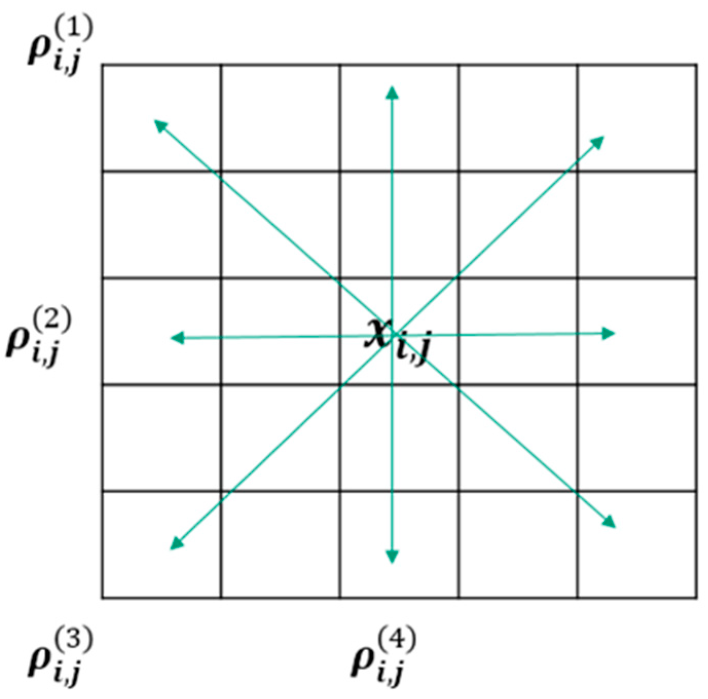
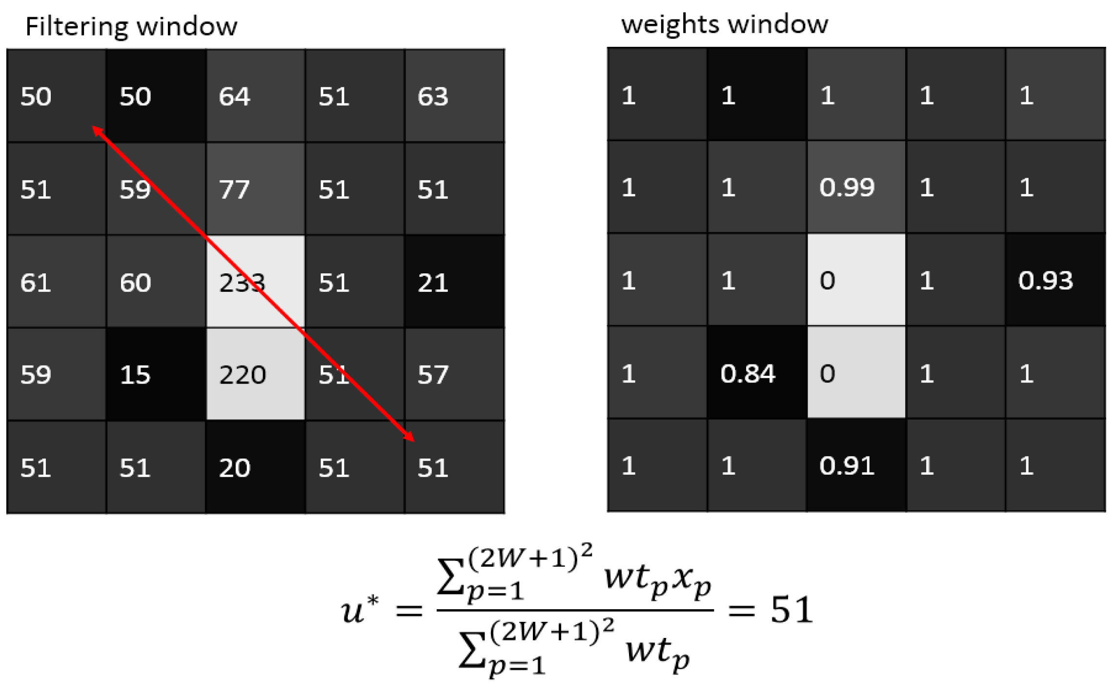
2.1. Filtering Window and Tag Window

For handling our proposed method, a filtering window and a tag window were defined as follows. A matrix X with the size (R × C ) was built for the input image. The filtering window was a square matrix. It had odd ( 2 W + 1 ) × ( 2 W + 1 ) dimensions. It is represented as follows:
X i , j = { x s , t | i W s i + W ,   j W t j + W } ,
where 1 i R , 1 j C , W 1 .
The corresponding binary tag matrix F is the same size as X . The sub matrix of F is called tag window F i , j ; its central pixel is at location ( i , j ) , the same as X i , j on the image, and it is formatted as:
F i , j = { f s , t | i W s i + W ,   j W t j + W } ,
When x s , t in Equation (1) was detected as a noisy pixel, f s , t in Equation (2) was set to one; when x s , t was not detected as a noisy pixel, f s , t was set to zero.

2.2. Robust Outlyingness Ratio
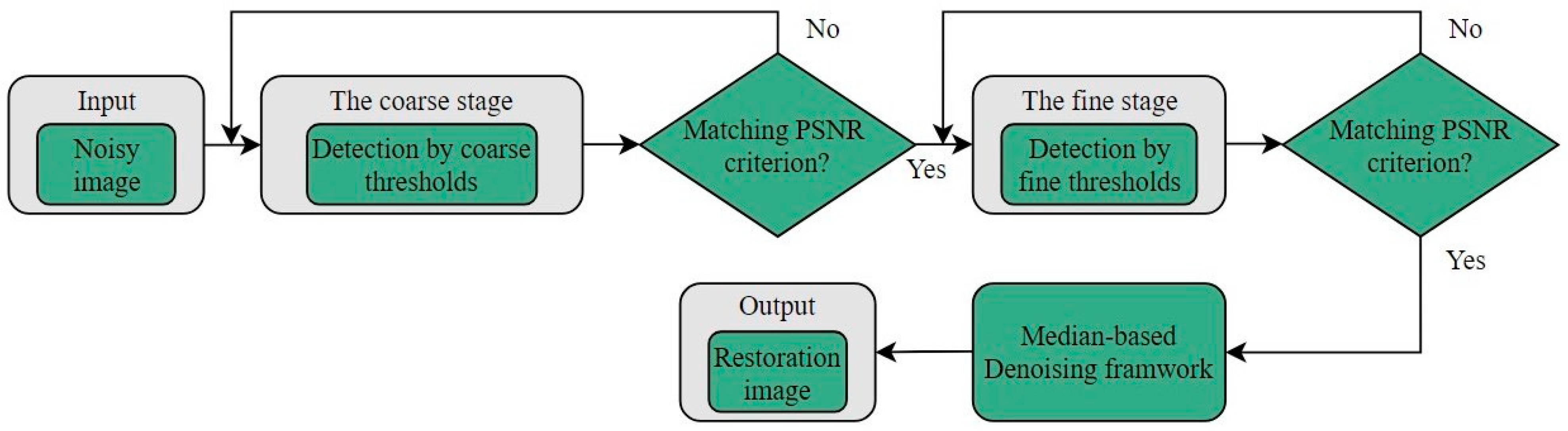
In order to be more robust and effective, we used a type of coarse-to-fine strategy based on the iterative framework for detecting random-valued impulse noise [12,16,24,25,26]. We used ROR to estimate whether the current pixel was a noise or not [16]. We briefly reviewed this algorithm as follows:
  • Coarse stage:
    1.
    Let us consider parameters J C = 1 and T c 1 ,   T c 2 ,   T c 3 as coarse thresholds. We initialized all of them with zeros in the tag matrix.
    2.
    For every pixel in the image, we found its ROR; if it ranged in the fourth level, as shown in Table 1, then that pixel was noise-free. We set the tag to 1; else, we found the relative divergence d among the filtering window’s median and active pixels. Then, based on the ROR value of d, we compared it to T c k . We checked whether it was noisy or noise-free. We checked if d was bigger than T c k . According to the r, we updated the tag matrix.
    3.
    If J c m c ,   J c = J c + 1 , then we repeated Step 2; else, this stage was completed.
  • Fine stage:
    1.
    Let us consider parameters J f = 1   and   T f 1 ,   T f 2 ,   T f 3 ,   T f 4 as fine thresholds. We initialized all of them with zeros in the tag matrix.
    2.
    For every pixel in the image, we found its ROR; if it ranged in fourth level, as shown in Table 1, then that pixel was noise-free. We set the tag to 1, or else found the relative divergence d among the filtering window’s median and active pixel. Then, based on the ROR value of d, we compared it to T f k . We checked whether it was noisy or noise-free. We checked if d was bigger than T f k . According to the r, we updated the tag matrix. Similarly, we calculated the values for all the pixels.
    3.
    If J f m f ,   J f = J f + 1 , then we repeated Step 2; else, this stage was completed.
m c and m f are shown in Table 2.
For the ROR algorithm, the operation was carried out in two stages—i.e., detection followed by filtering. For detection, first the ROR was measured to find the impulse of each pixel; then, all the pixels were divided into four levels according to their ROR values. Second, different decision rules were used to detect the impulse noise based on the absolute deviation from the median in each cluster. In order to make the detection results more accurate and robust, the from-coarse-to-fine strategy and the iterative framework were used for filtering. The structural flowchart of ROR is shown in Figure 1.

2.3. Sparsity Ranking
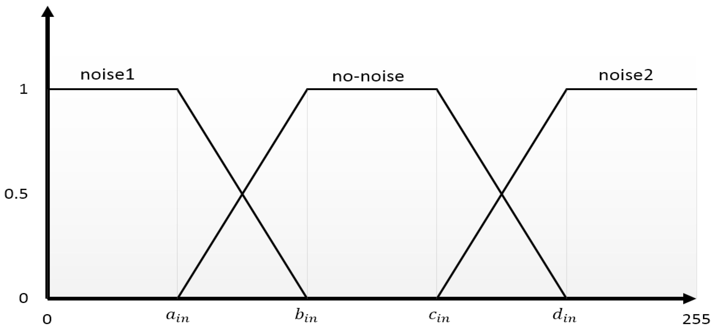
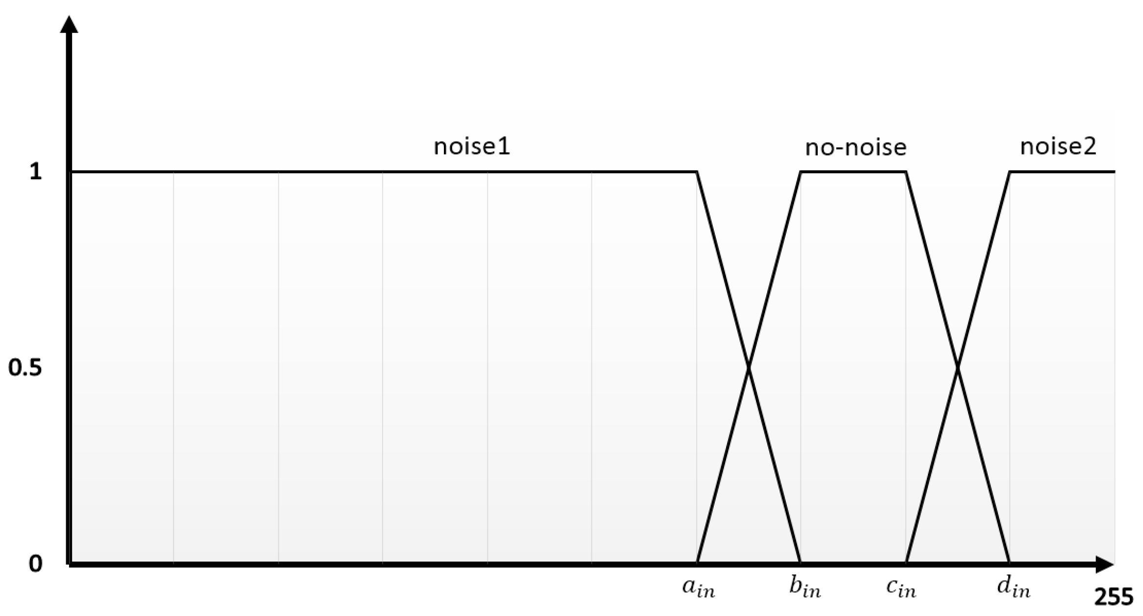
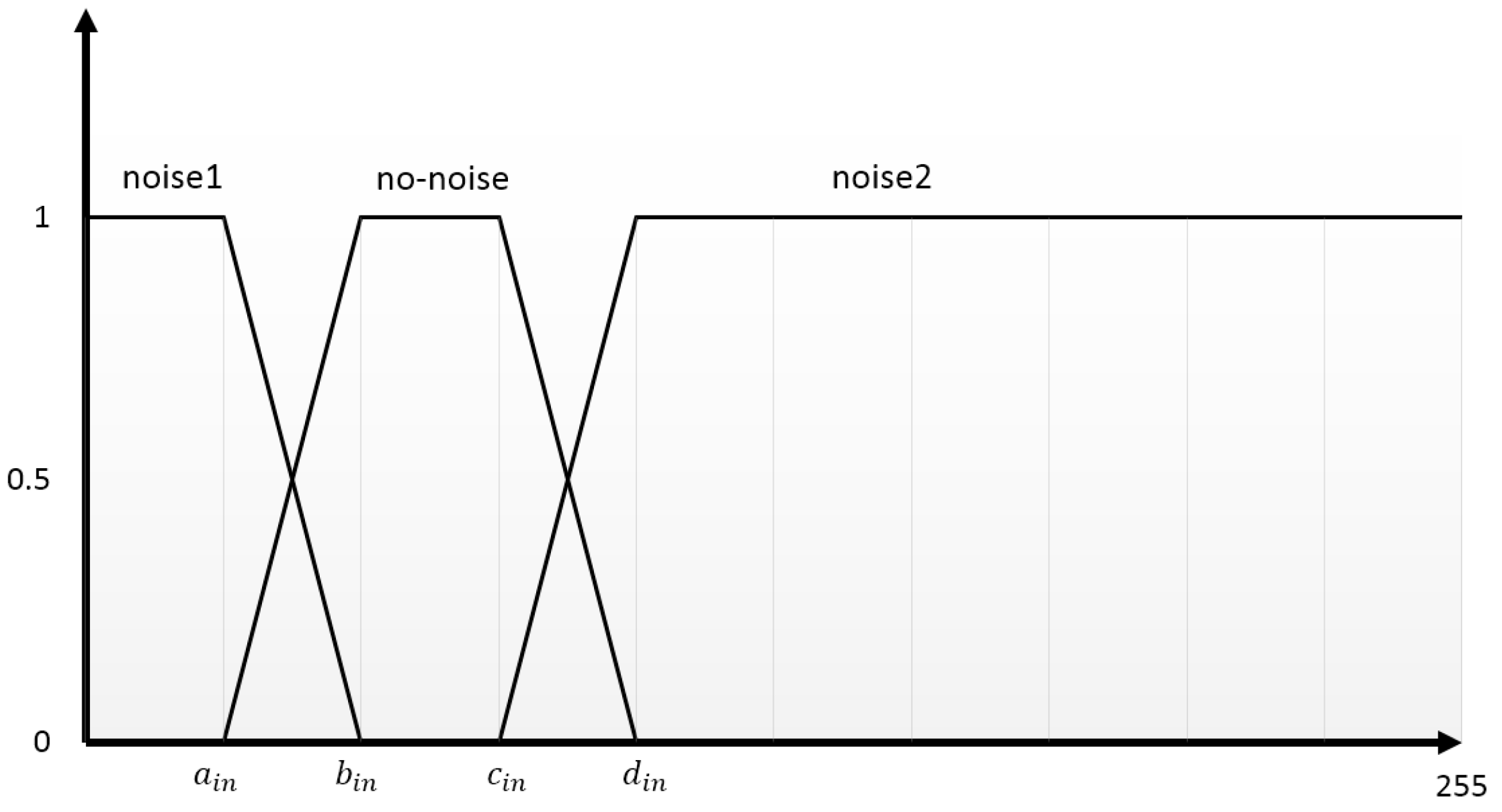
This study uses a method to determine filter order called Sparsity Ranking [27]. Its main idea is that it first selects the region to fix where the noisy ratio is lower, then it better handles more noisy ratio regions later. As the lower noisy ratio region has more uncorrupted pixels, it is easier to restore. Then, there are more useful pixels in the low ratio area for handling noise in more noisy regions.

2.4. Noise Model

When the image is polluted, part of the image will be replaced by impulse noise of a random value. The probability of this noise determines the degree of image deterioration. The noise model is given in Equation (3) below.
x i , j = { o i , j n i , j   w i t h   p r o b a b i l i t y     1 p w i t h   p r o b a b i l i t y     p ,
where p is the noise ratio or probability of noise. x i , j is the pixel value at i row and j column. n i , j and o i , j are pixel intensities of gray-scale images at position ( i , j ) ; they correspond to the original pixel and the noisy pixel, respectively. The pixel intensity of n i , j is between maximum and minimum ( [ I m i n ,   I m a x ] in an 8-bit gray-scale image,   I m i n = 0 ,   I m a x = 255 ). As a result, there are two forms of noise. One form of noise is known as salt and pepper noise. It has a fixed value at both ends of the gray scale. The other type is uniform impulse noise, which has a uniform distribution at [ I m i n ,   I m a x ] and is also known as random-valued impulse noise. The second sort of noise was examined in this research.

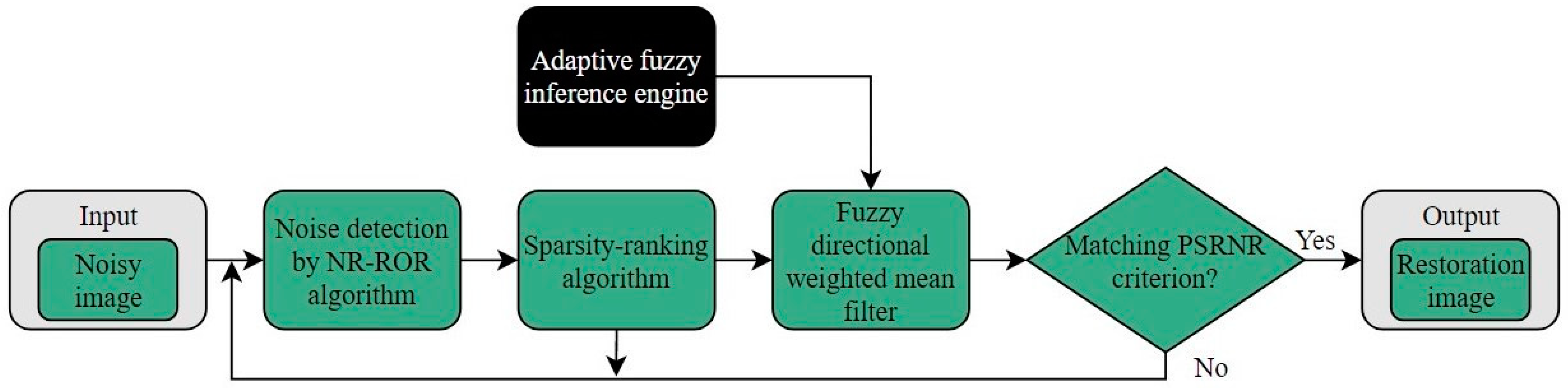
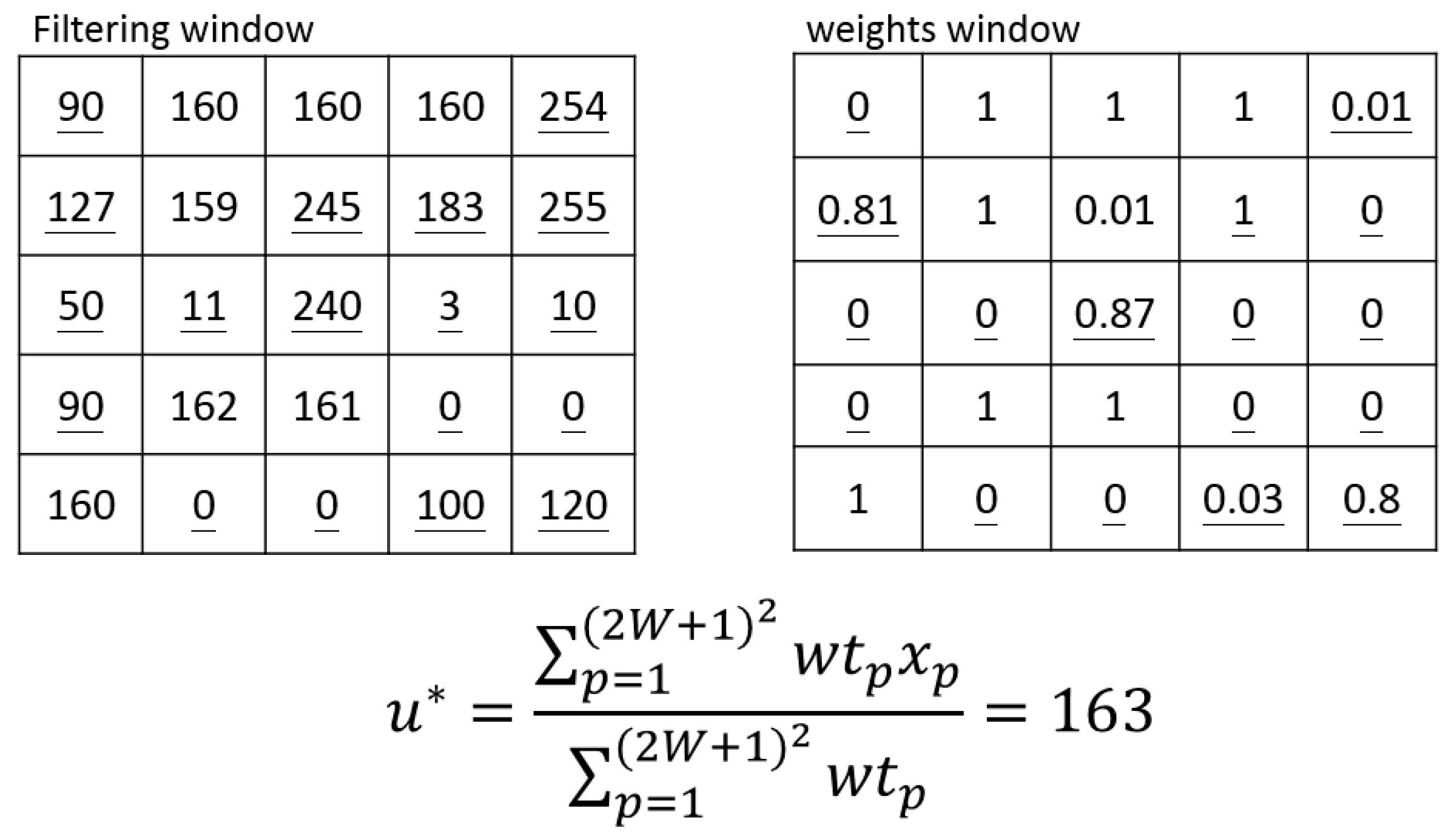
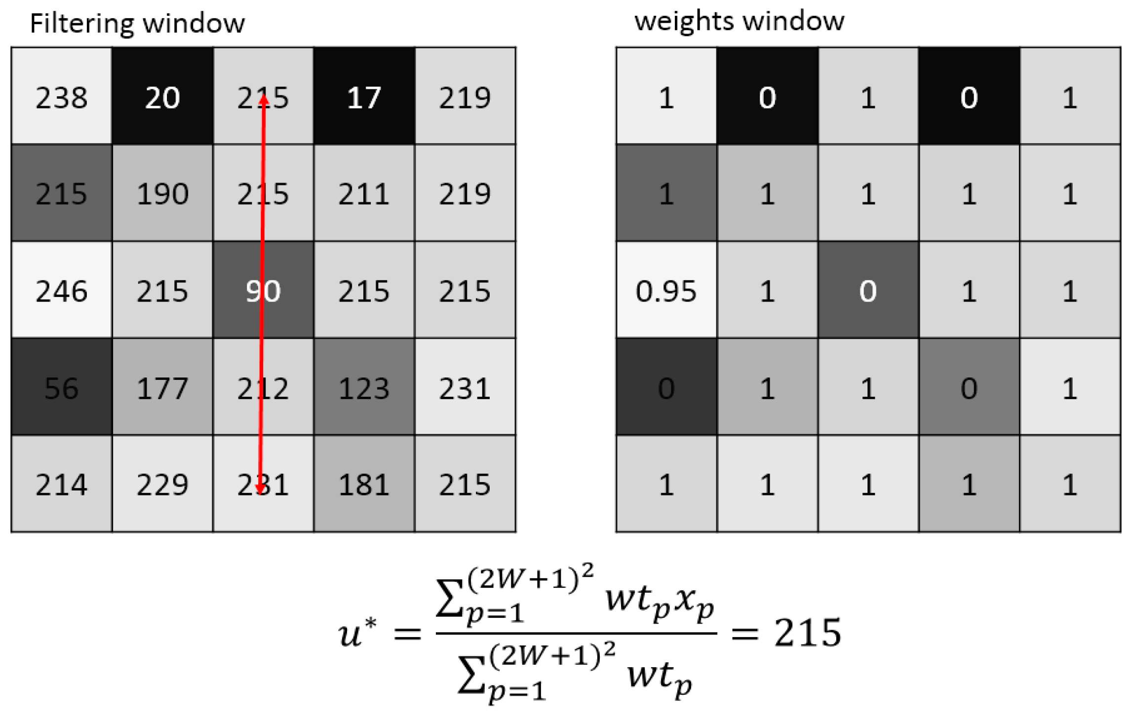
3. The Proposed Adaptive Fuzzy Weighted Mean Filter Model

The proposed AFWMF model can be divided into three stages. The first stage is the proposed detection method, which combines ROR and fuzzy rules to build a corresponding tag matrix. In the second stage, we use a filter order method called sparsity ranking [27]; its main idea and process have been discussed in the previous section. The last stage uses fuzzy rules to filter corrupted pixels according to a tag matrix from the first part, while the filtering order is from the second part. Figure 2 represents the system flowchart of the proposed model, and its key concepts and algorithm of main components are described in the next three subsections.

3.1. Fuzzy ROR Noise Detection

First, the stop iteration condition in the original ROR algorithm is defined as Equation (4).
P S N R c u r P S N R p r e 0.01 ,
where the P S N R c u r represents the peak signal to noise ratio (PSNR) of the current iterative process, and P S N R p r e represents the PSNR of the previous iterative process.
These two PSNRs are compared with the original image; however, the process of restoration does not recognize the original image or the noisy image. Therefore, this study modifies PSNR for stopping iteration. This new stopping condition is called the peak signal-to-removal noise ratio (PSRNR); it can be calculated using fixed images of the previous iteration and the current iteration. PSRNR is defined by extensive experiments and shown as Equations (5) and (6):
P S R N R c u r P S R N R p r e   o r   P S R N R c u r   i s   i n f i n i t e ,
P S R N R = 10 log 10 255 2 1 R C i = 1 R j = 1 C ( x i , j n 1 x i , j n ) 2 ,
where n is the iteration number, x i , j n 1 is the image restoration pixel value in the previous iteration, x i , j n is the image restoration pixel value of the current iteration, P S R N R c u r is the current P S R N R , and P S R N R p r e is the previous P S R N R . By the above P S R N R criteria, the noise detection skill is named the No-Reference ROR (NR-ROR) algorithm in this study.

3.2. Noise Cancellation by Adaptive Fuzzy Directional Weighted Mean

The algorithm we propose is akin to a switching median filter. This filter computes the local image from each picture pixel, rather than only utilizing the median to replace the noise, which is the main difference between our proposed novel method and this filter. More precisely, it utilizes standard deviation and fuzzy inference to estimate the restoration pixel value of the filtering window, where the output of fuzzy inference represents the importance of a pixel. For the above reasons, this filter method is called the AFWMF model in this study. The filtering started after the filtering order was determined as follows: let ρ i , j ( k ) ( k = 1   t o   4 ,   w = 2 ) be a set of four filtering windows directing pixels at one place (i,j). This is defined as follows:
ρ i , j ( 1 ) = { x i 2 , j 2 , x i 1 , j 1 , x i , j , x i + 1 , j + 1 , x i + 2 , j + 2 } , ρ i , j ( 2 ) = { x i , j 2 , x i , j 1 , x i , j , x i , j + 1 , x i , j + 2 } , ρ i , j ( 3 ) = { x i + 2 , j 2 , x i + 1 , j 1 , x i , j , x i 1 , j + 1 , x i 2 , j + 2 } , ρ i , j ( 4 ) = { x i 2 , j , x i 1 , j , x i , j , x i + 1 , j , x i + 2 , j } .
Accordingly, the standard deviation of four filtering window directions is calculated as shown in Figure 3, and the standard deviation measures the degree of data dispersion [28].
σ i , j k = o = 1 N ( ρ i , j ( o , k ) ρ i , j ( k ) ¯ ) 2 N 1   ,   k = 1   to   4 ,
where ρ i , j ( k ) ¯ is the mean value of ρ i , j ( k ) and N represents total number of elements in ρ i , j ( k ) .
Next, minimum standard deviation is formatted and given as follows:
S i , j = m i n {   σ i , j k :   k = 1   t o   4   } ,
where S i , j means that one of the four directions is closest to each other in the same direction. Therefore, the central pixel value of the window should also be close to them in order to preserve the image detail or texture.
For preserving detail or texture, we obtain a reference median from S i , j called R e f M i , j . It is formatted as Equation (10) below.
R e f M i , j = m e d i a n {   S i , j   } .
The standard deviation σ i , j of local windows is defined using Equation (11) below.
σ i , j =   ( X i , j X i , j ¯ ) 2 M 1 , M = ( 2 W + 1 ) × ( 2 W + 1 ) ,
where X i , j ¯ is the mean value of X i , j .
Afterwards, we form membership functions. There are three membership functions corresponding to three input fuzzy sets; they are nosie1, no-noise, and noise2, respectively, and are pictured in Figure 4. In Figure 4, the horizontal axis is a pixel value. On the vertical axis, the grade of membership of the element x in the fuzzy set is shown, with values ranging from 0 to 1. These three membership functions are three input fuzzy sets. They are formatted as Equations (12)–(14) below, respectively.
noise 1 ( x ) = {       1 ,     x a i n b i n x b i n a i n ,     a i n x b i n       0 ,     b i n x ,
no nosie ( x ) = {           0 ,                       x a in x a in b in a in ,     a in x b in                             1 ,     b in x c in d in x d in c in ,     c in x d in       0 ,     d in x ,
nosie 2 ( x ) = {     0 ,     x c i n x c i n d i n c i n ,     c i n x d i n       1 ,     x d i n ,
where a i n = R e f M i , j C 2 × σ i , j ,   b i n = R e f M i , j C 1 × σ i , j ,   c i n = R e f M i , j + C 1 × σ i , j ,   d i n = R e f M i , j + C 2 × σ i , j ,   C 1 C 2 . C 1 and C 2 are parameters that are predefined according to our extensive experiments. R e f M i , j is a reference value that can retain the details of the picture. σ i , j represents the grade of dispersion of the filtering window. Pixels of the window farther from R e f M i , j show that the importance of the pixel is lower; conversely, closer pixels indicate a higher importance. Then, there are two membership functions corresponding to two output fuzzy sets: low and high sets; these are displayed in Figure 5.
In Figure 5, the horizontal axis is the importance value, and it ranges from 0 to 1. On the vertical axis, we have the membership function of a fuzzy set denoted by x, and this axis has values from 0 to 1. These two membership functions are output fuzzy sets. They are defined as Equations (15) and (16) below, respectively.
l o w ( x ) = { O b x O b ,       x O b 0 ,                         x O b ,
h i g h ( x ) = { 0 ,     x O a                 x O a 1 O a ,                 x O a .
In this study, this characteristic is combined with fuzzy inference to decide the weight corresponding to the pixel. The output (the weight corresponding to the pixel) of the fuzzy inference of the proposed AFWMF model is based on three rules of filter stage as follows:
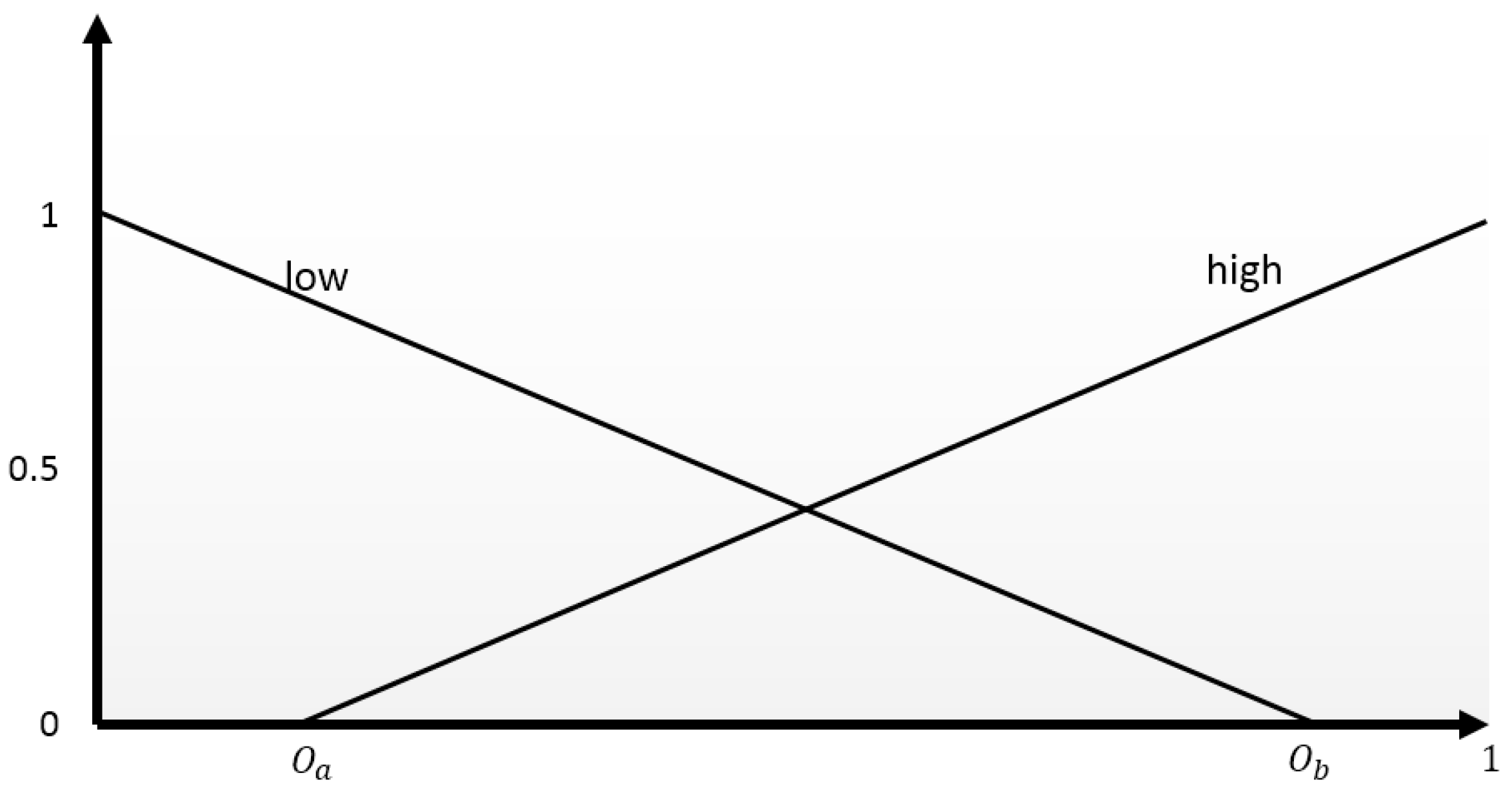
  • Rule 1.IFxi,j is at nosie1, THEN its importance is low.
  • Rule 2.IFxi,j is at noise2, THEN its importance is low.
  • Rule 3.IFxi,j is at no-noise, THEN its importance is high.
Additionally, we can use the above rules to obtain weights. Subsequently, the restoration pixel value u * is calculated and formatted as Equation (17).
u * = p = 1 ( 2 W + 1 ) 2 w t p x p p = 1 ( 2 W + 1 ) 2 w t p ,
where w t p is the weight corresponding to the pixel of filtering window, w t p = 0   t o   1 , w t p W T i , j , W T i , j = { w t s , t | i W s i + W ,   j W t j + W } , x p X i , j . u * is the restoration pixel value, which is regarded as the final output.
In order to preserve details or texture in image and overcome the weakness of median filters, we utilize weights from fuzzy inference. According to Equation (17), the filtering window’s pixel values were multiplied by their associated weights to determine which degree of the pixel should be used to filter in the filtering process. The weight of pixel ω p represents the degree of the R e f M i , j with its immediate surroundings; as a result, it will be utilized to regulate the level of restoration that takes place. Pixel weight ω p indicates the level of importance of the pixel, and this characteristic decides how much useful information is needed for restoring.
Finally, the restoring pixel value is obtained with the weighted mean as the final output and shown as Figure 6, in which the number with an underline means that the pixel is corrupted by noise. Figure 7 shows the noise corruption for a light region. Figure 8 shows the member function according to Equations (10) and (11) for shifting their location. Figure 9 shows the noise corruption for a dark region. Figure 10 is the member function according to Equations (10) and (11) for shifting their location.

3.3. Algorithm of the Proposed AFWMF Model

The algorithm of proposed AFWMF model is summarized in detail below; this is an improved and enhanced version of the ROR algorithm.
  • The enhanced coarse stage includes the following six steps, as follows:
    • Choose parameters for Lc = 1; initialize the flag matrix to all zero.
    • For every pixel in the image, find its ROR, the relative divergence d among the filtering window’s median, and the active pixel.
    • Use the coarse stage of ROR described in Section 2.2 to detect the noise in the active pixel. Good and noisy pixels are represented by zeros and ones, respectively.
    • Following the use of Equations (7)–(14) to build the input membership function and according to three-rules-based filter stage described in Section 3.2, we obtain the pixel weights in a filtering window.
    • By obtaining the value of restoring pixels from Equation (17), let Lc = Lc + 1.
    • Use Equation (5) for judging and stopping the enhanced coarse stage; otherwise, go to Step 2.
  • The enhanced fine stage includes the following six steps:
    • Choose parameters for Lf = 1; initialize the flag matrix to all zeros.
    • For every pixel in the image, find its ROR, the relative divergence d among the filtering window’s median, and the active pixel.
    • Use the fine stage of ROR described in Section 2.2 to detect the noise in the active pixel. Good and noisy pixels are represented by zeros and ones, respectively.
    • Use Equations (7)–(14) to build the input membership function. According to the three rules-based filter stage described in Section 3.2, obtain the pixel weights in the filtering window.
    • By obtaining the value of restoring pixel from Equation (17), let Lf = Lf + 1.
    • Use Equation (5) for judging and stopping the enhanced fine stage; otherwise, go to Step 2.

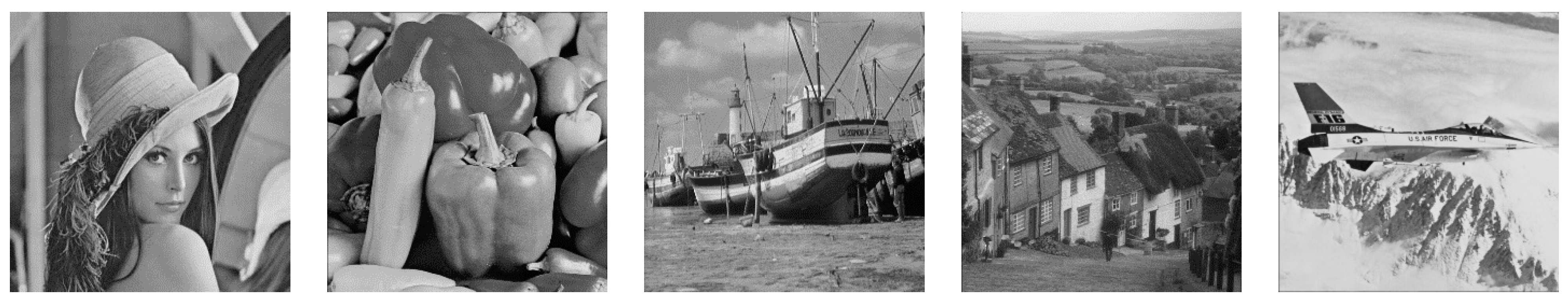
4. Experiment Results and Discussions

Initially, the estimate matrix for filters, including the mean square error (MSE) and the PSNR, is defined and determined using Equations (18) and (19), respectively. The MSE can be used to compute the PSNR, and the PSNR is a quantitative indicator for evaluating the performance of different filters. Importantly, the smaller the value of MSE is, the better the performance is. Conversely, the PSNR is bigger for a better performance. Moreover, this study uses another quantitative indicator, structural similarity index measure (SSIM), for further measuring the filtering performance, and its formula is defined as Equation (20) below. The SSIM value is an index that is mainly used to predict the perceived quality of digital images and measure the similarity between two images. The difference between the PSNR value and the SSIM value is that the former method estimates absolute errors, and the latter has the structural information that the pixels have strong inter-dependencies when they are spatially close to each other. More importantly, both the PSNR and SSIM values are effective evaluation standards from past studies.
M S E = 1 R × C i = 1 R j = 1 C ( O i , j Y i , j ) 2 ,
P S N R = 10 l o g 10 ( 255 2 M S E ) ,
S S I M = ( 2 μ O μ Y + e 1 ) ( 2 σ O Y + e 2 ) ( μ O 2 + μ Y 2 + e 1 ) ( σ O 2 σ Y 2 + e 2 ) ,
where R and C represent the dimensions of the image and R × C is the size of an image. O represents the original image and Y is the image that has been restored. The SSIM gives the similarity measurement between the original and restored image as in Equation (20), where μ O and μ Y are the mean intensities of the original and restored images, σ O and σ Y are the standard deviations of the original and restored images, σ O Y is the covariance of the original image and restored image, e 1 = ( k 1 L ) 2 , e 2 = ( k 2 L ) 2 , L is the dynamic range of the pixel values, and k 1 and k 2 are regularization parameters.
To further verify the performance of the proposed AFWMF model, five famous testing pictures, including Lena, Peppers, Boat, Gold Hill, and Plane, respectively, are used in this study for the image-processing experiments. They are pictured in Figure 11, which was generated by an 8-bit grey level. All their resolutions are 512 by 512. In order to make the experiments more general and precise, this study conducted two experiment evaluations. One compared the PSRNR of the AFWMF model with the PSNRs of different filters; the other compared the psycho-visual result of the AFWMF model with the psycho-visual results of different filters. The different filters are addressed in BDND [9], DWM [16], EAIF [22], FRDFM [18], SBF [3], SDOOD [29], ROR [25], ASMF [12], and EBDND [30], since they were all identified to have good performances in the literature reviews in this area. The experimental results are described with measurement indexes in the next four subsections, and these results and the different filters are discussed in the last subsection.

4.1. Restoration Performance Measurements

This evaluation standard of the performance test uses Equation (19), and the Lena image is first used to compare the proposed AFWMF model with other filters proposed by other studies. The characteristic Lena image has an approximately normal distribution; that is to say that the detail, flat regions, shading, and texture are all included. Thus, the Lena image is an excellent comprehensive testing image for assessing restoration results and comparing restoration performance. Table 3 shows the comparison of the PSNR measurement values in the Lena image; the noise is set from 10% (i.e., 0.1) to 90% (i.e., 0.9). (Note: to lower the overabundance of figures and tables, this study only uses the empirical results of the Lena image as a representative of the demonstration here, but it uses a summary report of a table for completely concluding the results of the five images in this subsection.) From Table 3, it can be seen that the AFWMF model has a slightly worse PSNR value than that of the DWM and ROR filters in the low 10% noise density instance and high 80–90% noise density instance. However, the AFWMF model’s PSNR value apparently outperforms the other filter techniques at higher ratios of 20% to 70% noise densities. Importantly, when the ratio of noise density is within 20–70%, the proposed AFWMF model significantly outperforms all the existing filters selected and used for the Lena image in this study. For processing the Lena image, it is ranked in the order AFWMF > DWM > ROR > ASMF > SDOOD > SBF > FRDFM > EAIF > BDND > EBDND in PSNR performance. The proposed AFWMF model is the best filtering model used for the Lena image.
For further evaluating the performance of all the five images used in this study, Table 4 and Figure 12 show the additional comparisons of the PSNR average measurements for noise of 10% to 90%. From the above table and figure, this is ranked in the same order as the Lena image of AFWMF → DWM → ROR → ASMF → SDOOD → SBF → FRDFM → EAIF → BDND → EBDND in terms of the performance of the PSNR average value for the five images. Thus, this is effective evidence that the proposed AFWMF model has the best filter technique in this study. Furthermore, Table 5 presents the best filter model at different noise densities in the PSNR average value for the five experimental images. It is found that it is best to use the DWM model for a low 10% noise density, the ROR model for high 80% to 90% noise densities, and the AFWMF model for 20% to 70% noise densities.

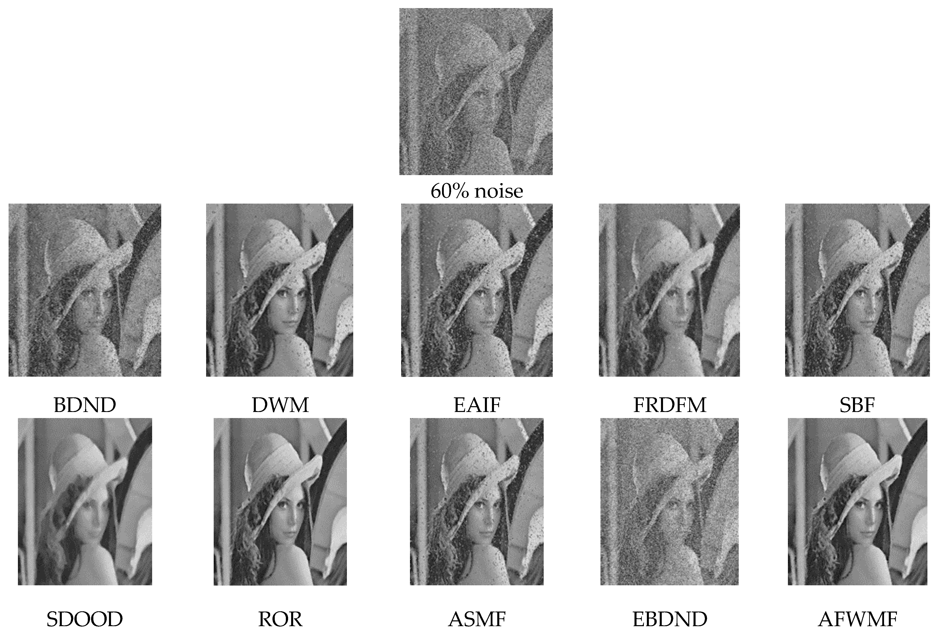
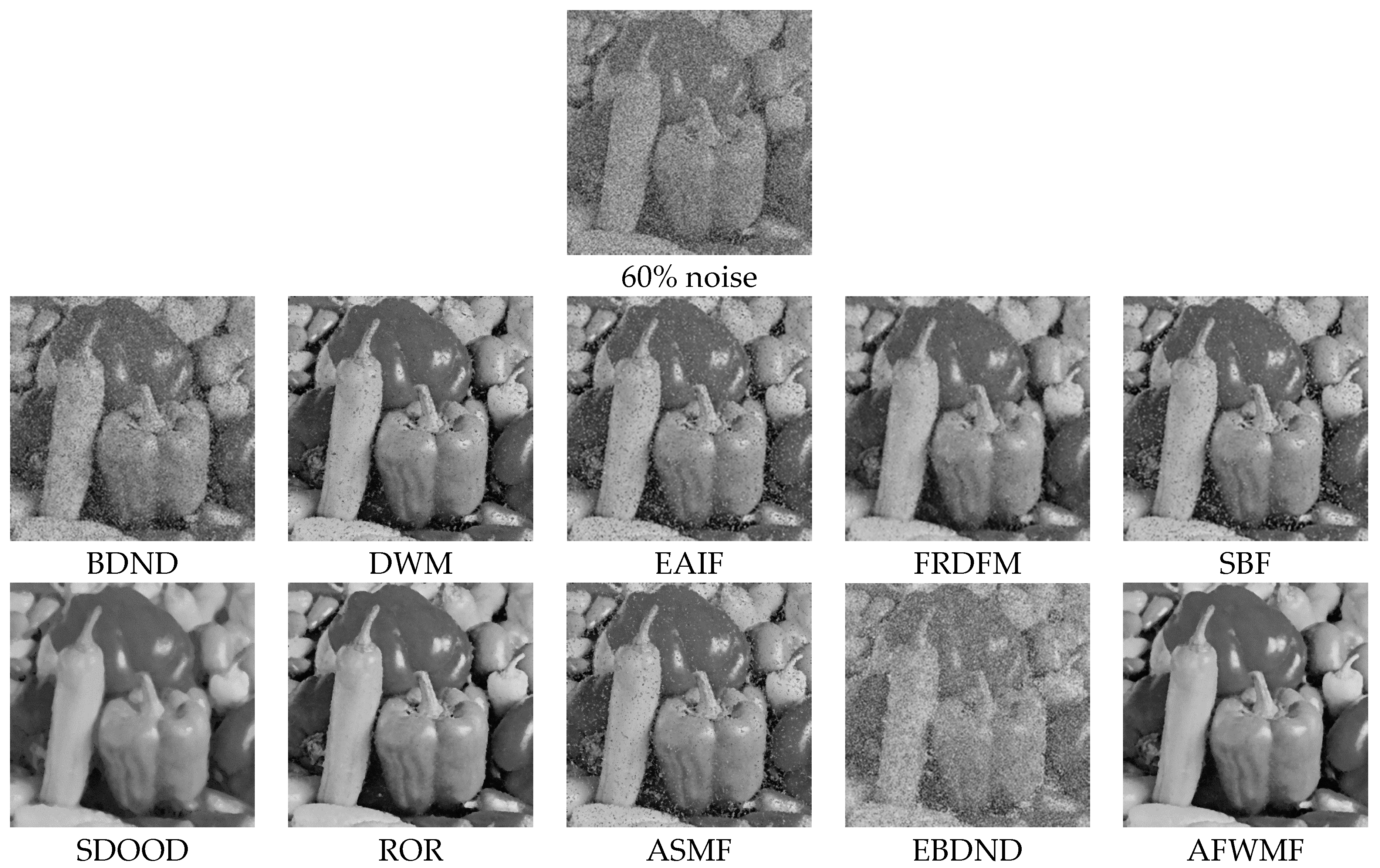
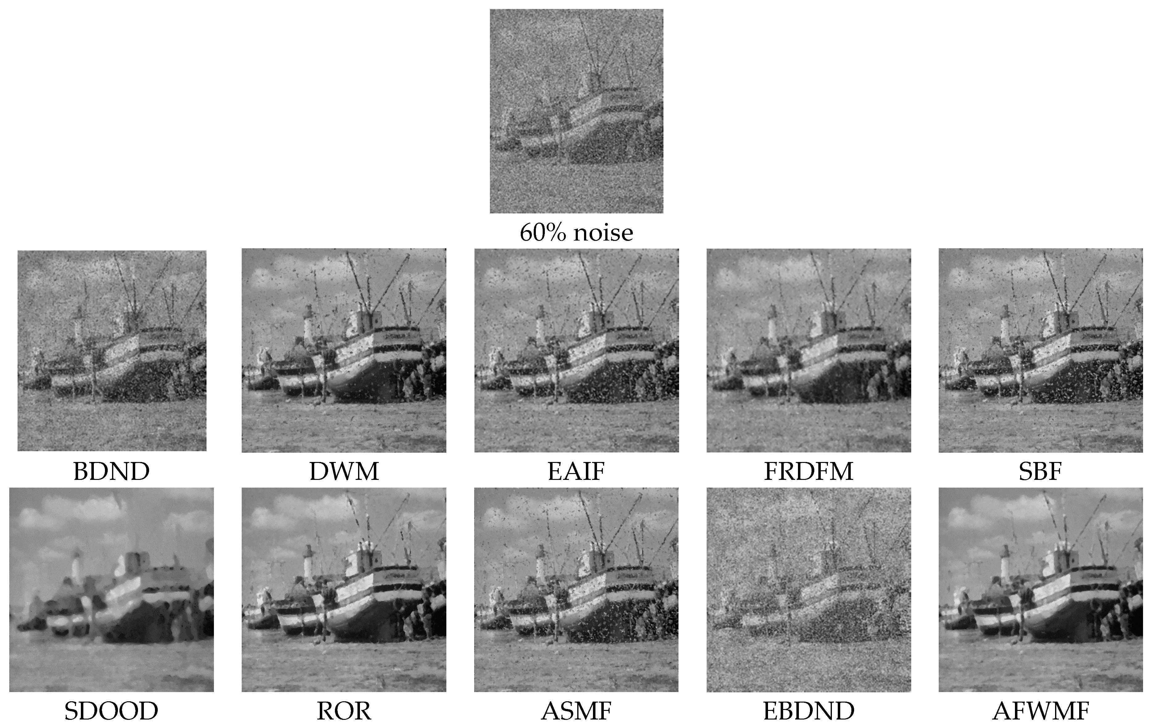
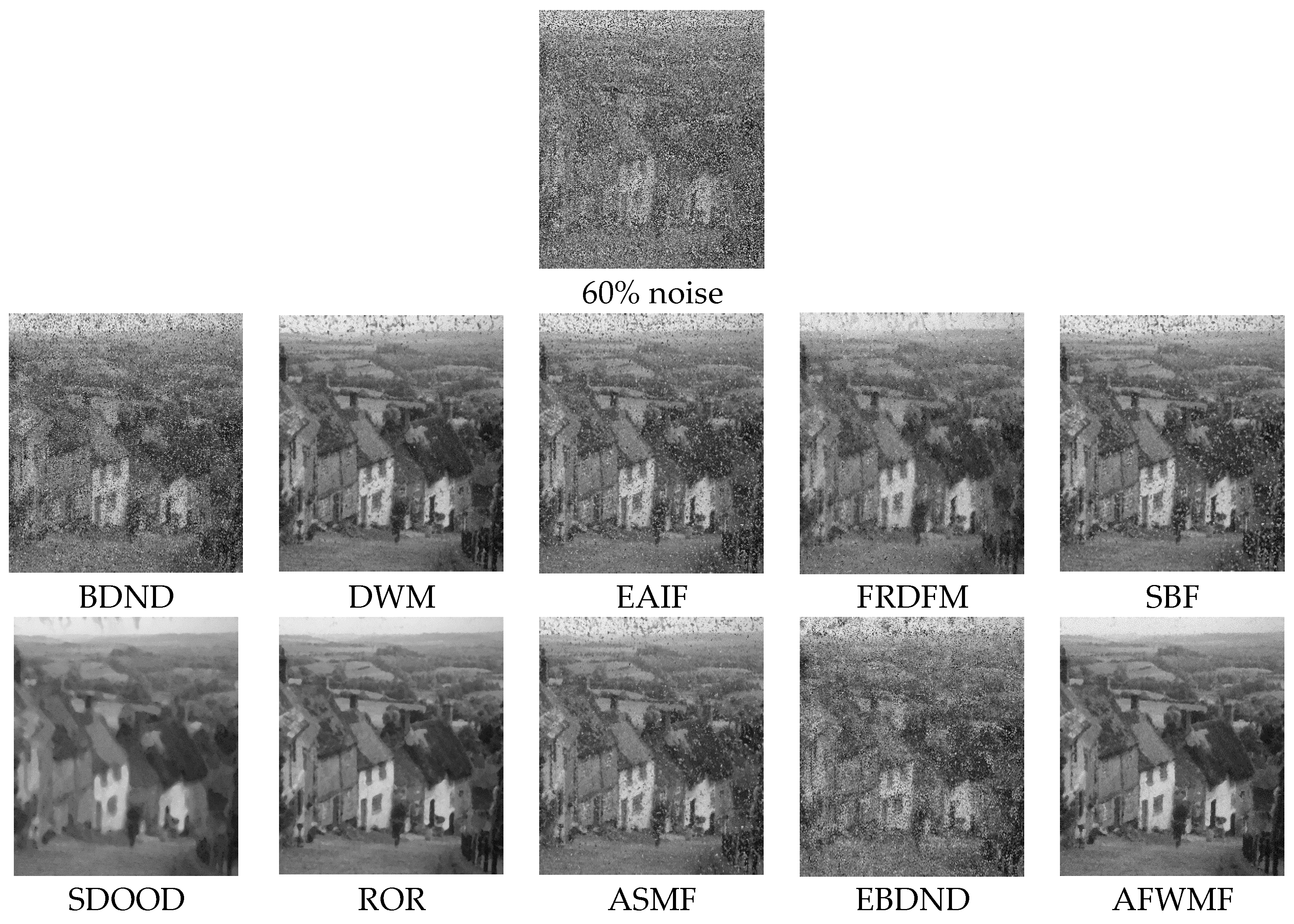
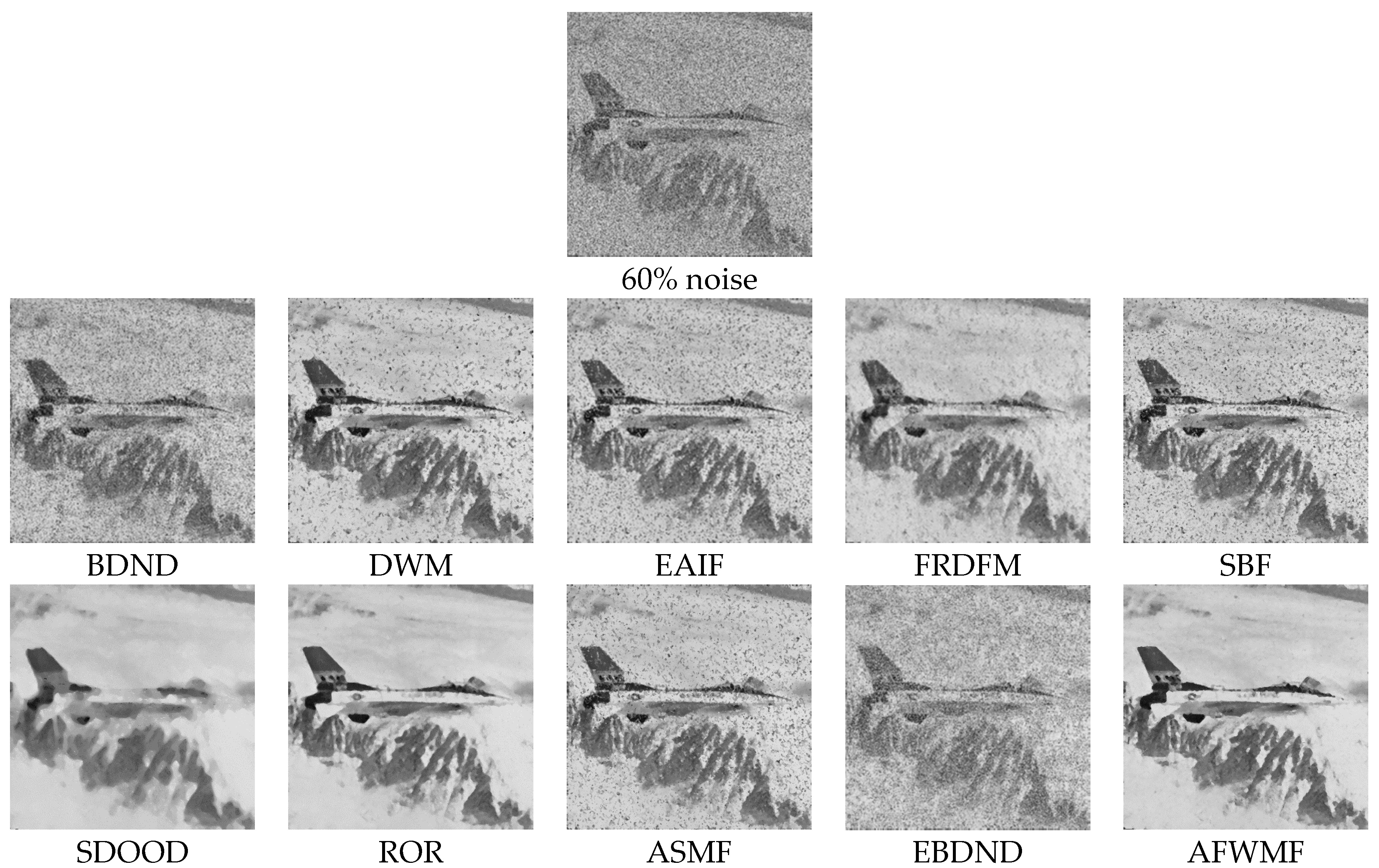
4.2. Psycho-Visual Performance Comparison

In order to evaluate the psycho-visual performance in detail preservation, this experiment uses the real restoration image as the testing target to measure different filters for all the five images used. The noise is also set in ratios of 10–90% noise densities, but the 60% random-valued impulse noise here is selected randomly and contaminated in the first figure for the result presentation of the psycho-visual test in this study. Thus, the experiments are run for evaluating the restoration images at 60% noise density (note: due to the need to cut down the complexity of excessive figures and tables, this study only displays the empirical results of 60% noise densities as a representative figure presentation for the five images in this subsection). As a result, Figure 13, Figure 14, Figure 15, Figure 16 and Figure 17 show the measurement results for the psycho-visual performance comparison in these images for assessing different filtering techniques. Obviously, the proposed AFWMF model is still preferable when compared to the other filtering models by personal observation; however, in order to identify the testing results of psycho-visual comparison, this study invited three experts who specialize in this image processing field to help with the visual evaluation. In particular, Table 6 shows the average ranking of the performance comparison for a noise of 60% made by the three experts. In Table 6, it is indicated that the proposed AFWMF model is still the best one and has a better performance in psycho-visual testing for a ratio of 60% impulse noise density. From Table 6 and these figures, it is clear that the top three models are AFWMF, ROR, and DWM in terms of rank ordering. It is shown that the proposed AFWMF model has better performance than other filtering models in terms of psycho-visual comparison and recognition for various testing points, such as shading, flat regions, detail, and edge, from the experts.
In addition, to further evaluate the key impact of the 10 filtering models used for noise interference processing, this study also further describes different levels of noise density for the image processing to improve the visual evaluation of the three experts. They again ranked the images restored by the 10 filters from 10% to 90% of interference for the five experimental images. Subsequently, the average ranking of the performance by the same three experts was calculated and is shown in Table 7, Table 8 and Table 9 for different levels of noise: 30% (low), 50% (median), and 70% (high), respectively. From Table 7, Table 8 and Table 9, it is also clear that the proposed AFWMF model performs the second best at a 30% noise density and is the best one in both the 50% and 70% noise densities. In general, the proposed AFWMF model still has the best performance in psycho-visual comparison for the five images compared to the other listed filtering models both generally and comprehensively. Productively and meaningfully, the proposed AFWMF model has a better performance than the other listed filtering models in terms of psycho-visual comparison, regardless of the level (low, medium, or high) of noise density involved. Thus, extra experiments are further needed to provide this evidence in other ways or in other images.

4.3. Stop Iteration Comparison

It is important to understand the iterative condition of the related ROR algorithm under the picture (or image) and its noise density. In this experiment, this study can interestingly verify the new stop criteria to stop iteration under the original image and noise density unknown and avoid the picture being over-repaired (i.e., the detail texture is removed). Regarding the environment of iteration, the stop condition is set up under the same ROR iterative architecture and the median filter is used to filter out the noise. The iteration number of the original ROR is shown in Table 2, which is based on the original image and the noise density. Referring to Equations (4)–(6), (18) and (19), the number of iterations for the new conditions is provided in this study. Furthermore, the noise density is selected at the low, medium, and high noise levels (30%, 50%, and 70%, respectively) from Table 2 using the same five images.
As a result, the average PSNR of the five images for the verification results is shown in Table 10 and Table 11, referring to Table 2 and using Equations (5) and (6), respectively. Table 10 uses the number of iterations estimated from the original ROR, while the stop condition using the PSRNR formula is obtained under the principle of an unknown original image and no noise information in Table 11. In the tables, it is shown that the comparable results of the PSNR value for the proposed AFWMF model are very close to the original ROR method, which uses the known noise density conditions. Therefore, the experimental results show that the proposed AFWMF model can effectively support the stop criterion for the iteration and obtain a set of optimal PSNR values that is very close to the known information conditions of the original image.
Afterwards, it is also necessary to compare the PSRNR algorithm with the original ROR algorithm in different parameters to its noise density in Table 2. In fact, the noise density and the original image are not known when the noise is filtered out, and it is not possible for the iteration number to refer to Table 2 from the original ROR method. Therefore, for the experimental fairness of the testing results, the implementing process was tested under the same ROR architecture and the same noise density as that in Table 2. That is, the noise density is also selected in the same low, medium, and high noise levels (30%, 50%, and 70%) for performance comparison. The experimental results are shown in Table 12, Table 13, Table 14, Table 15 and Table 16 for the five images. It is found that in most cases (about 10/15 = 0.67), the empirical result can be very close to the repair effect found in Table 2, where the proposed PSRNR method is used as the stop condition. Thus, the proposed AFWMF model still conclusively has the best result out of all the filter techniques used in this study.

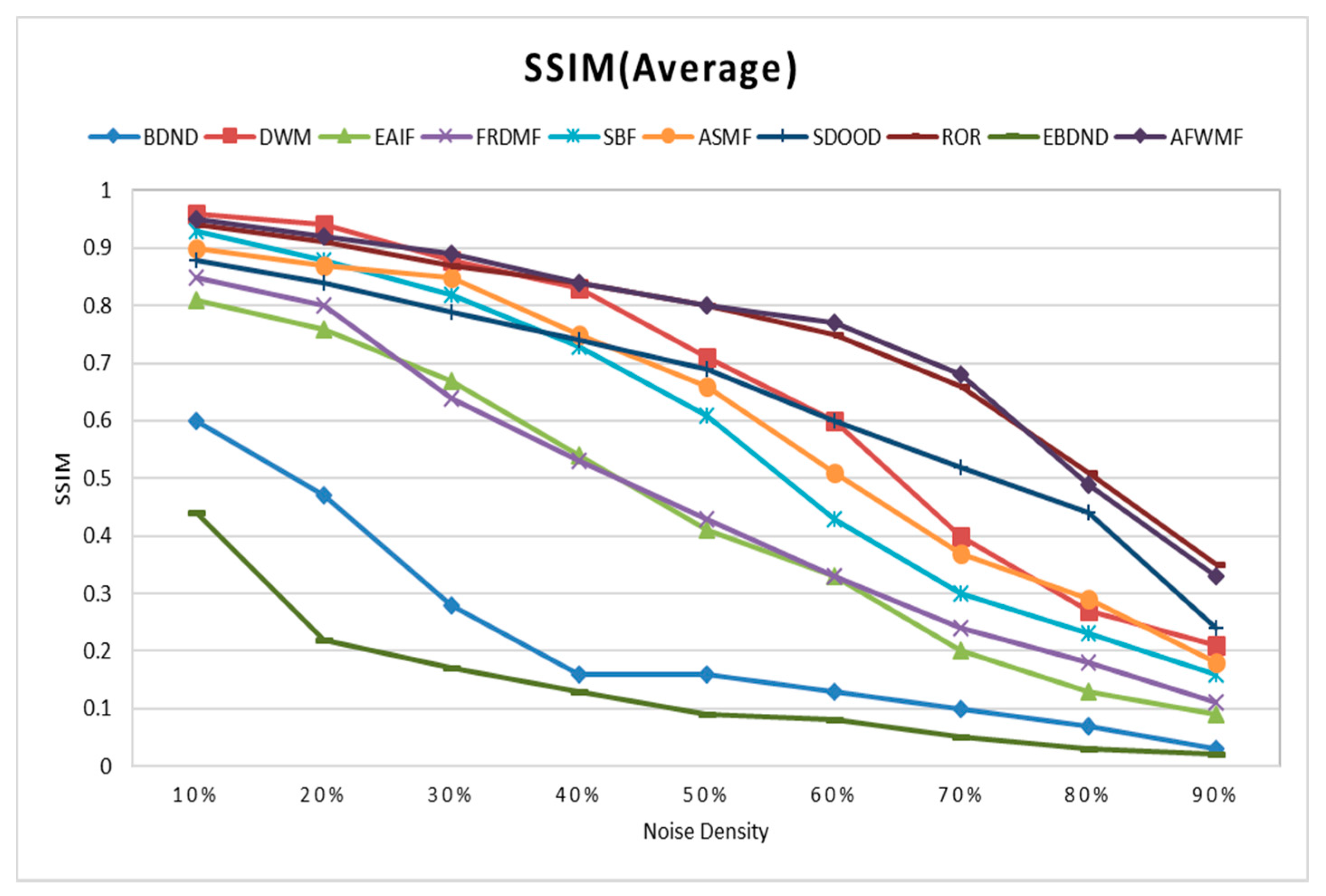
4.4. Performance Comparison of SSIM

Afterwards, to further deeply reidentify the performance of the 10 filtering models, this study uses the second measurement indicator (i.e., SSIM value) for processing the noise density of images. Thus, Table 17 and Figure 18 show the SSIM average value at different noise densities from the 10 filter models for the five experimental images. Regarding the empirical results, it is found that the ranking order is AFWMF → ASMF → DWM → ROR → SDOOD → SBF → FRDFM → EAIF → BDND → EBDND in terms of the performance of the SSIM average value. From Table 4 and Table 17, two interesting and meaningful findings are defined and determined. (1) The proposed AFWMF model is the best one for processing impulse noise density regardless of the PSNR and SSIM values. (2) It is also important to find an appropriate filtering method for use in a variety of images.

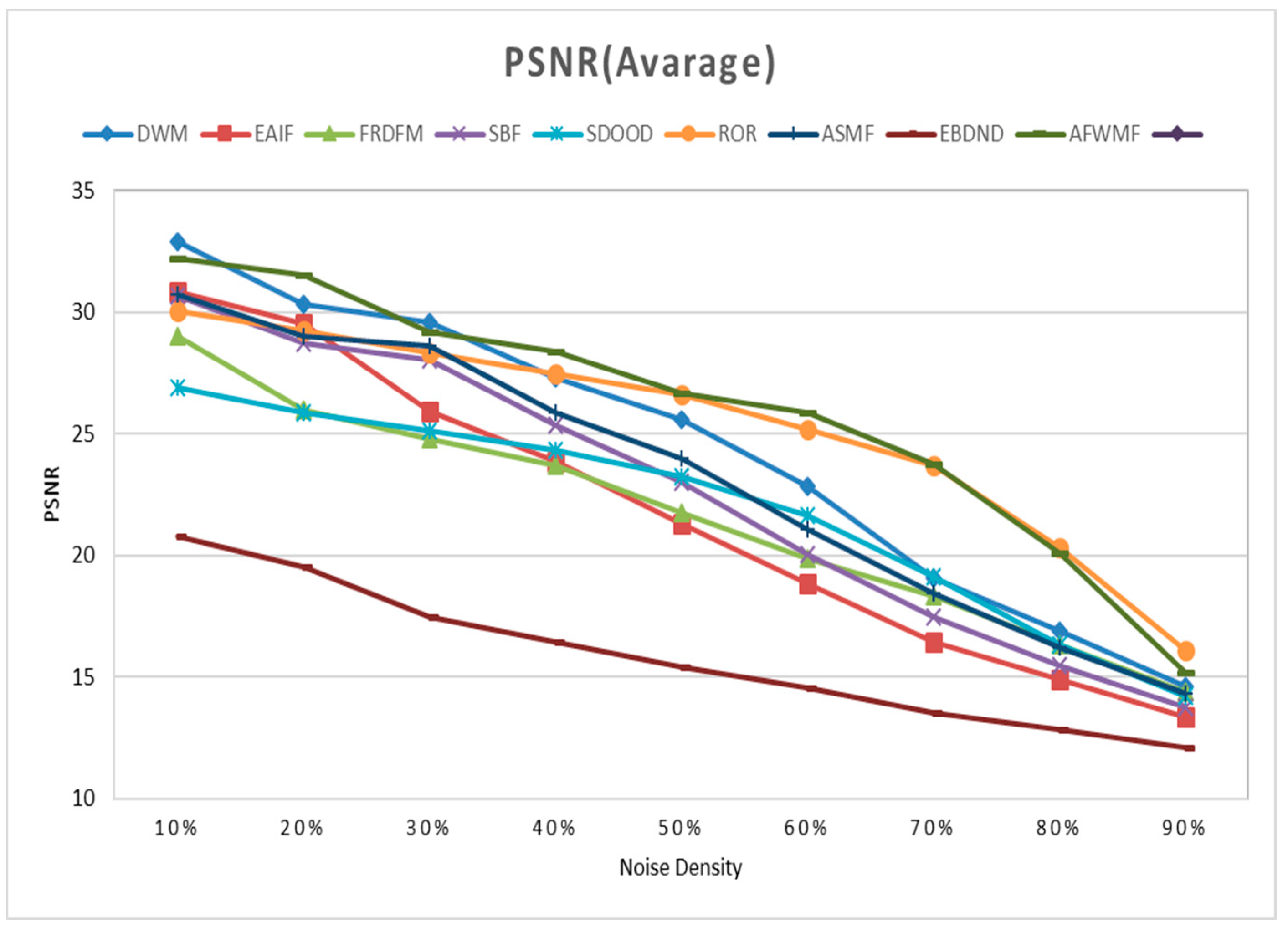
4.5. Discussions for the Related Results

From all the experimental results, the study raises some questions related to the different filtering models in the following two directions: (1) The AFWMF model is the best method for denoising signals in almost all noise levels to the Lena, Gold Hill, and Boat images; however, the performance in the Peppers and Plane images is slightly worse in terms of some ratios of noise density when compared to the DWM and ROR models. The possible reasons for the issues mentioned above are that the AFWMF model improves its filtering performance using a more complicated and varied feature, form, or style than that of the other listed filtering models mentioned in this study. (2) The relationship between PSNR and noise density in the 10 listed filter models and the advantages/disadvantages or characteristics of the 10 filter models are discussed in the following: (a) The BDND filter is proven to operate efficiently even under high noise densities. However, the critical parameter needs to be defined in the filtering step of the BDND algorithm. (b) The DWM is based on the differences between the current local pixel and its neighbors aligned with four main directions. Then, the minimum of these four direction indexes is used for impulse detection. It makes full use of the characteristics of impulse and edges to detect and restore noise. DWM has an excellent performance in low-noise conditions. (c) The EIAF algorithm consists of two steps: impulse noise fuzzy detection and impulse noise cancellation. The EAIF has a slightly better performance in PSNR evaluation with 10% and 20% noise. It ranks eighth out of ten models. (d) FRDFM generally has a better performance at a higher noise percentage. For example, under 80% and 90% noise, it ranks fifth among the 10 model methods. However, it only ranks seventh in terms of its overall ranking. (e) SBF ranks sixth overall and has an average performance at various noise percentages. (f) SDOOD ranks fifth, but he ranks poorly in low noise and better in high noise conditions, ranking third with 90% noise. (g) The ROR method does not necessarily have a good performance in the state of low noise, because ROR is an improvement mechanism for DWM under high noise, so it has a better performance under high noise. It is in third place. (h) The method of using ASMF has a good performance under various noise conditions. Its overall ranking is fourth. (i) The EBDND is used for some special cases, so it is more difficult to define the critical parameters. Thus, it does not have a good performance without the definition of special parameters. It has the worst performance in terms of PSNR evaluation. (j) The proposed AFWMF method uses the combined benefits of ROR, DWM, and others, so its overall average has the best performance.

5. Conclusions

This study has proposed a new filtering framework called the AFWMF model. We proposed four key points and concerns relating to the image processing abilities of this new model. (1) First, this study transforms the original ROR algorithm to an expert system of fuzzy inference, since the use of fuzzy sets of fuzzy inference is a multi-value concept. Thus, the original ROR algorithm is combined with fuzzy inference in the proposed model; then, the empirical results show that the fuzzy ROR can be used more precisely to find noise from pictures (images). (2) Second, this study proposes a new stop condition of PSRNR. In the literature [12,16,25], the noise density and original image are used as references or standards for stop iteration; however, these studies exhibit some drawbacks (or problem), as they do not know what the original image or noise density is. Interestingly, the proposed PSRNR can bridge the gap of the above problem. (3) Third, in general, the median filter only uses a majority decision strategy. This strategy has a serious problem: the median filter is ineffective in filtering out noise when the noise density is over 50%. Thus, this study combines the use of directional medians and fuzzy inference to overcome this problem. (4) Finally, this study uses the fuzzy inference membership function, which can shift dynamically to accommodate random-valued impulse noise according to the distribution of the filter window; thus, it can improve the performance of image processing.
The five well-known images, Lena, Peppers, Boat, Gold Hill, and Plane, were used as the experimental targets for evaluating the proposed AFWMF model. After all the experiments were run, this novel AFWMF model was found to significantly improve processing performances in the measurement of the PSNR value for preserving detail and fixed images at noise densities within the range of 20% to 70% for the experimental images. In extensive experiments, the method described in this study also showed a better performance in evaluating psycho-visual tests and identifying PSRNR than the other listed filter methods. Furthermore, the proposed AFWMF model also has better indicator of SSIM value. Conclusively, the proposed AFWMF model was generally found to be the best model among the listed 10 filtering methods for image processing in terms of the measurement of two quantitative indicators: PSNR and SSIM. From the experiments, five directions were found for presenting the empirical results of the proposed AFWMF model. (1) The proposed AFWMF model had a better performance in terms of the PSNR value and psycho-visual testing than the other filters for different random-valued impulse noises; however, the random-valued impulse noise is very difficult to remove from the related review of the scarce literature. (2) The proposed AFWMF model performed well in terms of restoration performance and sense of sight in this study. (3) The proposed AFWMF model showed a better restoration of detail or texture than the other filters, especially when the noise density ratio was within the range of 20 to 70%. (4) In total, this study provides good evidence that the proposed AFWMF model performs better in terms of PSNR and SSIE values. (5) Meaningfully, it was found that different impulse noise densities should be used with different filtering methods. It is important to find a suitable filtering model for processing images with various noise densities.
Interestingly, three meaningful findings for subsequent image processing applications were identified: (1) The proposed AFWMF model was the best one for processing different impulse noise densities in terms of both the PSNR and SSIM values. (2) It is important to find an appropriate filtering method for use with a variety of images. (3) From the empirical results, it is evident that the DWM model can be used for a low 10% noise density, the ROR model can be used for high 80% and 90% noise densities, and the AFWMF model can be used with 20–70% noise densities. Although the study shows some benefits of image processing, our techniques still need to be improved. For example, providing a new resolution for image processing will be necessary in future research.

Author Contributions

Conceptualization, J.-R.C. and H.-C.C.; methodology, J.-R.C.; software, H.-C.C.; validation, J.-R.C., Y.-S.C. and C.-M.L.; formal analysis, J.-R.C.; investigation, J.-R.C.; resources, H.-C.C.; data curation, H.-C.C.; writing—original draft preparation, J.-R.C.; writing—review and editing, Y.-S.C. and C.-M.L.; visualization, Y.-S.C.; supervision, C.-M.L.; funding acquisition, C.-M.L. All authors have read and agreed to the published version of the manuscript.

Funding

This research received no external funding.

Institutional Review Board Statement

Not applicable.

Informed Consent Statement

Not applicable.

Data Availability Statement

Publicly available datasets were analyzed in this study. The data can be found here: [https://links.uwaterloo.ca/Repository.html] accessed on 26 July 2021.

Conflicts of Interest

The authors declare no conflict of interest.

References

  1. Bull, D.R.; Zhang, F. Intelligent Image and Video Compression, 2nd ed.; Academic Press: London, UK, 2021. [Google Scholar] [CrossRef]
  2. Kok, C.-W.; Tam, W.-S. Image Quality. Digital Image Interpolation in Matlab; Wiley-IEEE Press: New York, NY, USA, 2019; pp. 71–89. [Google Scholar] [CrossRef]
  3. Lin, C.-H.; Tsai, J.-S.; Chiu, C.-T. Switching bilateral filter with a texture/noise detector for universal noise removal. IEEE Trans. Image Process. 2010, 19, 2307–2320. [Google Scholar] [PubMed]
  4. Vasanth, K.; Varatharajan, R. An adaptive content based closer proximity pixel replacement algorithm for high density salt and pepper noise removal in images. J. Ambient Intell. Hum. Comput. 2020. [Google Scholar] [CrossRef]
  5. Zheng, Y.; Zhao, Y.; Zhou, N.; Wang, H.; Jiang, D. A short review of some analog-to-digital converters resolution enhancement methods. Measurement 2021, 180, 109554. [Google Scholar] [CrossRef]
  6. Vasanth, K.; Varatharajan, R. A decision based unsymmetrical trimmed modified winsorized variants for the removal of high-density salt and pepper noise in images and videos. Comput. Commun. 2020, 154, 433–441. [Google Scholar]
  7. Thanh, D.N.; Hien, N.N.; Kalavathi, P.; Prasath, V.S. Adaptive switching weight mean filter for salt and pepper image denoising. Procedia Comput. Sci. 2020, 171, 292–301. [Google Scholar] [CrossRef]
  8. Sadrizadeh, S.; Zarmehi, N.; Kangarshahi, E.A.; Abin, H.; Marvasti, F. A fast iterative method for removing impulsive noise from sparse signals. IEEE Trans. Circuits Syst. Video Technol. 2021, 31, 38–48. [Google Scholar] [CrossRef] [Green Version]
  9. Ng, P.-E.; Ma, K.-K. A switching median filter with boundary discriminative noise detection for extremely corrupted images. IEEE Trans. Image Process. 2006, 15, 1506–1516. [Google Scholar]
  10. Shah, A.; Bangash, J.I.; Khan, A.W.; Ahmed, I.; Khan, A.; Khan, A.; Khan, A. Comparative analysis of median filter and its variants for removal of impulse noise from gray scale images. J. King Saud Univ. Comput. Inf. Sci. 2020. [Google Scholar] [CrossRef]
  11. Shu, L.; Du, H. Side window weighted median image filtering. In Proceedings of the 2020 5th International Conference on Multimedia Systems and Signal Processing, Chengdu, China, 28–30 May 2020; Association for Computing Machinery: New York, NY, USA, 2020; pp. 26–30. [Google Scholar] [CrossRef]
  12. Sohi, P.J.S.; Sharma, N.; Garg, B.; Arya, K.V. Noise density range sensitive mean-median filter for impulse noise removal. In Innovations in Computational Intelligence and Computer Vision; Advances in Intelligent Systems and Computing; Sharma, M.K., Dhaka, V.S., Perumal, T., Dey, N., Tavares, J.M.R.S., Eds.; Springer: Singapore, 2020; Volume 1189. [Google Scholar] [CrossRef]
  13. Sheela, C.J.; Suganthi, G. An efficient denoising of impulse noise from MRI using adaptive switching modified decision based unsymmetric trimmed median filter. Biomed. Signal Process. Control 2020, 55, 101657. [Google Scholar] [CrossRef]
  14. Bhargava, P.; Prasad, A. Diminishing impulse noise using fuzzy switching median filter. Int. J. Adv. Res. Sci. Commun. Technol. 2020, 1, 60–65. [Google Scholar]
  15. Tao, C.; Kai-Kuang, M.; Li-Hui, C. Tri-state median filter for image denoising. IEEE Trans. Image Process. 1999, 8, 1834–1838. [Google Scholar]
  16. Singh, I.; Verma, O.P. Impulse noise removal in color image sequences using fuzzy logic. Multimed. Tools Appl. 2021, 80, 18279–18300. [Google Scholar] [CrossRef]
  17. Kang, C.C.; Wang, W.J. Modified switching median filter with one more noise detector for impulse noise removal. Int. J. Electron. Commun. Assoc. Comput. 2008, 63, 998–1004. [Google Scholar] [CrossRef]
  18. Kang, C.C.; Wang, W.J. Fuzzy reasoning-based directional median filter design. Signal Process. 2009, 89, 344–351. [Google Scholar] [CrossRef]
  19. Ibrahim, H.; Pik Kong, N.S.; Ng, T.F. Simple adaptive median filter for the removal of impulse noise from highly corrupted images. IEEE Trans. Consum. Electron. 2008, 54, 1920–1927. [Google Scholar] [CrossRef]
  20. Srinivasan, K.S.; Ebenezer, D. A new fast and efficient decision-based algorithm for removal of high-density impulse noises. IEEE Signal Process Lett. 2007, 14, 189–192. [Google Scholar] [CrossRef]
  21. Liang, S.; Lu, S.; Chang, J.; Lin, C. A novel two-stage impulse noise removal technique based on neural networks and fuzzy decision. IEEE Trans. Fuzzy Syst. 2008, 16, 863–873. [Google Scholar] [CrossRef]
  22. Luo, W. An efficient algorithm for the removal of impulse noise from corrupted images. Int. J. Electron. Commun. 2007, 61, 551–555. [Google Scholar] [CrossRef]
  23. Aizenberg, I.; Butakoff, C.; Paliy, D. Impulsive noise removal using threshold Boolean filtering based on the impulse detecting functions. IEEE Signal Process Lett. 2005, 12, 63–66. [Google Scholar] [CrossRef]
  24. Crnojevic, V.; Senk, V.; Trpovski, Z. Advanced impulse detection based on pixel-wise MAD. IEEE Signal Process Lett. 2004, 11, 589–592. [Google Scholar] [CrossRef]
  25. Bo, X.; Zhouping, Y. A universal denoising framework with a new impulse detector and nonlocal means. IEEE Trans. Image Process. 2012, 21, 1663–1675. [Google Scholar]
  26. Ghanekar, U.; Singh, A.K.; Pandey, R. A contrast enhancement-based filter for removal of random valued impulse noise. IEEE Signal Process Lett. 2010, 17, 47–50. [Google Scholar] [CrossRef]
  27. Chou, H.-H.; Lin, H.-W.; Chang, J.-R. A sparsity-ranking edge-preservation filter for removal of high-density impulse noises. Int. J. Electron. Commun. 2014, 68, 1129–1135. [Google Scholar] [CrossRef]
  28. Maronna, R.M.R.; Yohar, V. Robust Statistics: Theory and Methods; Wiley: Chichester, UK, 2006. [Google Scholar]
  29. Awad, A.S. Standard deviation for obtaining the optimal direction in the removal of impulse noise. IEEE Signal Process Lett. 2011, 18, 407–410. [Google Scholar] [CrossRef]
  30. Jafar, I.F.; AlNa’mneh, R.A.; Darabkh, K.A. Efficient improvements on the BDND filtering algorithm for the removal of high-density impulse noise. IEEE Trans. Image Process. 2013, 22, 1223–1232. [Google Scholar] [CrossRef] [PubMed]
Figure 1. Structural flowchart of the ROR model.
Applsci 11 07037 g001
Figure 2. Structural flowchart of the proposed AFWMF model.
Applsci 11 07037 g002
Figure 3. Filter window and its main four directions.
Applsci 11 07037 g003
Figure 4. Four input attributions of three membership functions.
Applsci 11 07037 g004
Figure 5. Two output attribution functions.
Applsci 11 07037 g005
Figure 6. Pixel value of high noise restoration (u* = 163).
Applsci 11 07037 g006
Figure 7. Repair of brighter areas (u* = 215).
Applsci 11 07037 g007
Figure 8. Input attribute function of Figure 7.
Applsci 11 07037 g008
Figure 9. Repair of darker areas (u* = 51).
Applsci 11 07037 g009
Figure 10. Input attribution function of Figure 9.
Applsci 11 07037 g010
Figure 11. Pictures used for testing in experiments.
Applsci 11 07037 g011
Figure 12. Performance of the PSNR average value for the five experimental images at different random values of pulse noise density.
Applsci 11 07037 g012
Figure 13. Repair map with a 60% random value of impulse noise for the Lena image.
Applsci 11 07037 g013
Figure 14. Repair map with a 60% random value of impulse noise for the Peppers image.
Applsci 11 07037 g014
Figure 15. Repair map with a 60% random value of impulse noise for the Boat image.
Applsci 11 07037 g015
Figure 16. Repair map with a 60% random value of impulse noise for the Gold Hill image.
Applsci 11 07037 g016
Figure 17. Repair map with a 60% random value of impulse noise for the Plane image.
Applsci 11 07037 g017
Figure 18. Performance comparison of the SSIM average values for the five experimental images at different random values of pulse noise density.
Applsci 11 07037 g018
Table 1. Level of ROR and its corresponding threshold.
Level NameFourth LevelThird LevelSecond LevelThe Most Like Level
ROR values 0 R O R 1 1 < R O R 2 2 < R O R 3 3 < R O R
thresholds of coarse stage- 1 T c 3 = 50 T c 2 = 40 T c 1 = 30
thresholds of fine stage T f 4 = 25 T f 3 = 20 T f 2 = 10 T f 1 = 7
1 No given value for this field.
Table 2. Iterations to be performed on coarse and fine stages.
Noise Ratio (%) The   Number   of   Coarse   Iterations   ( m c ) The   Number   of   Fine   Iterations   ( m f )
[ 0 % ,   30 % ] [ 3 ,   5 ] [ 1 ,   2 ]
[ 0 % ,   60 % ] [ 5 ,   7 ] [ 3 ,   5 ]
[ 60 % ,   70 % ] [ 8 ,   10 ] [ 6 ,   8 ]
Table 3. The PSNR value at different noise densities from different filters used for the Lena image.
Model\Ratio10%20%30%40%50%60%70%80%90%Count (Rank)
BDND23.78 (9)20.56 (9)18.74 (9)17.52 (9)16.48 (9)15.41 (9)14.48 (9)13.40 (9)12.57 (9)81 (9)
DWM36.43 (1)34.59 (2)32.18 (2)30.36 (2)27.01 (3)24.68 (3)20.31 (4)17.77 (3)15.12 (4)24 (2)
EAIF34.91 (3)33.02 (4)26.68 (7)25.48 (7)21.11 (8)19.60 (8)17.18 (8)15.45 (8)13.78 (8)61 (7)
FRDFM30.11 (8)28.00 (7)25.68 (8)24.11 (8)22.52 (7)20.87 (7)19.15 (6)17.08 (5)15.05 (5)61 (7)
SBF33.93 (5)32.21 (6)30.16 (5)27.79 (5)24.25 (6)23.36 (4)18.57 (7)16.17 (7)14.42 (7)52 (6)
SDOOD28.73 (7)27.80 (8)26.98 (6)26.08 (6)24.80 (5)23.21 (5)20.60 (3)17.33 (4)15.21 (3)47 (5)
ROR33.51 (6)32.41 (5)31.25 (3)30.02 (3)28.78 (2)27.48 (2)25.41 (2)21.81 (1)17.29 (1)25 (3)
ASMF34.61 (4)33.35 (3)31.01 (4)28.50 (4)25.36 (4)22.46 (6)19.76 (5)16.96 (6)14.82 (6)42 (4)
EBDND20.67 (10)20.28 (10)18.01 (10)16.97 (10)16.00 (10)15.07 (10)14.37 (10)13.23 (10)12.38 (10)90 (10)
AFWMF35.53 (2)35.11 (1) 232.26 (1)30.83 (1)29.06 (1)28.24 (1)25.62 (1)21.77 (2)16.22 (2)12 3 (1)
2 The bold refers to the best case, and 3 2+1+1+1+1+1+1+2+2=12.
Table 4. The PSNR average value at different noise densities from different filters for the five experimental images.
Model\Ratio10%20%30%40%50%60%70%80%90%Count (Rank)
BDND23.24 (9)20.02 (9)18.29 (9)17.05 (9)15.88 (9)15.02 (9)13.82 (9)13.06 (9)12.23 (9)81 (9)
DWM32.88 (1)30.32 (2)29.59 (1)27.27 (3)25.61 (3)22.84 (3)19.06 (4)16.90 (3)14.58 (3)23 (2)
EAIF30.83 (3)29.51 (3)25.95 (6)23.89 (7)21.30 (8)18.83 (8)16.43 (8)14.91 (8)13.34 (8)59 (8)
FRDFM29.02 (7)25.98 (7)24.78 (8)23.67 (8)21.77 (7)19.88 (7)18.33 (6)16.31 (4)14.39 (4)58 (7)
SBF30.67 (5)28.71 (6)28.05 (5)25.34 (5)22.99 (6)20.06 (6)17.48 (7)15.49 (7)13.75 (7)54 (6)
SDOOD26.88 (8)25.87 (8)25.15 (7)24.35 (6)23.25 (5)21.65 (4)19.14 (3)16.31 (4)14.18 (6)51 (5)
ROR30.03 (6)29.23 (4)28.35 (4)27.47 (2)26.60 (2)25.18 (2)23.70 (2)20.30 (1)16.09 (1)24 (3)
ASMF30.74 (4)29.00 (5)28.63 (3)25.84 (4)23.99 (4)21.04 (5)18.46 (5)16.23 (6)14.35 (5)41 (4)
EBDND20.76 (10)19.54 (10)17.49 (10)16.45 (10)15.38 (10)14.57 (10)13.50 (10)12.83 (10)12.12 (10)90 (10)
AFWMF32.22 (2)31.52 (1) 29.19 (2) 28.38 (1)26.65 (1)25.86 (1)23.75 (1)20.12 (2)15.18 (2)13 (1)4
4 The bold refers to the best case.
Table 5. The best filter model at different noise densities in the PSNR average value for the five experimental images.
Ratio\ImageLenaGold HillBoatPeppersPlaneThe Best
10%AFWMFDWMEAIFDWMDWMDWM
20%AFWMFAFWMFAFWMFAFWMFDWMAFWMF
30%AFWMFAFWMFAFWMFRORDWMAFWMF
40%AFWMFAFWMFAFWMFAFWMFRORAFWMF
50%AFWMFRORAFWMFAFWMFAFWMFAFWMF
60%AFWMFAFWMFAFWMFRORRORAFWMF
70%AFWMFAFWMFAFWMFRORAFWMFAFWMF
80%RORRORRORRORRORROR
90%RORRORRORRORRORROR
Table 6. The ranking of the 10 filter models according to the three experts’ average evaluations at 60% noise density for the five experimental images.
Model\RatioLenaGold HillBoatPeppersPlaneCountRank (for Ratio 60%)
BDND99999459
DWM34333163
EAIF88888408
FRDFM76766327
SBF47577306
SDOOD52644214
ROR24212112
ASMF65455255
EBDND109910104810
AFWMF1112161
Table 7. The ranking of the 10 filter models according to the three experts’ average evaluations at 30% noise density for the five experimental images.
Model\RatioLenaGold HillBoatPeppersPlaneCountRank (for Ratio 30%)
BDND99999459
DWM2221181
EAIF76568326
FRDFM88786378
SBF53454214
SDOOD65877337
ROR37635245
ASMF44323163
EBDND101010994810
AFWMF1114292
Table 8. The ranking of the 10 filter models according to the three experts’ average evaluations at 50% noise density for the five experimental images.
Model\RatioLenaGold HillBoatPeppersPlaneCountRank (for Ratio 50%)
BDND99999459
DWM33333153
EAIF86788377
FRDFM78877377
SBF67566306
SDOOD51655225
ROR24222122
ASMF42444184
EBDND99999459
AFWMF1211161
Table 9. The ranking of the 10 filter models according to the three experts’ average evaluations at 70% noise density for the five experimental images.
Model\RatioLenaGold HillBoatPeppersPlaneCountRank (for Ratio 70%)
BDND910999469
DWM44336204
EAIF88888408
FRDFM65564266
SBF77677347
SDOOD32643183
ROR2311292
ASMF56455255
EBDND108910104710
AFWMF1122171
Table 10. The average value of PSNR for setting the parameters of stop iteration by referring to Table 2.
Noise Density 30 %   ( m c = 3 ,   m f = 1 ) 50 %   ( m c = 6 ,   m f = 4 ) 70 %   ( m c = 9 ,   m f = 7 )
PSNR value28.5226.6023.71
Table 11. The average value of PSNR for setting parameters using the PSRNR formula.
Noise Density30%50%70%
PSNR value28.6326.8023.72
Table 12. The PSNR value for setting parameters by referring to the PSRNR formula (Lena image).
Noise Density30%50%70%
m c = 3 , m f = 1 31.2529.1324.99
m c = 6 , m f = 4 30.6928.7825.40
m c = 9 , m f = 7 30.5828.7025.41
m c = 1 , m f = 1 30.9427.6123.24
m c = 12 , m f = 12 29.5429.1825.66
PSRNR (AFWMF)31.5429.1825.66
Table 13. The PSNR value for setting parameters by referring to the PSRNR formula (Gold Hill image).
Noise Density30%50%70%
m c = 3 , m f = 1 29.0027.3124.14
m c = 6 , m f = 4 28.6227.2323.32
m c = 9 , m f = 7 28.5626.9824.31
m c = 1 , m f = 1 28.1826.4922.53
m c = 12 , m f = 12 26.5126.4524.00
PSRNR (AFWMF)28.5327.2024.31
Table 14. The PSNR value for setting parameters by referring to the PSRNR formula (Boat image).
Noise Density30%50%70%
m c = 3 , m f = 1 26.6326.5022.58
m c = 6 , m f = 4 26.5024.8022.64
m c = 9 , m f = 7 25.9725.0122.64
m c = 1 , m f = 1 25.7924.0720.92
m c = 12 , m f = 12 24.8923.5122.17
PSRNR (AFWMF)26.8825.1122.61
Table 15. The PSNR value for setting parameters by referring to the PSRNR formula (Peppers image).
Noise Density30%50%70%
m c = 3 , m f = 1 29.0227.3223.57
m c = 6 , m f = 4 28.6727.1823.56
m c = 9 , m f = 7 28.4427.0023.54
m c = 1 , m f = 1 27.9426.8121.81
m c = 12 , m f = 12 26.5127.0323.14
PSRNR (AFWMF)29.2427.1023.63
Table 16. The PSNR value for setting parameters by referring to the PSRNR formula (Plane image).
Noise Density30%50%70%
m c = 3 , m f = 1 26.7225.2822.44
m c = 6 , m f = 4 26.0525.0322.44
m c = 9 , m f = 7 25.7624.8122.65
m c = 1 , m f = 1 26.2024.4120.62
m c = 12 , m f = 12 24.6524.8022.17
PSRNR (AFWMF)26.9825.4322.65
Table 17. The SSIM average value for the five experimental images at different noise densities from the 10 filter models.
Model\Ratio10%20%30%40%50%60%70%80%90%Count (Rank)
BDND0.60 (9)0.47 (9)0.28 (9)0.16 (9)0.16 (9)0.13 (9)0.10 (9)0.07 (9)0.03 (9)81 (9)
DWM0.96 (1)0.94 (1)0.88 (2)0.83 (3)0.71 (3)0.60 (3)0.40 (4)0.27 (5)0.21 (4)26 (3)
EAIF0.81 (8)0.76 (8)0.67 (7)0.54 (7)0.41 (8)0.33 (7)0.20 (8)0.13 (8)0.09 (8)69 (8)
FRDFM0.85 (7)0.80 (7)0.64 (8)0.53 (8)0.43 (7)0.33 (7)0.24 (7)0.18 (7)0.11 (7)65 (7)
SBF0.93 (4)0.88 (4)0.82 (5)0.73 (6)0.61 (6)0.43 (6)0.30 (6)0.23 (6)0.16 (6)49 (6)
SDOOD0.90 (5)0.87 (5)0.85 (4)0.75 (4)0.66 (5)0.51 (5)0.37 (5)0.29 (4)0.18 (5)42 (5)
ROR0.88 (6)0.84 (6)0.79 (6)0.74 (5)0.69 (4)0.60 (3)0.52 (3)0.44 (3)0.24 (3)39 (4)
ASMF0.94 (3)0.91 (3)0.87 (3)0.84 (1)0.80 (1)0.75 (2)0.66 (2)0.51 (1)0.35 (1)17 (2)
EBDND0.44 (10)0.22 (10)0.17 (10)0.13 (10)0.09 (10)0.08 (10)0.05 (10)0.03 (10)0.02 (10)90 (10)
AFWMF0.95 (2)0.92 (2)0.89 (1)0.84 (1)0.80 (1)0.77 (1)0.68 (1)0.49 (2)0.33 (2)13 (1)
Publisher’s Note: MDPI stays neutral with regard to jurisdictional claims in published maps and institutional affiliations.

