Binary Ghost Imaging Based on the Fuzzy Integral Method

Featured Application

The speckle binarization is the key process in binary ghost imaging and it can influence the imaging resolution and the contrast of the reconstruction results. Based on the finding in this study, the binary ghost imaging can reconstruct the image of target with high quality, which is beneficial to the application of binary ghost imaging in practice.

Abstract

The reconstruction quality of binary ghost imaging depends on the speckle binarization process. In order to obtain better binarization speckle and improve the reconstruction quality of binary ghost imaging, a local adaptive binarization method based on the fuzzy integral is proposed in this study. There are three steps in the proposed binarization process. The first step is to calculate the integral image of the speckle with the summed-area table algorithm. Secondly, the fuzzy integral image is calculated through the discrete Choquet integral. Finally, the binarization threshold of each pixel of the speckle is selected based on the calculated fuzzy integral result. The experiment results verify the feasibility of the proposed method. Compared with other methods qualitatively and quantitatively, the proposed method has high performance in reconstructing image of target.

1. Introduction

Ghost imaging (GI) is a nonlocal active optical imaging technique, which can reconstruct the intensity information of targets based on high-order correlation of light fluctuations [1,2]. GI was first demonstrated as a manifest of quantum entanglement of photon pairs and the intensity image of the target was reconstructed through coincidence detection of the entangled photon pairs [3,4]. With the development of GI, the researchers found that utilizing classical light source can also achieve non-local imaging similar to quantum GI. In classical GI schemes, the laser is generally illuminated on a rotating ground glass to generate different random speckle distributions, which are so-called pseudo thermal light sources [5,6]. Through the correlations between speckle distributions and bucket detector measurements, the target can be reconstructed. Subsequently, a large number of studies on the improvement of classical GI appeared, among which the scheme of computational GI is one of the research focuses. The computational GI utilizes a spatial light modulator (SLM) to modulate the speckle distributions and the speckle modulation patterns are pre-generated by computer [7,8]. Therefore, the speckle distributions illuminated on the target are known in advance, and there is no need to record the speckle distribution with the camera. This computational imaging scheme can greatly simplify the GI system structure and is more conducive to the integration of the GI system.

Compared with other active optical imaging systems with array sensors as detection device, GI has the advantages of high detection efficiency, flexible light-path configuration, low cost, and high signal-to-noise ratio (SNR) due to its single-pixel imaging framework. Therefore, GI has been widely used in the field of multispectral imaging [9,10,11], terahertz imaging [12,13,14], remote sensing [15,16,17], and laser RADAR [18,19,20,21,22,23]. However, the low imaging speed brings unprecedented challenges to the practical application of GI. A substantial amount of measurements are required to guarantee the high-quality of reconstructed results of targets. Fortunately, with the compressive sensing and deep learning algorithms being widely applied in GI, compressive sensing ghost imaging (CSGI) [24,25,26,27,28] and deep learning ghost imaging (DLGI) [29,30,31,32,33] can reconstruct intensity images of targets with high quality under extremely low sampling conditions. This enables CSGI and DLGI to have high frame frequency imaging and even real-time video imaging.

In the GI system, the laser speckle distribution and total reflected laser intensity need to be measured by spatial resolution detector and single pixel detector, respectively, resulting in the measurements of the two categories of detectors which can be correlated to calculate the intensity distribution of the target. Generally, the data sizes of laser speckle distribution and total reflected laser intensity are huge, which leads to extreme inconvenience of the storage and transmission of data, and further decreases the imaging frame frequency. In order to reduce the data sizes for facilitating the storage and transmission, the ghost imaging with two quantization levels of signal processing, so called binary ghost imaging (BGI), is proposed to compress the recorded information [34,35,36,37,38]. Although, BGI greatly compresses the size of data, the consequent problem is the loss of measurement information, which reduces the imaging quality. Therefore, how to binarize the measurements to ensure the minimum loss of information has been an interesting topic. Many research groups proposed their binary schemes to improve the imaging quality of BGI, such as mean binarization ghost imaging (MBGI) [36], Otsu binary ghost imaging (OBGI) [37], and point-by-point binary ghost imaging (PPBGI) [38]. The mutual problem encountered by the above methods is that the reconstructed imaging quality of BGI based on the global binarization methods is relatively low, while the reconstructed imaging quality of BGI based on the local method requires a long binarization time.

Inspired by the fuzzy integral method, successfully applied widely in the fields of classification, foreground detection, and data modelling [39,40,41,42,43], a high-resolution and short reconstruction time BGI based on fuzzy integral method (FIBGI) is proposed in this paper. The fuzzy integrals can be thought of as the general representation of the image filter [44]. A large number of common image filters, such as linear filters, stack filters, and morphological filter can be represented by the fuzzy integrals. The fuzzy integrals integrate a real-value function with respect to fuzzy measures, which are generalizations of probability measures. Using fuzzy integrals in the field of image binarization has the advantage of avoiding uncertainty in binarization and beyond, which indicates that fuzzy integral is showing great potential in many different areas.

In this method, the integral image of speckle distributions are first calculated. According to the calculated integral image, the fuzzy integral image can be obtained with the Choquet integral [45]. Further, based on the fuzzy integral image, the Bradley algorithm is also utilized to obtain the binarization results of speckle distribution. The experimental results verify that the proposed method has much higher imaging resolution than the conventional BGI methods. Moreover, the imaging quality of the proposed method is much better than the one of PPBGI, though both methods are local adaptive binarization methods. Therefore, the proposed FIBGI is suitable to be applied in the BGI system to reconstruct the image of targets in practical detection.

2. Theory and Methods

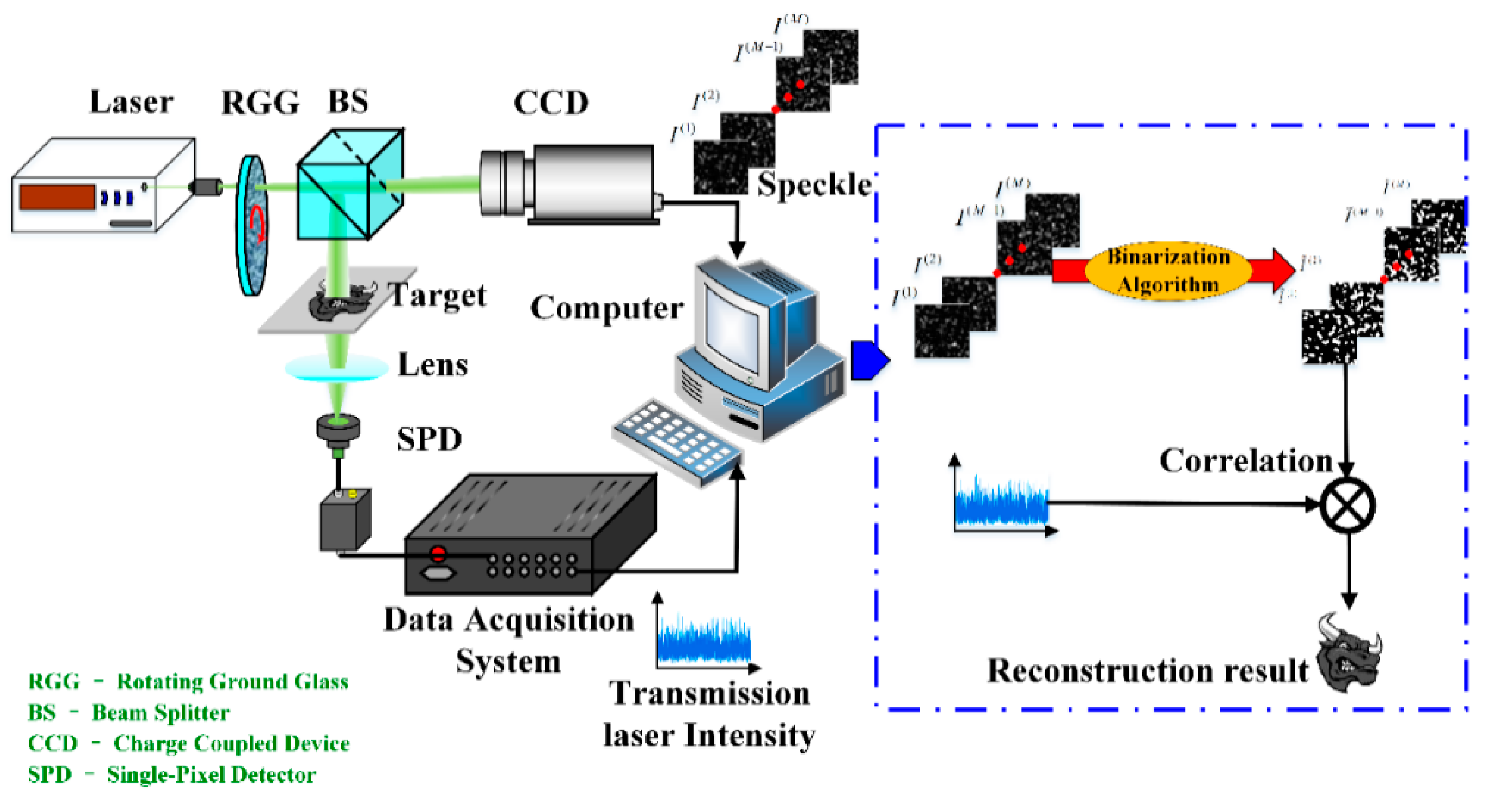
The schematic of BGI system is shown in Figure 1. As Figure 1 shows, the beam emitted from the laser source is illuminated on a rotating ground glass (RGG), which can generate the dynamic speckles to simulate the pseudo-thermal light source. Following the RGG, a beam splitter (BS) is placed in the optical path to split the light into two different optical paths, which are the reference optical path and object optical path, respectively. In the reference optical path, the beam propagates freely, and the spatial distributions of the beam are recorded by a charge coupled device (CCD). The CCD transmits the recorded speckle spatial distribution information to the computer for subsequent processing. In the object optical path, the split beam illuminates on the target. In order to guarantee the speckle spatial distribution recorded by the CCD in the reference optical path is the same as that illuminating the target in the object optical path, the distance from the laser source to the CCD equals that between the laser source and target. A lens is located behind the target to focus the light passing through the target on the active area of the single-pixel detector (SPD). The SPD is connected to a data acquisition system to measure the total transmitted laser intensity. The obtained intensity results are also sent to the computer to reconstruct the image of the target. Here, the kth speckle intensity distribution measured by CCD is denoted as I^(k)(x, y) and the total transmitted light intensity recorded by SPD is denoted as b(k). Therefore, the target transmission distribution can be calculated through the correlation operation between the two detectors. In order to enhance SNR, the reconstruction process utilizes the differential ghost imaging (DGI) technique. The reconstruction can be expressed as:

$$G\left(x,y\right)=\frac{1}{N}{\displaystyle \sum _{k=‘}^N\left(I^{(k)}\left(x,y\right)-\langle I^{(k)}\left(x,y\right)\rangle \right)\left(b^{(k)}-\frac{\langle b^{(k)}\rangle }{\langle O^{(k)}\rangle }{O}^{(k)}\right)},$$

(1)

where O is the total intensity of speckle distribution, and can be expressed as:

$$O^{(k)}={\displaystyle \int I^{(k)}\left(x,y\right)\mathrm{d}x\mathrm{d}y}.$$

(2)

In the BGI system, binary signals with two quantization levels are applied at reference and object optical paths in order to compress the data size. The information recorded by the CCD camera in the reference path is more sensitive to the reconstructed result than that recorded by the SPD in the signal path in the BGI system [35]. Therefore, the binarization algorithm is applied to transform the grayscale speckle images to binary speckle images. The binarization algorithm is the key for the BGI system. The binary speckle obtained by the appropriate binarization algorithm can effectively improve the reconstruction quality of the BGI system. The conventional binarization algorithms adopted in the BGI system include the global binarization algorithm and local adaptive binarization algorithm. In reference [38], the reconstruction results of BGI with different binarization methods are compared. It can be concluded that the reconstruction quality of BGI with local binarization method is relatively higher than that of BGI with global binarization method.

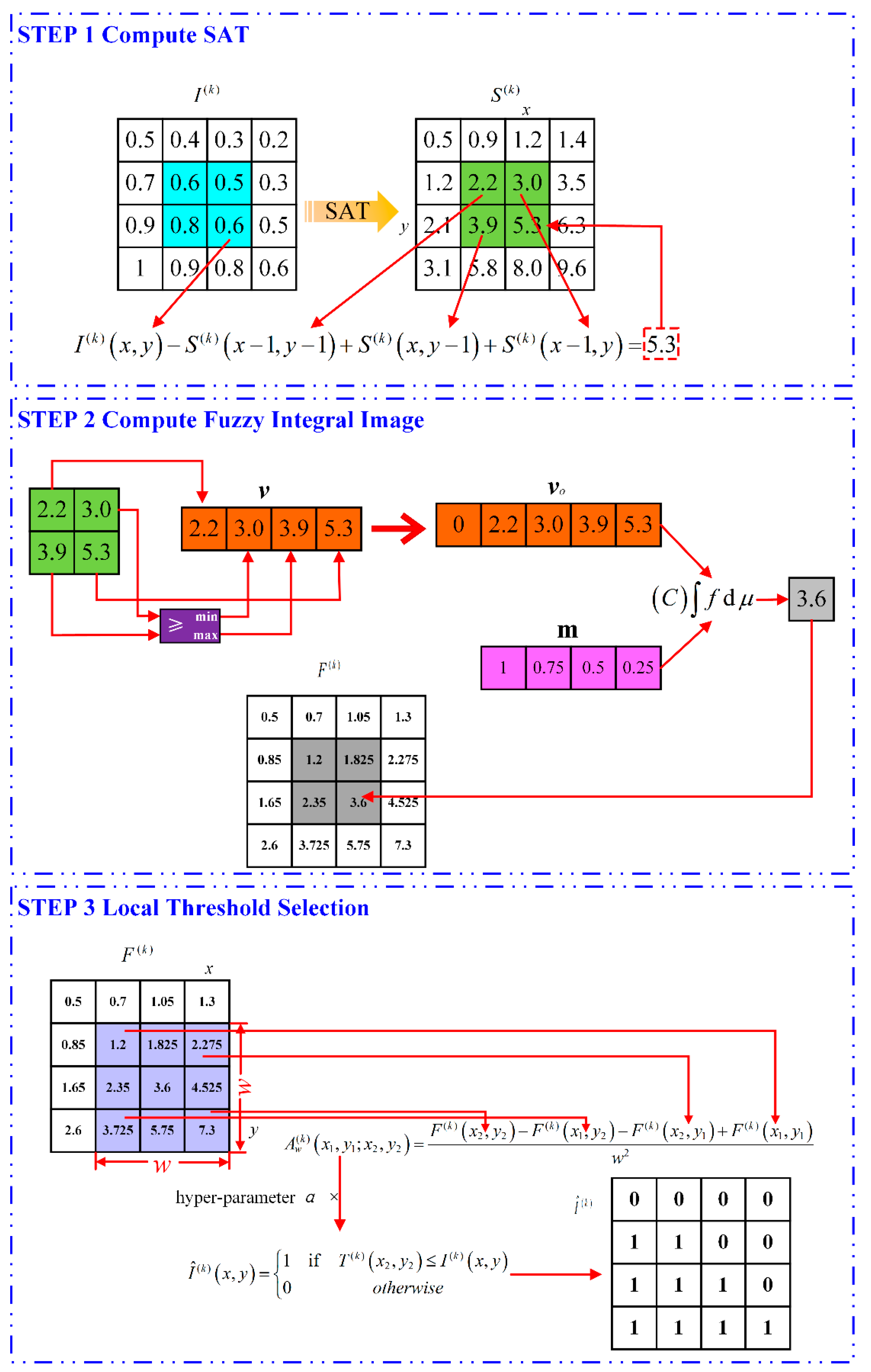
In the proposed method, the Bradley algorithm [46] is modified to select the binarization threshold value. The flow chart of the proposed algorithm is shown as Figure 2. Contrary to the conventional local adaptive binarization methods, such as PPBGI, which calculate the binary threshold pixel by pixel on every speckle image, the proposed method selects the binary threshold according to the fuzzy integral image, which can help avoid uncertainty in binarization and beyond. In addition, the fuzzy integral image is calculated combined with the integral image, which is calculated through the summed-area table algorithm (SAT) [47]. Therefore, the calculation processing of the fuzzy integral image in the proposed method can avoid wasting computational effort in the element sorting.

As shown in Figure 2, Step 1 in the proposed method is to calculate the integral image of each speckle distribution. The integral image has the same dimension as the speckle distribution. For the kth speckle distribution I^(k)(x, y) with r rows and c columns, the numbers of rows and columns of corresponding integral image S^(k)(x, y) are also r and c, respectively. The integral image S^(k)(x, y) is calculated as:

$$S^{(k)}\left(x,y\right)={\displaystyle \sum _{i<x}{\displaystyle \sum _{j<y}{I}^{(k)}\left(i,j\right)}}.$$

(3)

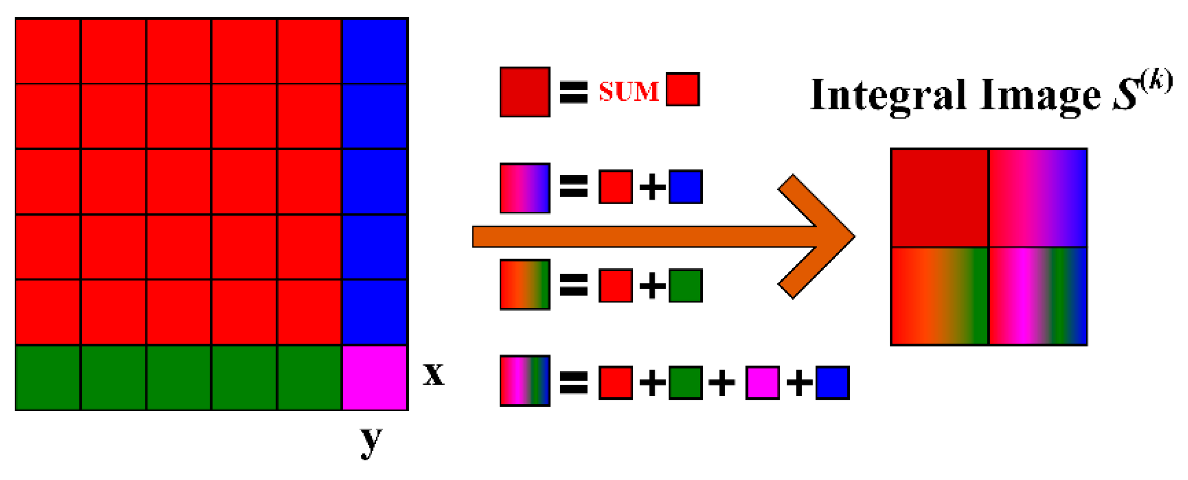
In order to reduce the computational complexity of the integral image, the SAT algorithm is used, which is essentially a recursive algorithm. The schematic of the computation of SAT is shown in Figure 3. As Figure 3 shows, the speckle distribution is divided into four areas highlighted in red, blue, green, and pink. The pixel in the lower right corner of speckle distribution is denoted as (x, y). Therefore, the summed values of different area can be expressed as:

$$\{\begin{array}{c}Su{m}_{red}={\displaystyle \sum _{i<x-1}{\displaystyle \sum _{j<y-1}{I}^{(k)}\left(i,j\right)}}\\ Su{m}_{green}={\displaystyle \sum _{i=x;j<y-1}{I}^{(k)}\left(i,j\right)}\\ Su{m}_{blue}={\displaystyle \sum _{i<x-1;j=y}{I}^{(k)}\left(i,j\right)}\\ Su{m}_{pink}=I^{\left(k\right)}\left(x,y\right)\end{array}.$$

(4)

According to the definition of the integral image, the value of the integral image at position (x − 1, y − 1), (x − 1, y), (x, y − 1), and (x, y) can be, respectively transformed as:

$$\{\begin{array}{l}{S}^{\left(k\right)}\left(x-1,y-1\right)={\displaystyle \sum _{i<x-1}{\displaystyle \sum _{j<y-1}{I}^{\left(k\right)}\left(i,j\right)}}\hfill \\ S^{\left(k\right)}\left(x-1,y\right)={\displaystyle \sum _{i<x-1}{\displaystyle \sum _{j<y-1}{I}^{\left(k\right)}\left(i,j\right)}}+{\displaystyle \sum _{i<x-1;j=y}{I}^{(k)}\left(i,j\right)}\hfill \\ S^{\left(k\right)}\left(x,y-1\right)={\displaystyle \sum _{i<x-1}{\displaystyle \sum _{j<y-1}{I}^{\left(k\right)}\left(i,j\right)}}+{\displaystyle \sum _{i=x;j<y-1}{I}^{(k)}\left(i,j\right)}\hfill \\ S^{\left(k\right)}\left(x,y-1\right)={\displaystyle \sum _{i<x-1}{\displaystyle \sum _{j<y-1}{I}^{\left(k\right)}\left(i,j\right)}}+{\displaystyle \sum _{i<x-1;j=y}{I}^{(k)}\left(i,j\right)}+{\displaystyle \sum _{i=x;j<y-1}{I}^{(k)}\left(i,j\right)}+I^{\left(k\right)}\left(x,y\right)\hfill \end{array}.$$

(5)

Substituting Equation (4) into Equation (5), the following results can be obtained:

$$\{\begin{array}{l}{S}^{\left(k\right)}\left(x-1,y-1\right)=Su{m}_{red}\hfill \\ S^{\left(k\right)}\left(x-1,y\right)=Su{m}_{red}+Su{m}_{blue}\hfill \\ S^{\left(k\right)}\left(x,y-1\right)=Su{m}_{red}+Su{m}_{green}\hfill \\ S^{\left(k\right)}\left(x,y-1\right)=Su{m}_{red}+Su{m}_{green}+Su{m}_{blue}+Su{m}_{pink}\hfill \end{array}.$$

(6)

By solving the Equation (6), the value of the integral image at the position (x, y) is:

$$S^{(k)}\left(x,y\right)=I^{(k)}\left(x,y\right)+S^{(k)}\left(x,y-1\right)+S^{(k)}\left(x-1,y\right)-S^{(k)}\left(x-1,y-1\right),$$

(7)

which specifies {S^(k)(x, y) = 0| x = 0 or y = 0}.

Secondly, the fuzzy integral image F^(k)(x, y) can be calculated based on the integral image S^(k)(x, y). As Step 2 shows in Figure 2, for calculating the fuzzy integral value of the position (x, y), the values in the green box of integral image should be picked out and transformed to an ordered vector v = [v₁, v₂, v₃, v₄], where v₁ ≤ v₂ ≤ v₃ ≤ v₄. According to the property of integral image S^(k)(x, y), it can be seen that the minimum value of the green box is located at the left upper corner, and the maximum value of the green box is located at the right lower corner. Hence, v₁ = S^(k)(x − 1, y − 1) and v₄ = S^(k)(x, y). For further sorting, S^(k)(x, y − 1) is compared with S^(k)(x − 1, y) in order to set the maximum value to v₃ and the minimum value to v₂. By convention, an element 0 is added before the vector v to form the final sorted vector v_o. Moreover, in order to calculate the Choquet integral, the fuzzy measure vector m should be obtained as follows:

$$m=\left[\mu \left(E_1\right),\mu \left(E_2\right),\mu \left(E_3\right),\mu \left(E_4\right)\right].$$

(8)

Here, E_i = {v_i, …, v₄}, I = 1, …, 4 is the subset of vector v, and μ is assumed to be the symmetric fuzzy measure. The vector v is a finite set, and the power set of v is denoted as $𝒫$(v). Therefore, a set function μ: $𝒫$(v) → [0, 1] defined on the power set $𝒫$(v) is a fuzzy measure, if the following conditions are satisfied:

(CC1)

Boundary condition: μ(Ø) = 0, μ(v) = 1;

(CC2)

(Monotonicity: A⊆B ⇒ μ(A) ≤ μ(B) for ∀ A, B ∊ $𝒫$(v);

Additionally, due to the assumption of symmetric fuzzy measure, another condition should also be satisfied:

(CC3)

|A| = |B| ⇒ μ(A) = μ(B) for ∀ A, B ∊ $𝒫$(v).

In the condition of CC3, the |E| represents the cardinal number of the set E. It is further assumed that μ is a uniform fuzzy measure, which satisfies the symmetric fuzzy measure condition, and hence μ can be expressed as [48]:

$$\mu \left(E\right)=\frac{\left|E\right|}{4}.$$

(9)

According to the expression of Equation (9), the fuzzy measure can be calculated as

Table 1. The value of uniform fuzzy measure table.

Set	Fuzzy Measure μ	Set	Fuzzy Measure μ
{v1}	0.25	{v1, v2, v3}	0.75
{v1, v2}	0.5	{v1, v2, v3, v4}	1

.

Therefore, the fuzzy measure vector m is [1, 0.75, 0.5, 0.25]. The discrete Choquet integral can be expressed as:

$$\begin{array}{c}\left(C\right){\displaystyle \int f\mathrm{d}\mu }={\displaystyle \sum _{i=1}^n\left(v_i-v_{i-1}\right)\mu \left(E_i\right)}=\left[v_1-v_0\right]m[1]+\left[v_1-v_2\right]m[2]\\ +\left[v_3-v_2\right]m[3]+\left[v_4-v_3\right]m[4].\end{array}$$

(10)

Here, m[i], i = 1,2,3,4 is the ith element in the fuzzy measure vector m. The computed result of Choquet integral is the value of the fuzzy integral image F^(k)(x, y) at position (x, y).

The final step in the proposed method is to utilize the Bradley algorithm based on fuzzy integral images to obtain the binarization threshold of each pixel. In the conventional Bradley algorithm, the size of threshold calculation window w needs to be set in advance. The average value of the integral image in the selected window is calculated as follows:

$$A_w^{(k)}\left(x_1,y_1;x_2,y_2\right)=\frac{S^{(k)}\left(x_2,y_2\right)+S^{(k)}\left(x_1,y_1\right)-S^{(k)}\left(x_1,y_2\right)-S^{(k)}\left(x_2,y_1\right)}{w^2},$$

(11)

where positions (x₁, y₁) and (x₂, y₂) are the upper left corner and lower right corner of the threshold calculation window, respectively. Hence, the binarization threshold value of pixel (x₂, y₂) can be calculated based on the average value and threshold sensitivity hyper-parameter α (in interval [0, 1]), as follows:

$$T^{(k)}\left(x_2,y_2\right)=\alpha \cdot A_w^{(k)}\left(x_1,y_1;x_2,y_2\right).$$

(12)

It should be noted that the integral image is corresponding to the fuzzy integral image, which is essentially the representation of the integral image in the fuzzy measure domain. Therefore, contrary to the conventional Bradley algorithm, the average value in the proposed method is calculated based on the fuzzy integral image, rather than the integral image. S^(k)(x, y) in Equation (11) should be changed to F^(k)(x, y). As Step 3 shows in Figure 2, the size of threshold calculation window w is selected as 3, and the selected calculation window is colored by blue. The values of the four corners of the blue box are chosen to calculate the average value. Based on the average value combining the hyper-parameter α, the threshold of (x, y) can be finally obtained. The kth binarization speckle is denoted as Î^(k)(x, y) and it is described as follows:

$${\widehat{I}}^{(k)}\left(x,y\right)=\{\begin{array}{cc}1& \begin{array}{cc}\mathrm{if}& T^{(k)}\left(x_2,y_2\right)\le I^{(k)}\left(x,y\right)\end{array}\\ 0& otherwise\end{array}.$$

(13)

After the proposed binary algorithm, the binarization speckles ${\widehat{I}}^{(k)}\left(x,y\right)$ can be submitting into Equation (1) and the final BGI reconstruction result is expressed as:

$$G\left(x,y\right)=\frac{1}{N}{\displaystyle \sum _{k=‘}^N\left({\widehat{I}}^{(k)}\left(x,y\right)-\langle {\widehat{I}}^{(k)}\left(x,y\right)\rangle \right)\left(b^{(k)}-\frac{\langle b^{(k)}\rangle }{\langle {\widehat{O}}^{(k)}\rangle }{\widehat{O}}^{(k)}\right)},$$

(14)

where Ô^(k) = ∫Î^(k)(x, y)dxdy.

Next, the computation complexity of the proposed reconstruction algorithm is analyzed. The number of measurements is denoted as M, which means that M different speckle distributions with the pixel number N are needed for reconstruction. In each speckle distribution binarization process, the first step is to compute SAT for each pixel of speckle distribution. Therefore, the time complexity of the first step is O(N). The second step is to compute fuzzy integral image and only the 4 operative window corners are considered at a time, O(4), leaving the time complexity polynomial in time. Hence, the time complexity of fuzzy integral image computation is O(N) + O(4) + … = O(N). In the local threshold computation process, it is necessary to compute the threshold for each pixel, and the computational complexity of this process is also O(N). Therefore, the overall time complexity of binarization process for M speckle distributions is O(MN). In the target reconstruction process, the reconstruction method is shown in Equation (11), the computational complexity is O(MN). Based on the time complexity analysis of speckle distribution binarization process and the target reconstruction process, the time complexity of the whole proposed algorithm is O(MN).

3. Experiment Results and Comparative Analysis

The experiment conducted based on the schematic of the BGI system as Figure 1 verifies the feasibility of the proposed algorithm. In the experiment, a pulse laser (NPL52B) is chosen as the laser source. The center wavelength and the pulsed average power of the laser are 520 ± 10 nm and 12 mW, respectively. The laser illuminates a ground glass, which is slowly rotated by a stepping motor. A 50%–50% BS (BS031) is behind the RGG to split the light into object and reference paths. In the object path, a transmission spatial light modulator (SLM) is placed following the BS. The computer sends the image of target to the SLM to mimic transmission object. The effective active pixel number of SLM is 1024 × 1024 and the resolution of target image is set to 128 × 128. The diameter of focusing lens is 50 mm and the focus length of the lens is 100 mm. Light transmitted through the target is recorded by a single pixel detector (DET36A2). The detector is connected to a data acquiring card (NI-PXI-5154) to measure the total light intensity. The data acquiring card has 2 GHz bandwidth and the sampling frequency is 5 GHz/s. In the reference path, a CCD (MV-CA050-20UM/UC) is used to record the speckle distribution. The distance between the CCD and BS should equal to that between the SLM and BS. The recorded speckle distributions are all binarized in the computer with the proposed binary method. The intensity distribution information of the target can be obtained by the correlation operation between the binarization speckle and the total light transmitting through the target.

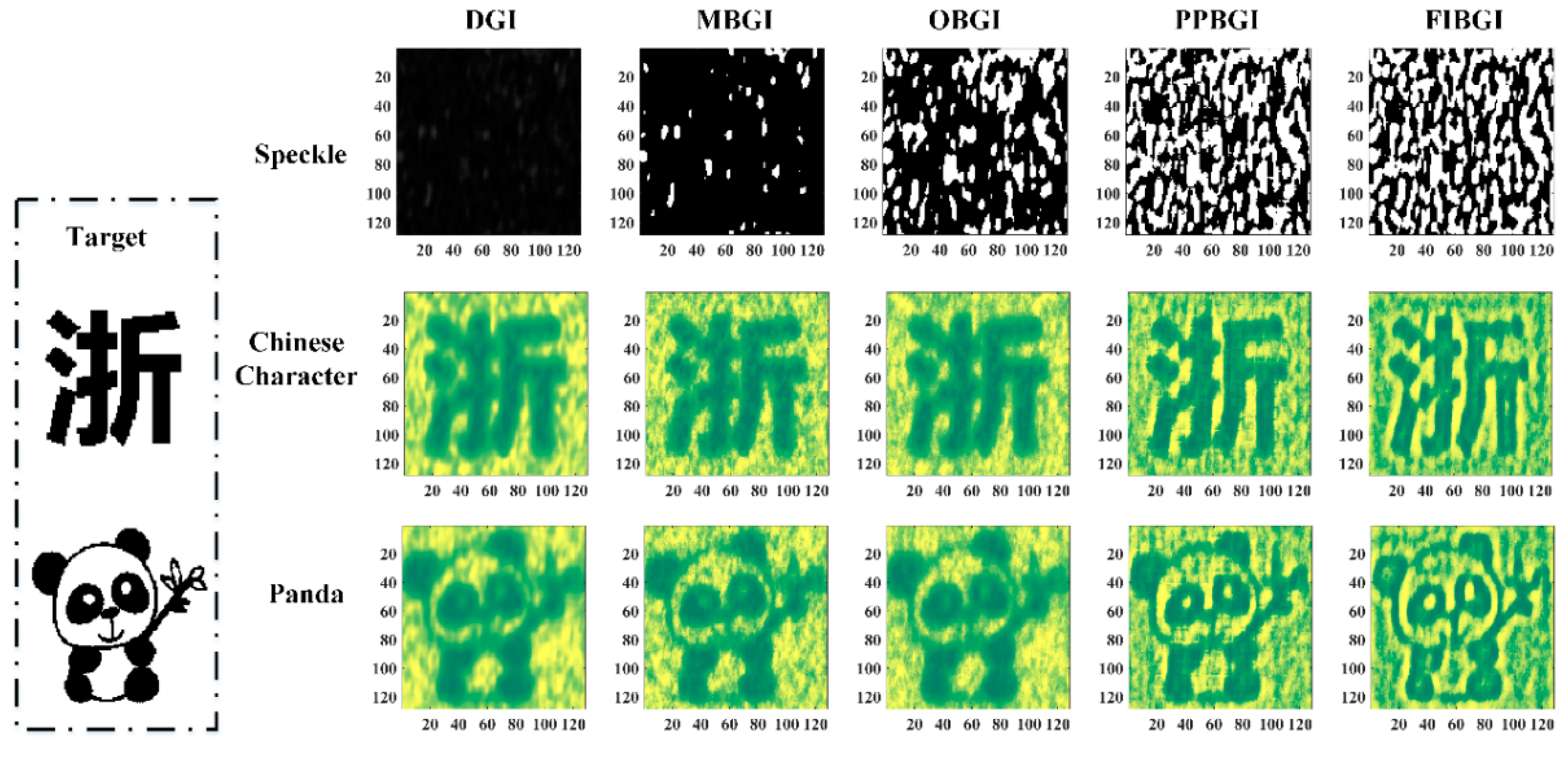
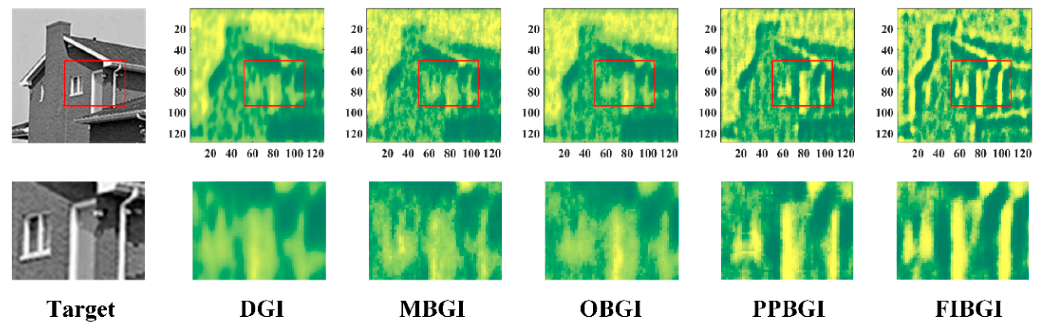
In the experiment, binary images are chosen as the target, whose pixel values are either 0 or 1. The resolution of the targets is 128 × 128. The selected two binary image targets are a Chinese character and panda. The total number of measurements is set to 10,000 and the hyper-parameters w and α are set to 16 and 0.095, respectively. Meanwhile, the reconstruction result of the proposed method is compared with DGI, MBGI, OBGI, and PPBGI. The images in the first row of Figure 4 are the speckle distributions utilized in the reconstruction processing of different methods. The speckle distribution in the first column is recorded by the CCD camera. The speckle distributions of other columns are obtained by different binarization methods. The reconstruction results of different methods are shown in the second and third rows. As the reconstruction results shown in Figure 4, reconstruction results with MBGI and OBGI, which utilize the global binarization method, have the worst image quality. The reconstructed Chinese character and panda image are blurry, with very low resolution and high noise. The reconstruction result of DGI is better than those of MBGI and OBGI. Although the resolution of reconstructed result is still low and the visual effect is still blurred, the noise in the background is reduced to a certain level. From the perspective of visual effect, the reconstructed results of PPBGI and FIBGI, which utilized the local adaptive binarization method, have the best reconstruction effects. Both methods have higher imaging resolutions and clearer target details than the other three methods. Compared with the PPBGI method, the proposed method is better. The edges of the reconstructed image by the PPBGI method are still blurred, and some details of the reconstructed image are distorted.

In order to compare the reconstruction quality of different methods quantitatively, the peak signal-to-noise ratio (PSNR) and structural similarity (SSIM) are calculated as follows:

$$PSNR=10\times {\log }_{10}(\frac{MA{X}_I^2}{MSE}),$$

(15)

$$SSIM(x,y)=\frac{(2{\mu }_x{\mu }_y+c_1)(2{\sigma }_{xy}+c_2)}{({\mu }_x^2+{\mu }_y^2+c_1)({\sigma }_x^2+{\sigma }_y^2+c_2)}.$$

(16)

In Equation (15), MAX_I is the possible maximum value of the image pixels. The reconstructed results with different methods are normalized to the interval between 0 and 1. Therefore, the maximum value of image pixels is 1, namely MAX_I = 1. MSE is the mean square error of the image. For the target image with the pixel number of N = n × m, the MSE is defined as:

$$MSE=\frac{1}{nm}{\displaystyle \sum _{i=1}^m{\displaystyle \sum _{j=1}^n{\left|O\left(i,j\right)-R\left(i,j\right)\right|}^2}},$$

(17)

where O(i, j) represents the target, R(i, j) represents the reconstructed image, and i, j represent the horizontal and vertical coordinates of pixels, respectively. In F (16), μ_x and μ_y are the means of total pixels in the original image and reconstructed image, respectively. σ_x² and σ_y² are the variances of the original image and reconstructed image, respectively. σ_xy is the covariance of the original image and recovered image. c₁ and c₂ are two small positive numbers, which are used to avoid being divided by 0. These two small positive numbers can be calculated as following [49]:

$$c_i={\left(K_{i}L\right)}^2,$$

(18)

where I = 1, 2, K_i << 1 is a small constant, and L is the dynamic range of the pixel values, which is 1 for normalized image. According to the analysis in reference [49], K_i can be selected arbitrarily, and the performance of the SSIM index algorithm is fairly insensitive to variations of these values. Therefore, following the reference [49], K₁ and K₂ are also set as 0.01 and 0.03 in the SSIM index calculation, respectively. The two small positive numbers c₁ and c₂ are 10⁻⁴ and 9 × 10⁻⁴, respectively.

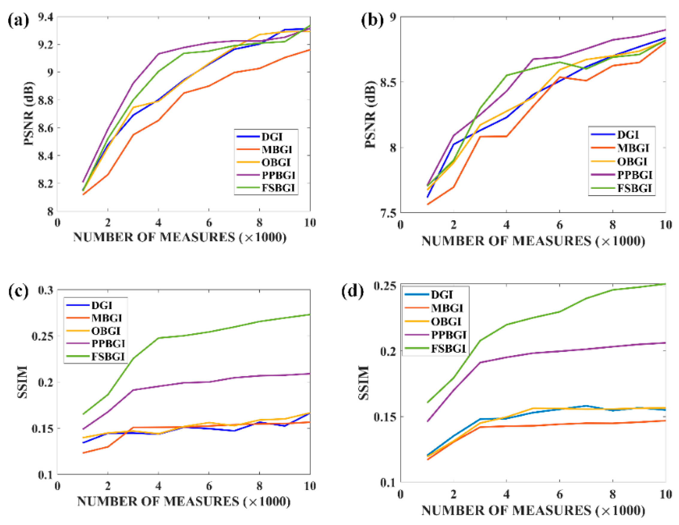
The calculated results are shown in Figure 5. Figure 5a–d are the PSNR of reconstructed Chinese character, PSNRs of reconstructed panda, SSIMs of reconstructed Chinese character, and SSIMs of reconstructed panda, respectively, with every method under different sampling rate conditions. The horizontal coordinate of each sub-image in Figure 5 represents the number of measurements, which range from 1000 to 10,000. The vertical coordinate represents the value of quantitative evaluation index. In Figure 5, different colors of curves represent different reconstruction algorithms. As Figure 5 shows, the number of measurements affects the reconstruction quality of all the algorithms. The PSNR and SSIM of all the methods improve with the increase in measurement numbers. It can be concluded from Figure 5a,b that the PSNRs of the reconstructed results by different methods have little difference under the same number of measurements. The PSNR of the proposed method does not exceed those of other methods, and sometimes it is even lower than those of other methods. The reason for this is that the noise in the background is relatively high, although the reconstructed result of the proposed method has a better resolution. The higher the noise is in the background, the bigger the error between the reconstructed results and corresponding pixel points of the original image is. Therefore, the PSNR of the proposed method has no significant difference with other methods, whereas there is a deviation between the quantificationally calculated PSNRs and visual effect. Contrary to the PSNR, the SSIM is more highly consistent with visual effects. From the perspective of image composition, the SSIM defines structural information as an attribute that reflects the structure of objects in the scene. Additionally, the attribute is independent of brightness and contrast. Distortion is modeled as the combination of three different factors: brightness, contrast, and structure. The three factors are estimated by the mean value, standard deviation, and covariance, respectively. The SSIM focuses more on the evaluation of image similarity, and the evaluation accuracy of image similarity is better than PSNR [49]. As Figure 5c,d show, The SSIMs of the reconstructed results by the local adaptive binarization methods (PPBGI and FIBGI) are higher than those by other methods (OBGI, MBGI, and DGI). Moreover, compared with the PPBGI, the proposed method is better. When the number of measurements is small, the SSIM of reconstructed results with the proposed method is relatively low, but still higher than other algorithms. With the increase in measurement numbers, the SSIM of the proposed algorithm improves rapidly and remains optimal.

In addition, a grayscale image is selected as the experimental target to verify the superior reconstruction ability of the proposed method. A grayscale house image is selected as the target. The resolution of the selected grayscale image is 128 × 128. The number of measurements is 10,000. The reconstructed results with different methods are shown in Figure 6. The images in the first row of Figure 6 are the selected target and reconstructed results with various methods. Similar to the case of binary target, the result reconstructed by the proposed method has the best overall visual effect. The resolution of the reconstructed result with the FIBGI is better than those with other methods. To make the contrast more obvious, the reconstructed result in the red rectangular area is enlarged and shown in the second row of Figure 6. 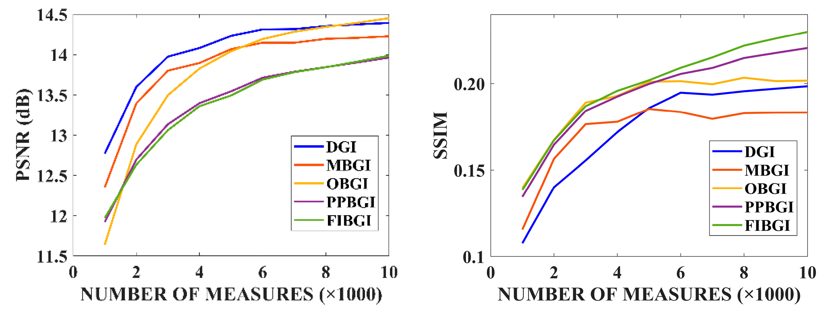It can be seen from the second row of Figure 6 that much detail information is lost in the reconstructed results with DGI, MBGI, and OBGI. The window frame, the edge of the wall and the water pipeline look blurry. Although some outline information of these regions can be seen in the results reconstructed by the PPBGI method, the resolution is still not high. Especially, there is a slight checkerboard artifact in the reconstruction result of the PPBGI. In comparison, the result reconstructed by the proposed method has the highest image quality. The detail of the reconstructed image is relatively clear and obvious compared with the global binarization methods, such as MBGI and OBGI, and there is no checkerboard artifact compared with the PPBGI method which also adopts local adaptive binarization method. The PSNR and SSIM of the reconstructed results of grayscale target are also calculated and shown in Figure 7. As Figure 7 shows, similar to the binary target, the PSNRs and SSIMs of all the methods improve with the increase in the number of measurements. The PSNRs of the local binarization methods are lower than those of the global binarization methods at different measurements, as there is more noise in the reconstruction results with the local binarization methods. The reconstructed result of the proposed method performs well in SSIM. When the number of measurements is low, the SSIMs of the reconstruction results of different methods are relatively low, and there is little difference between each other. With the increase in the number of measurements, the SSIMs of the reconstructed results using various methods improve, and the SSIM of the proposed method has the fastest improving rate. When the number of measurements reaches 10,000, the SSIM of the proposed method has a higher value than the ones of other methods. It can be concluded from the quantitative comparisons that the reconstructed results with global binarization methods and DGI have relatively low noise level, and therefore the PSNRs are high. Although the results reconstructed by local binarization methods have higher noise level, the results are more similar to the target. Hence, the SSIM of reconstruction results with binarization method are higher than those with global binarization methods.

4. Discussion

There are two hyper-parameters, α and w, which influence the reconstruction quality of the FIBGI. In this section, the effects of these two hyper-parameters on the quality of reconstruction will be discussed in detail, and the way to set these two hyper-parameters, when the prior information of the target is unknown based on the discussion results, will be summarized.

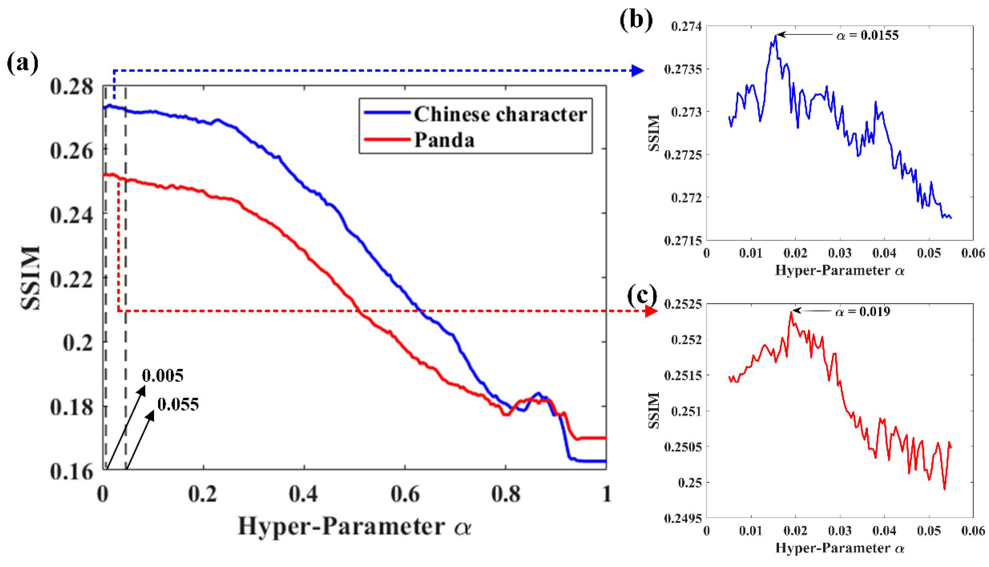
Firstly, the influence of the hyper-parameter α, the threshold adjustment parameter, on the imaging quality is analyzed. When the value of α is close to 1, most of the values in the binarization speckle image are 1. When the value of this parameter is close to 0, most pixel values of the binarization speckle image are 0. The value range of the hyper-parameter is [0, 1]. The exact value needs to be set empirically, or traverse the interval [0, 1], for the best imaging quality. According to the experiment comparison in Section 3, the SSIM is more consistent with the visual effects. Hence, the SSIMs of reconstructed results of the image of a Chinese character and the image of a panda are calculated by increasing the hyper-parameter α from 0.005 to 1 with the step of 0.005 when the number of measurements is 8000, and the hyper-parameter w is set as 10. The calculated SSIMs are shown in Figure 8. The blue line in Figure 8a represents the SSIM of the image of the Chinese character, and the red represents the SSIM of the image of the panda. It can be seen from Figure 8a that the overall trend of SSIMs of the two targets both decrease with the increase in hyper-parameter α. In addition, there is an optimal value in the interval of [0.005, 0.055]. In order to determine the optimal value more precisely, the hyper-parameter increases from 0.005 to 0.055 with the step of 0.0005. The SSIMs of the image of the Chinese character and the image of the panda changing with α in the interval of [0.005, 0.055] are shown in Figure 8b,c, respectively. It is obvious that there is an optimal value existing in the SSIM curve. The optimal values of the images of the Chinese character and panda are 0.0155 and 0.019, respectively. When the hyper-parameter is set to the optimal value, the SSIM of reconstructed result is the maximum. Moreover, it can be concluded that the optimal value of hyper-parameter is not the same for different targets. Therefore, it is not appropriate to choose the same value for the parameter for different targets. Fortunately, there is no significant difference in SSIM when the value of hyper-parameter α is in the interval [0, 0.03]. In the case of low requirements for SSIM, it is feasible to select random value in the interval [0, 0.03].

The influence of the hyper-parameter w on the imaging quality is also analyzed. This parameter determines the size of the local adaptive binarization window. The larger the window is, the more pixels affect the binarization threshold. Especially when the hyper-parameter equals the size of the target, the local adaptive binarization is equivalent to the global binarization. 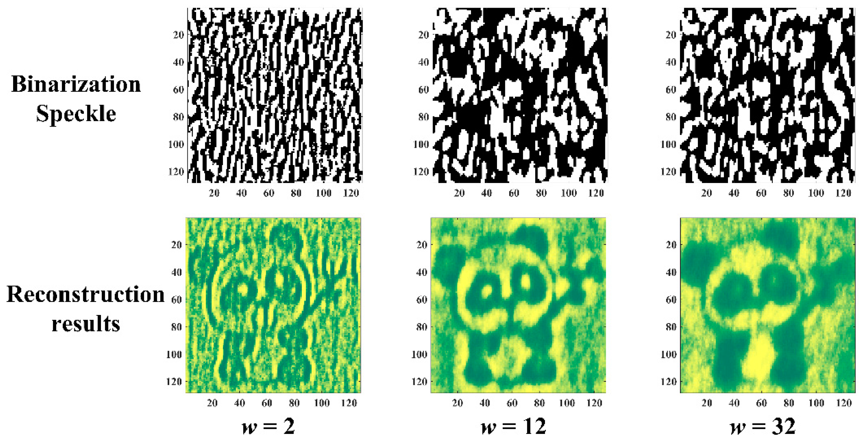Here, the number of measurements is set as 8000, the hyper-parameter α is 0.019, and the hyper-parameter w is selected as 2, 12, and 32, respectively. The reconstruction results of the image of the panda with the proposed method are shown in Figure 9. The first row of Figure 9 is the binarization speckle when the hyper-parameter selects different values. The images in the second row are the corresponding reconstruction results. It can be seen that the binarization speckle has a finer structure when the value of hyper parameter w is relatively small. Therefore, the resolution of the corresponding reconstruction results was higher. However, the signal-to-noise ratio is low, and there is a huge noise in the reconstruction result. With the increase in the hyper-parameter w, the fine structure of the binarization speckle gradually disappears and the resolution of the corresponding reconstruction results decreases. The noise in the reconstruction results is also reduced. Especially when the value of w is large, the visual effect of the reconstruction result with the proposed method is similar to those of other conventional global binarization methods, such as MBGI and OBGI, which indicates that the local adaptive binarization is similar to the global binarization when the local window is too large.

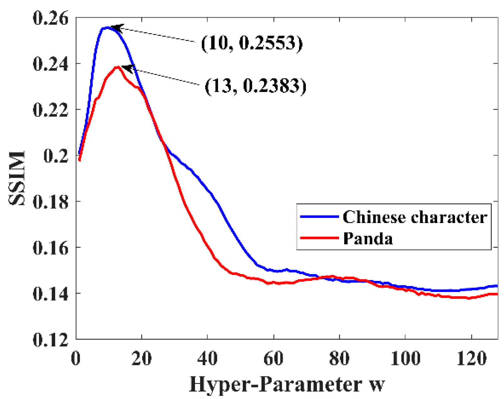
Furthermore, similar to the above analysis of hyper-parameter α, the SSIMs of the image of the Chinese character and image of the panda are calculated when the hyper-parameter w selects different values. The calculated results are shown in Figure 10. It can be seen that there is also an optimal value existing in the curve of SSIM. When the hyper-parameter w selects 10 or 13, respectively, the best reconstruction results of the image of the Chinese character and panda can be obtained. This also means that the contradiction between the noise and resolution of the reconstruction results can be balanced to a great extent when the hyper-parameter w is set to this optimal value.

According to the analysis about hyper-parameters α and w, it can be concluded that the hyper-parameters α should be selected as a relatively small value when the prior information of the target is known. The arbitrary value of hyper-parameter α in the interval [0, 0.03] has little influence on the reconstruction quality. The value selection of hyper-parameter w, which represents the size of local binarization window, should be evaluated according to the requirements of imaging. If the imaging result needs to have a high signal-to-noise ratio, the value of this parameter should be increased as much as possible. If the imaging result needs to have a high resolution and visibility, the value of this parameter needs to be relatively small.

5. Conclusions

Based on BGI system architecture, the FIBGI method is proposed to achieve reconstruction of the target with high quality. Contrary to the conventional binary methods, such as MBGI, OBGI, and PPBGI, the proposed method utilizes the result of fuzzy integrals to determine the binarization threshold. The main structure of the algorithm is the Bradley algorithm, which is a kind of local adaptive binarization algorithm. In the proposed method, the integral image is firstly calculated through the SAT algorithm. According to the integral image, the fuzzy integral image is obtained through the Choquet integral. It is the introduction of fuzzy integrals in the process of binarization that makes the result of speckle binarization more accurate, and retains more speckle information. Finally, similar to the conventional Bradley algorithm, the binarization threshold of each pixel is determined by the calculated fuzzy integral image, threshold sensitivity hyper-parameter α, and the threshold calculation window hyper-parameter w. The effectiveness of the proposed algorithm is verified by theoretical analysis and experiment results. It is compared qualitatively and quantitatively with the DGI, MBGI, OBGI, and PPBGI methods. The proposed method can obtain higher quality reconstruction results than other methods. Although there is noise existing in the reconstruction results of the proposed method, the resolution of the reconstruction result is much higher, and the visual effect is much better. Moreover, the PSNRs and SSIMs of various methods are calculated. Although there is little difference in PSNR among all the methods, the SSIMs of the proposed method are significantly higher than those of other methods with different numbers of measurements. In addition, the influences of the threshold sensitivity hyper-parameter α and the threshold calculation window hyper-parameter w are also analyzed in the paper. Through the analysis, it can be found that there is an optimal value for each hyper-parameter. The best reconstruction results can be obtained when the two hyper-parameters are set to their respective optimal values. In addition, the selection of the threshold calculation window hyper-parameter w needs to be based on the actual imaging requirements. When the image resolution is more important, the parameter can be set to a small value, and when the image signal-to-noise ratio is more important, the parameter can be set to a large value. In the future, the SSIM uncertainty of the reconstruction results with the proposed FIBGI method will be analyzed. A dataset containing grayscale images with different complexities will be built, and the grayscale image in the dataset will be reconstructed with the proposed method. With the reconstructed results, the average and variance of the SSIM will be calculated, and the relationship between SSIM and image information entropy will also be studied.