
s2p: Provenance Research for Stream Processing System


1
The Key Laboratory on Reliability and Environmental Engineering Technology, Beihang University, Beijing 100191, China
2
School of Reliability and Systems Engineering, Beihang University, Beijing 100191, China
*
Author to whom correspondence should be addressed.
Appl. Sci. 2021, 11(12), 5523; https://doi.org/10.3390/app11125523
Submission received: 21 May 2021
/
Revised: 3 June 2021
/
Accepted: 11 June 2021
/
Published: 15 June 2021
(This article belongs to the Collection Big Data Analysis and Visualization Ⅱ)
Abstract
:The main purpose of our provenance research for DSP (distributed stream processing) systems is to analyze abnormal results. Provenance for these systems is not nontrivial because of the ephemerality of stream data and instant data processing mode in modern DSP systems. Challenges include but are not limited to an optimization solution for avoiding excessive runtime overhead, reducing provenance-related data storage, and providing it in an easy-to-use fashion. Without any prior knowledge about which kinds of data may finally lead to the abnormal, we have to track all transformations in detail, which potentially causes hard system burden. This paper proposes s2p (Stream Process Provenance), which mainly consists of online provenance and offline provenance, to provide fine- and coarse-grained provenance in different precision. We base our design of s2p on the fact that, for a mature online DSP system, the abnormal results are rare, and the results that require a detailed analysis are even rarer. We also consider state transition in our provenance explanation. We implement s2p on Apache Flink named as s2p-flink and conduct three experiments to evaluate its scalability, efficiency, and overhead from end-to-end cost, throughput, and space overhead. Our evaluation shows that s2p-flink incurs a 13% to 32% cost overhead, 11% to 24% decline in throughput, and few additional space costs in the online provenance phase. Experiments also demonstrates the s2p-flink can scale well. A case study is presented to demonstrate the feasibility of the whole s2p solution.
1. Introduction
Currently, massive volumes of data are produced and analyzed for better decision-making. In many modern big data scenarios, such as stock trading, e-commerce, and healthcare [1], data have to be processed not only correctly but also promptly. Some data naturally comes as infinite stream and temporal featured, whose value declines rapidly over time [2]. These aspects pose tremendous computational challenges. Distributed stream processing (DSP) thereby receives more significant interest in the light of business trends mentioned above. As a new paradigm in big data processing, DSP is designed to handle a continuous data stream within a short period (i.e., from milliseconds to seconds) after receiving data. Beyond niche applications in which data are handled by traditional stream processing systems, current DSP systems are widely adopted across modern enterprises in complex data computation.
However, like other large system software [3], DSP applications are not always correct and performant for different reasons, including, but not limited to, data corruption, hardware failure, and software bugs. As they increasingly interact directly with the physical environment (e.g., IoT data analysis), their source data are more susceptible to interference (e.g., noise data), malformed data, or error. When some suspicious results come out, it will be necessary to verify their correctness and trace the error chain back to localize the root failure. Keeping data traced and understanding the cause of a suspicious result is especially desirable when a critical situation involving a streaming processing application occurs [4]. This is the first motivation for our stream provenance research to enhance DSPs with the capability to replay some data transformation processes and tracing each relevant data individually. The second motivation is the requirement for data accountability. There are rules such as GDPR [5] imposing obligations on data controllers and processors, where it will be necessary to verify how data was used and transferred without consent violation. The third motivation is about the support for interactive debugging sessions [6,7], where provenance works as the critical part [7].
The basic idea of provenance [8] is to explain how the output results relate to their input data, including the origin and various transformations contributing to the end product. A provenance graph can show the flow of one data routing from source (inputs) to results (outputs). Its initial work started in database areas [9] and later broadened to other areas (e.g., operation systems, big data systems) [10]. Provenance is challenging in the big data area [8], as most traditional provenance solutions require accessing the whole data set, which is hard to satisfy when faced with massive amounts of data. For big data systems, their four Vs (i.e., volume, velocity, variety, and veracity) bring fundamental challenges to provenance; these challenges together are referred to as the “Big Data Provenance” problem [11,12] in the literature. It involves capturing, storing, managing, and querying provenance data. In state-of-the-art solutions for big data systems, provenance annotations are generated for data tuples and all involved intermediate data are passed from source data to each output result. During this process, all source data must be stored temporarily, and those that do not contribute to the interested output result must be discarded later [4]. Intermediate data are required to be maintained when backward and forward tracing are supported in some solutions [13]. Storing and managing these data may not be feasible for many big data applications, since the size of data used for assisting analysis can easily be at a similar level of the input data itself, or multiple times larger than the input data [14] if they are not sophistically managed.
There exist two categories of provenance work that target different data processing paradigms separately (batch processing vs. stream processing); they are shown in Table 1.
For those targeting batch processing systems [15,16], the state-of-the-art solutions include RAMP [17] (for Hadoop), HadoopProv [18] (for Hadoop), and Titian [19] (for Spark). Batch processing systems periodically consume blocks of static data (usually long in hours or even days). They adopt the BSP model [20,21], which processes in a series of supersteps, i.e., iterating a large batch of data followed by a global barrier with synchronization among workers. These two features bring convenience in designing a provenance solution for batch processing systems, as they can conveniently revisit any source data and intermediate data from disks (e.g., for Hadoop) or memory (e.g., for Spark). The BSP model also makes replay from some stages (e.g., Titian [19]) possible, as it naturally divides the job into stages.
On the contrary, solutions targeting stream processing systems include Ariadne [22,23] and GeneaLog [4,24], among other solutions. DSP adopts the dataflow model [25], in which incoming data are processed as soon as they arrive and produce results within a short period (usually in milliseconds or seconds). As a new big data processing pattern, DSP systems present some new features that challenge the provenance design described as follows.
- (1)
- Stream data, a.k.a. real-time data, are ephemeral in many applications, which means that their intermediate data will not be persisted during transformation within jobs. Storing these intermediate data and their provenance metadata naively is impossible because the total data may be multiple times larger than the source data. If we store all dependencies and intermediate data objects, the amount of information recorded can potentially cause a storage burden problem.
- (2)
- Stream processing systems usually generate results within milliseconds to seconds processed by jobs. A heavy provenance capturing mechanism will bring in perceived delay substantially.
- (3)
- Current DSP systems usually closely integrate state with computation [26]. Unlike the batch processing system, in which data is batched and computed as a whole group, stream processing systems lack a similar global view for the whole data set. State in stream processing systems is then used to memorize the historical data ever seen or some intermediate results, which may indirectly affect the results. Due to this new feature, a consummated provenance for stream processing systems should also consider how states evolve together with the data transformation.
We usually have no previously known information about which kinds of data are biased or more likely to be tracked by users, whether in crash-culprit scenarios or accountability purposes. This elicits another requirement, i.e., the ability to track every piece of stream data in a provenance solution. It is extremely inefficient to process the entire data set on every tuple, especially when the data is large. However, provenance for intermediate data is not directly used most of the time [14], which means that retaining full provenance for every piece of data would be a waste for most cases. In some scenarios, users want to “replay” intermediate data in detail [1]. In other scenarios [4,24], they may only need to know which specific source data contribute to the results to be analyzed.
We present s2p, a novel provenance solution for DSP systems to tackle the challenges above. The s2p solution consists of online provenance and offline provenance, through which the previous one builds the mapping relation between source data and result data, and the latter provides detailed information about transformation processes, intermediate results, and more. This design is inspired by the philosophy of lambda architecture [27] in which different results with different precision are handled by different process. Our s2p solution traces stream data across varieties of operators. We consider the semantics of each operator (e.g., map, filter, etc.) when deciding the relationship among data, but we leave the user-defined logic in UDFs as backboxes. We augment each operator to propagate provenance metadata (e.g., UUID of data) with each stream data. We implement s2p by modifying the DSP framework and extending its runtime to propagate provenance data. Our s2p is transparent to users without any additional modification to the original program. Using s2p, we can exploit the detailed provenance information of the interested stream data only.
In addition, s2p can achieve high performance by: (1) only replying from some specific point that is close to the computation process for target data, (2) parallelizing the replay process on a cluster, (3) caching the most frequent queried data sets for fast further access, and (4) building provenance graph asynchronously and stopping the replaying process once necessary provenance information for target data is obtained.
In our study, we have built a prototype to materialize the main features of s2p and designed experiments to quantify its side effect on normal DSP system execution. We also carried out one case study to show the feasibility of s2p.
In summary, the main contributions of this paper are:
- s2p, a novel provenance solution for stream processing systems that combines offline and online parts and provides fine- and coarse-grained provenance at a level of precision supported by few existing DSP provenance systems.
- Previous approaches aim for all input data oriented provenance analysis; however, it is hard to support detailed provenance analysis at the tuple level. On the contrary, our solution targets detailed provenance for a small amount of stream data by replaying the computation process and merely monitoring the interested data.
- Our solution considers state transformation of stateful operators together with the data transformation process in provenance analysis, whereas few existing DSP provenance systems take operator states into account.
- To minimize the data transformation burden to the network, we manage our provenance data locally and only aggregate some chosen data when a provenance query happens.
- One prototype s2p-Flink is built on Apache Flink [28] to demonstrate the solution of s2p.
- We conduct experimental evaluations with three subject applications. Results show the s2p scaling to large data sets with acceptable overhead.
- One case study is to show its feasibility.
The remainder of the paper is organized as follows. Section 2 contains a brief overview of DSP, the DSP provenance problem definition, and a short introduction to Apache Flink. Section 3 provides a framework for how s2p works. Techniques involved during online provenance are introduced in Section 4, and offline provenance-related ones are introduced in Section 5. Section 6 describes how we manage and query provenance data. The experimental evaluation is presented in Section 7. The case study is included in Section 8. Related works about solving big data provenance problems are presented in Section 9. We conclude with a summary and discussion of future work in Section 10.
2. Preliminaries
We start with a brief overview of the stream processing paradigm accompanied by a unified DSP computing model and how it is executed. Then, we define DSP provenance problems with an overview of the challenges they meet. At last, we introduce Apache Flink, which is selected as the object system in our research.
2.1. DSP System Model
According to Russo et al. [35], DSP is the key to process data in a near real-time fashion, which processes the incoming data flow on multiple computing nodes. Several DSP systems have been developed and applied in industry, including Storm [36], Samza [37], and Flink [38], among others. DSP systems achieve low latency and high throughput by processing the live, raw data as soon as they arrive. Meanwhile, DSP systems usually perform message processing without having a costly storage operation [39]. It is also required to handle stream imperfections such as delayed, missing, and out-of-order data [40].
DSP applications execute in a parallel fashion with numerous subtasks that process some partition of data. One DSP usually consists of UDFs, which are first-order functions plugging into second-order functions (i.e., DSP APIs provided by different DSP frameworks such as flatmap).
A DSP application (a.k.a. job) represents a data processing pipeline in which operators are sophisticatedly chained together as DAG and data transformations are conducted inside the operators. From the developers’ view, one typical DSP application is the composition of some set of DSP APIs and user-defined logic within them. As shown in Figure 1, DSP APIs, through which we can interact with DSP operators, and user-defined logic are two blocks for one DSP application. DSP applications are usually compiled and expressed in graph views. Then, these graphs are submitted to clusters working with the DSP runtime. DSP applications are automatically scheduled and executed by the DSP runtime environment.
During execution, operators, which are the basic units of one data processing pipeline, are split into several parallel instances in a distributed environment with instances deployed and executed on different nodes.
This paper adopts a unified DSP computing model, as the example in Figure 2 shows, to demonstrate our methods more conveniently.
DSP jobs are deployed at multiple nodes and each operator (if its parallelism is set more than one) is split into multiple parallel instances. The stream manager collects processing information periodically. Nodes in Figure 2 are named with different naming conventions (e.g., Task Manager in Flink [28], Worker in Apache Storm [36]). Those instances are deployed in nodes. Processing nodes refer to physical machines, containers, virtual machines, etc. For reducing data buffer and transition traffic purposes, multiple operators may be chained together and run on a single processing node. For the fault tolerance purpose, stateful operators will update their state remotely to the stream manager periodically.
DSP’s computing model consists of source operators that receive steam data from various sources, transformation operators, and sink operators that emit the final results. DSP also defines window operators on the infinite stream to cope with stream data’s unbounded nature by grouping them into chunks. Windows can be time-based, which decomposes the stream over time, or count-based, which divides the stream by the number of data already included in the window.
Operators in DSP can be stateless or stateful. Stateless operators are purely functional, which means that their output is solely dependent on their input. However, for stateful operators, their output results depend on their input and internal state over the historical stream data. Most DSP applications will contain one or more continuous operators to process data in a long-running fashion [41]. Since data are streamed and arrived over time, many nontrivial operators must memorize records, partial results, or metadata, which are also known as state handling (i.e., remerging past input and using them to influence the processing of future input) in the DSP systems. These stateful operators receive stream data, update their internal state, and then send new stream data.
2.2. Stream Provenance Problem Definition
The purpose of DSP provenance is to track how each stream data has changed over time. The provenance schema involves provenance capturing, storage, and querying. Here, we will classify some related expressions for future convenience. The set represents the input stream data into one operator with timestamps , etc. The set represents the computing results out of this operator with timestamps , etc. is operator transformation, which encapsulates user-defined data processing logic.
Then, we conduct the provenance definition in this paper. Result data ’s provenance consists of the minimal source data set and a series of transformations that derivate it from the source data set. In other words, the provenance for stream result data is constituted by subinstance of source data where the set I is the minimum set among all subsets that contribute to , and transformations such that .
Though user-defined data processing logic varies, the semantics of DSP APIs constrain the input and output data relationship at a high level. For instance, map is a standard operator in DSP systems that ingests one stream data each time and produces one output. In this case, corresponds to map. For any output data , we can find at least one input . Hence, we can express the provenance for the result data as , where is the minimal subset of the input data that leads to .
However, the way to find the minimal set I for one DSP system differs for stateless operators and stateful operators. For stateless operators, their output results purely depend on the latest input and operators’ semantics. Nevertheless, for stateful operators, the historical stream data will also potentially contribute to the current result indirectly through the internal states S, which are persisted by stateful operators. Consider one DSP job (shown in Figure 3) as an example. It consists of three stateless operators (i.e., , , ) and one stateful operator (i.e., ). We can see that ’s output is determined by its input values and its “side effects” (i.e., state) affected by historical data.
To include complete provenance information for stateful operators, we express it as a list of nested tuples , where is the minimal subset of input data. The state is a snapshot when is being processed and potentially decided by the historical input data recursively. For the example in Figure 3, we express the provenance of one result data as a graph, shown in Figure 4.
Because of the long-running (e.g., months, or even years) nature of one nontrivial DSP job, recording all state transition for further provenance purposes is expensive or even impossible. In this paper, our solution will only pinpoint every state transition in a certain period in the offline provenance phase when quite a few state data are to be stored.
State tracking is not the only obstacle for DSP provenance. DSP data’s ephemeral nature brings another problem: that we have to cache the intermediate stream data for further provenance query. Since we have no previously known information about the potential analysis bias in the future, we have to assume that every stream data might be selected as object data. Therefore, our solution should have the capability to retrospect every piece of data. Our first attempt to achieve this requirement is to cache all the intermediate data before and after every operator. However, we ran into two significant issues, i.e., enormous space cost and rapid decline in DSP response time.
Space cost: The space cost for storing all intermediate data is prohibitively expensive. We implement this cache-all mechanism in Apache Flink, called Flink-cache-all afterward and assess how much additional space is required to store intermediate data. Flink-cache-all is instrumented to collect data before and after each operator. This instrumentation wraps operators and sends a copy of every data item to our provenance manage system. Figure 5 shows a quantitative result about additional space needed to execute the WordCount job in Flink-cache-all under different workloads. In general, the size of the intermediate data increases proportionally with the size of the workloads. More specifically, the intermediate data size is about 5.3 times the size of the source data. The storage cost is relatively expensive, let alone more provenance metadata required to store for a fully functional provenance system.
Response time: Data copy happens locally since our provenance manage system is distributing alongside each node. In our experiment, it takes about three milliseconds on average to send one piece of data item to the provenance manage system. We found that the execution time of our experimental job on Flink-cache-all is over 1000 times as much as on normal Flink (e.g., Flink-cache-all takes 1316 seconds in total to process a 20 MB data set while it finishes within 1 second for normal Flink accordingly).
In summary, we have clarified our provenance concept for DSP systems. We also have analyzed challenges in designing DSP provenance with a quantitative assessment of additional space and time needed when naively caching all intermediate data.
2.3. Apache Flink
In this paper, we implement s2p on Flink, a leading stream processing system with increasing popularity. It is an emerging stream processing engine that follows a paradigm that embraces continuous data stream processing as the unifying model for real-time analysis and batch processing [28].
Flink executes dataflow programs in a data-parallel and pipelined manner [42]. Flink applications can be implemented in various program languages (e.g., Java, Scala, etc.), and then automatically transformed into dataflow programs executed in clusters. A dataflow starts with one or more sources and ends in one or more sinks, represented as DAG under specific conditions.
3. DSP Provenance
This section will briefly talk about our provenance solution in tackling DSP provenance problems. As shown in Figure 6, our solution consists of online provenance for coarse-grained solutions, offline provenance for fine-grained solutions, and provenance management to handle all provenance data.
Online provenance is to build the mapping relationship between source data and result data, i.e., what are all combinations of source data that contribute to the output results after executing the application. Operator intrusion is required with introspecting operators in DSP systems to capture data relationships before and after each transformation. Nevertheless, it lacks a detailed description of how inner transformation happens during stream data passing through operators.
As a supplement to online provenance methods, offline provenance refers to capturing the data transition process in detail, which, no doubt, is much heavier. Our offline solution isolates with the original execution environment by replaying specific data transformation in a simulated environment, which is more controllable and on a smaller scale.
We also present how to manage provenance-related data in online and offline phases and respond to the provenance query.
4. Online Provenance
The online provenance phase aims to build the relationship between each output result data and their corresponding source stream data. Our online provenance solution only answers the question of what combination of the nearest source stream data contributes to the object result data instead of providing a complete explanation. Object data refers to the data of interest, which is selected by users for provenance analysis. Similar to the reliance in [23], s2p relies on instrumented operators. It maintains the relationship among output and input data of each operator basing on the operators’ semantics.
Reaccess DSP systems’ source data is nontrivial. DSP is suitable for many areas, e.g., stock analysis and user activity analysis, which usually produce massive data at high speeds and require real-time processing. These require data to be processed instantly instead of storing them in one unified place and waiting to be processed. Some DSP applications integrate third-party systems (e.g., Kafka) to consume source data through interacting connectors. Other DSP applications ingest source data directly from sensors to consume them only once. For convenience, we assume a uniform method to access the source data, i.e., every source data bounded with a unique ID and accessing source data by its ID.
Then, our online provenance works as follows. First, label every input data with a unique ID in source operators. Next, the IDs are piggybacked on each data during transformations and propagate alone the DSP pipeline. Last, when some result data are selected as object results, we can reverse their corresponding source data by extracting the source ID list attached in object result data. A more detailed description of this process is as follows.
4.1. IDs Generation in Source Operators
We hijack each source data before being ingested by source operators, generate a unique ID, and attach the ID to this source data, similar to the method in [23]. Maintaining a unique ID for every data is for the reaccess purpose when answering provenance queries in the future. The enriched stream data carries the IDs of the source data contributing to it. Based on the set of ID information, the provenance graph can be built as a tree rooted at sink results with each leaf representing one source data.
DSP systems read stream data from files, sockets, and other third-party systems (e.g., Apache Kafka, RabbitMQ). We generate source data IDs basing on where they are ingesting data from accordingly. For instance, we attach file offset to source data as its ID if this DSP application reads data from filesystems (e.g., Hadoop FileSystem (https://ci.apache.org/projects/flink/flink-docs-stable/ops/deployment/hadoop.html)), as these systems internally manage all source data. In these systems, we can then leverage their data management features without further manually storing source data.
However, for other data sources, e.g., sockets, we have to generate unique IDs on our own. For these, we adopt Snowflake [24] to generate IDs for each stream data. We also save IDs and their corresponding data for reverse querying, which happens in the provenance analyzing phase. Reverse querying, in this paper, refers to querying the source data according to its ID. Section VI will discuss how to store these kinds of data at a lower storage cost.
4.2. IDs Propagation during Transformations
The s2p tracks source data and every intermediate record associated with each operator as the data propagates along the stream job. In this way, s2p knows which source data and intermediate records affect the creation of a given output. The semantics of operators constrains the relationship between their input and output. After introspecting the DSP operators, we can capture the mapping relation of one operator’s input and output data on runtime and build the cascade relation between result data and source data by joining all relational data pairs starting from source operators to terminal operators in sequence.
In s2p, we extend the native stream data structure with a new property List<string> parentList, which saves the source ID list from its ancestral data on upstream, and retroactively traces back to source data. Then source data IDs are piggyback on stream data and propagated from upstream data to downstream data through the operators in order during job execution. Each result data from the sink operators will contain a complete source ID list, indicating which source data correspond to these results.
Nevertheless, methods to propagate IDs vary for stateless operators and stateful operators.
4.2.1. Stateless Operators
For stateless operators, their results depend entirely upon the nearest input data only; namely, no historical data would affect the results. We divide stateless operators into four categories, shown in Figure 7. Each represents a pattern of data transformation. Then, we will illustrate how the output data acquire their source ID list from the input data for different categories.
Before that, we will give some expressions for future convenience. The represents the function that extracts the source ID list attached in each stream data. The represents the transformation in operators.
1-1 operators: This type of operator, e.g., map, takes one single data as input and produces another single data as output. Under this one-to-one transformation, the source ID for output data is the source ID in its corresponding input data , i.e.,
where
1-N operators: This type of operator, e.g., flatmap, takes one data as input and produces multiple outputs. The source ID for the kth output data is the source ID of its corresponding input data , i.e.,
where
M-1 operators: This type of operator takes multiple input data as input and produces one output. The source ID list for the output data is the group of the source ID list from its corresponding input data set , i.e.,
where
M-N operators: This type of operator, e.g., Union, takes input data from two or more streams and produces multiple output data as output. We can regard this as the composition of the other three categories as above. Therefore, we can determine the source ID list by decomposing their mapping relation and aggregating the individual analysis result.
4.2.2. Stateful Operators
Stateful operators will maintain inner states that record the previous data ever seen or some temporary results for correct computation and fault tolerance purposes. We will leave state tracing in the offline phase. While in the online phase, we will only capture the most recent input stream data corresponding to the object output and map their source ID list to output data. In other words, the source ID list of output data from one stateful operator will acquire its source ID list from the input stream data instantly processed.
For instance, consider windows as the stateful operator that data passes through with a state that records the maximum value ever seen. DSP systems usually aggregate stream data into “buckets” of finite size using different types of time windows (e.g., tumbling windows, sliding windows (https://ci.apache.org/projects/flink/flink-docs-stable/dev/stream/operators/windows.html)) and apply a transformation to these data set together. Therefore, we can get the source ID list for its output data in two steps—first, cache the source ID lists of input data decided by the length of windows; second, generate the source ID list according to the input data when the bounding action in windows is triggered. We will not consider its state, i.e., the maximum value, at this time.
4.3. Checkpoint Information Storing
As we mentioned, we will replay the job from some specific point and set the job’s runtime context from that corresponding checkpoint. All these are based on how we manage checkpoint data together with source data. In the online provenance phase, we will bound the nearest checkpoint information (i.e., checkpoint file path, checkpoint IDs, etc.) to each source data ID. Our provenance management system will store these data as key-value pairs with source data ID as the key and its corresponding nearest checkpoint information as the value. In some cases in which IDs are strictly increasing, we can only store the pairs when checkpoints happen because we can infer which checkpoint they belong to for source data with ID larger.
5. Offline Provenance
The purpose of offline provenance is to obtain detailed execution information for some specific data of interest. To avoid affecting the original DSP system, we replay the DSP job in a simulation environment. We restart the job from a certain point and track the transformation of data of interest. Figure 8 outlines how to replay the process in a simulation environment based on the online data collected in the online provenance phase.
Offline (Offline, in our paper, means the process of capturing and querying fine-grained provenance is independent with the original DSP execution environment) provenance refers to replaying the DSP job partially. It relies on the checkpoint mechanism in DSP systems and the ability to reaccess their source data. The periodic checkpoints slice the continuous processes and put marks in the stream. We can then replay the application from some specific points as required.
The process to obtain fine-grained provenance information for some object output result data is as follows. First, initialize the simulation environment with the extended s2p-DSP platforms (i.e., DSP systems extended with provenance capability) predeployed. Second, extract the source ID lists of the object result data. Third, query their corresponding source data according to the source ID list and obtain the earliest checkpoint among them. Fourth, set the job state from the earliest checkpoints and tune stateful operators with the checkpoint data from remote backup repositories (e.g., state persisted in distributed file systems). Finally, rerun this stream process job and track the detailed data transformation information passing operators.
Restart from the earliest checkpoint bounded in object source data: The nearest state snapshot may happen some time ago before the object source data arrive. In the online provenance phase, we bound IDs of each data item with the nearest checkpoint information. Checkpoints may vary for different object source data. To determine where our replay process should occur, we process the object source data in Algorithm 1.
| Algorithm 1: Checkpoint Determination Among Object Source Data |
 |
Runtime monitoring: Detailed runtime information, including object data that arrives at or leaves operators, state transformation, etc. We also generate a unique ID for every data, including the intermediate data derivated from our object data. Similar to what we have done in online provenance, we wrap operators to store the data of interest, including data fed into operators, the temporary result after operators, etc. Furthermore, it is also necessary to record stateful operators’ state values because they may contribute to output results.
For reducing the network burden caused by moving these monitoring data, they are all stored in their local machines and managed by our system transparently in distributed mode.
6. Provenance Management
6.1. Source Data Storing
For postmortem purposes, it is necessary to reaccess the stream data after its transformation completes. It is straightforward when source data is stored and managed by third-party systems, e.g., Kafka. However, this is not always true, especially when source data are transient and dropped immediately after being fed into the DSP system. For these, we have to store the source data on our own for future analysis purposes. In our solution, we cache the source data explicitly if they are not stored inherently. Otherwise, we will only maintain the value’s reference (e.g., offset in Kafka) for future reaccess.
The big data nature and infinite stream data make it costly and inefficient to store all the source data deliberately. We assume that users are more interested in the latest data since the value of source data for debugging decreases as the system is running smoothly. On this assumption, we will remove the “out-of-date” data continuously in our cache-side. We adopt a FIFO (first in first out) strategy to remove old data. In our paper, we implement it as a customized circular buffer (https://en.wikipedia.org/wiki/Circular_buffer) where the write pointer moves forward as new data arrives to be stored and the read pointer is statically pointing to one entry position. The circular buffer capability is predefined based on the estimation of how many data items will be stored. For reducing the traffic burden, data are stored locally and managed by our system automatically. Algorithm 2 shows how we manage source data in one local machine where one instance of a source operator is running and producing the data items to be stored.
| Algorithm 2: Source Data Caching and Purging Algorithm |
 |
6.2. Provenance Data Management
Provenance data refers to the data generated and stored for provenance purposes, including parents’ ID list in each stream data, operators’ states, and intermediate data in the offline provenance phase.
Intermediate data of interest: In the offline provenance phase, we will cache all the intermediate data derived from the object source data. In s2p, the intermediate data is expressed in the form as representing the operator’s name, as the ID of this data, as the actual value, as the ID set of upstream data that is related to, and denoting it as input data, output. All of these intermediate data are stored locally and managed transparently by our provenance management system.
Since we track the object data and their dependent data only, we filter out other data using a tagging method as follows. We tag the data whose upstream data is object data to be tracked—starting from source operators. This tag operation continuous until to sink operators. The other untagged data are filtered out without consideration.
Parents’ ID list of stream data: All stream data, including the temporary data within the transformation, are appended with a parents’ ID list, which comes from their upstream data. In the online provenance phase, since we only focus on the source data contributing to the final results, the parents’ ID lists for stream data are the source IDs, leading to these data, instead of their upstream data’ IDs. However, parents’ ID lists in the offline provenance phase are aggregating IDs of all related upstream data.
Provenance data transmission and storing: We adopt a server–client architecture, where each operator runs with one ProvClient, which interacts with ProvServer and each physical machine runs one ProvServer for provenance-related data collecting and storing. ProvServer also reacts to query commands from ProvManagerQueryService, which manages the provenance data from different ProvServers and responds to provenance queries. Consider one tiny Apache Flink application as an instance, which consists of two nodes with one task manager per node. Our provenance management system works for this application, shown as in Figure 9. This Flink application is decomposed into parallel tasks that are running on task slots (https://ci.apache.org/projects/flink/flink-docs-stable/concepts/flink-architecture.html). Each task works with one ProvClient, through which it interacts with ProvServer. The ProvServer contains provenance data locally in one node and talks with ProvManagerQueryService transparently.
6.3. Querying the Provenance Data
In this paper, querying provenance data varies in online provenance and offline provenance. For online provenance, we extract the source ID list from the output data and locate their corresponding input stream data, shown in Algorithm 3. For offline provenance, we can get complete provenance information about the object result by querying as Algorithm 4. The result of Algorithm 4 is a tree whose root is the result data and the leaves are its corresponding source data. The tree presents the opposite direction of data transformation, starting from object results data to source data. We can reverse its direction and obtain a DAG starting from source data to object result data with intermediate data among them. Based on this information, we can get stream data lineage or debugging results by tracing backward or forward.
| Algorithm 3: Provenance Querying Algorithm in Online Phase |
 |
| Algorithm 4: Provenance Querying Algorithm in Offline Phase |
 |
We built one prototype tool called ProvManagerQueryService, which provides CIL to assist the query process, shown as in Figure 10. It is built on Spring Shell 2.0.0 (https://spring.io/projects/spring-shell) and Netty 4.1.16 (https://netty.io/). ProvManagerQueryService aggregates provenance-related information in different machines transparently and replies to our query commands by integrating these messages.
7. Experimental Evaluation
Our experimental evaluation is a qualitative appraisal for determining the overhead, throughput, and scalability of s2p in online provenance phase.
To be concrete, we implement our s2p solution on Apache Flink, called s2p-flink, for convenience. During the implementation phase, we have designed various test cases to make it as bug-free as possible. Meanwhile, we have also verified the correctness of the algorithms about checkpoint determination, source data purging, etc. We choose s2p-flink as the experimental object platform and choose three applications (shown as in Table 2) working on this platform and normal Flink platform under various workloads. We also compare the performance results on s2p-flink with those on native Flink.
7.1. General Settings
Dataset: We constructed a diverse set of data sets based on the data benchmark in [43], which consists of Tweets in six months, and the data benchmark in [44]. For Twitter data sets, we filtered out coordinates and timestamps; only the Twitter messages were left. Then, we randomly sampled text lines and formed a new text collection to simulate the scenario in which some people send Tweets independently, and DSP ingests the data for further analysis. For the movie rating data set, we extend it by randomly sampling them and appending them to a new data file. Basing on these two kinds of data sets, we constructed our data sets in different sizes ranging from 2 GB to 500 GB.
Object Applications: In terms of benchmark applications, we choose three subject applications from earlier works [45,46], some of which are adapted and extended with stream processing features (e.g., process data with time windows). These subject applications are listed in Table 2 (the extended applications are tagged with an asterisk).
Hardware and Software Configuration: Our experiments were carried out on a cluster that contains ten i3-2120 machines, each running at 3.30 GHz and equipped with two cores (two hyperthreads per core), 4 GB of RAM. Among these machines, eight of them are as the slave nodes with 500 GB of disk capacity for each. One is the master node. Furthermore, the left one works as a data node with 3 TB of disk capacity. The data node stimulates users to send data continuously. All ten of these machines are connected via a TL-SG1024 Gigabit Ethernet Switch.
The operating system is 64-bit Ubuntu 18.04. The data sets are all stored in HDFS with version 2.8.3. We built s2p-flink on Apache Flink version 1.9.2, the baseline version with which we will compare our system. We also set the parallelism of jobs to 16.
7.2. Evaluation Metrics
Our experiments take the end-to-end cost (we will simply call it cost for short in the following) and throughput [47] as metrics to evaluate the efficiency of s2p in the online provenance phase. We also evaluate space overhead to measure how much additional space is needed to store provenance-related data.
In our study, we evaluate the cost for various workloads (i.e., data set in different sizes), i.e., the cost is calculated as the time difference between the moment one stream application starts and the moment that all results are generated. Throughput, in this study, is the number of source data that is ingested and processed per time unit.
The space cost mainly consists of two parts, i.e., references to source data (i.e., parents’ ID list in every stream data) and persisted checkpoints. Since references to source data are piggybacking on stream data and propagate from upstream operators to downstream operators, there is no additional space necessary to store references-related data for intermediate operators until after the sink operators because the intermediate data are temporary and dropped soon as they are transferred to downstream operators. Therefore, we will focus on the data passing through sink operators only, for these are to be stored for future analysis.
The first experiment compares how cost changes when normal Flink is enabled with online provenance capability. This is achieved by executing the same application under each workload on both s2p-flink and normal Flink, then recording and analyzing their corresponding computing time.
We measure the increased degree of cost under the workload w as the increased ratio as in Equation (4).
where represents the trimmed mean of s2p-flink’s cost and refers to native Flink’s.
The second experiment focuses on the decline of throughput for s2p-flink. We carry out each workload of various sizes. For each workload, we compare the throughput of the same application with and without provenance (i.e., s2p-flink vs. normal Flink).
Similarly, we measure the degree of throughput reduction under the workload w as the decreased ratio as in Equation (5).
where represents the trimmed mean of normal Flink’s throughput and refers to s2p-flink’s.
The third experiment is to measure the space overhead. We define the space overhead ratio to present the additional space required quantitively. It is calculated as follows in Equation (6).
where is the space overhead for additional space required in ith sink operator instance, is the size of source data under workload w, and is the number of terminus operators’ instance. In our experiment, we can obtain by calculating the data size difference between stream data processed by s2p’s terminus operators and the ones processed by native Flink’s terminus operators under each workload w.
In all experiments, we executed the applications under each workload seven times and computed the trimmed mean value by removing the maximum and minimum results and averaging the remaining five among the seven runs. We also configured s2p-flink to retain 20 versions of checkpoints and persisted these checkpoints in HDFS.
7.3. Cost Results
Figure 11 reports the cost of running P1, P2, and P3 applications under different workloads with (i.e., s2p) and without (i.e., normal Flink) provenance. Y-axes are all on a logarithmic scale. Table 3 summarizes the increased cost ratio for the three applications on s2p-flink. As the table shows, the increased cost ratio on s2p-flink fluctuates between 1.13X to 1.32X in comparison with the baseline results on normal Flink. We make further analysis on these data and get statistical results shown as in Table 4. In general, the cost ratio varies among different applications, but it fluctuates little for the same application under different workloads. This implies that the s2p scales well from the cost perspective and has great potential to be applied in practical engineering applications.
More precisely, we analyze the cost results for each application as follows. Figure 11a reports the cost for running the P1 application on varying workloads. Under all workloads, s2p-flink offers no more than 1.16X normal Flink. The cost for s2p-flink remains fairly flat, fluctuating up and down around 1.15X (the median) normal Flink cost for all data sets in our experiment. Figure 11b reports the cost corresponding to the P2 application. The increased cost ratio ranges from 1.16X (minimum) to 1.24X (maximum) normal Flink cost for all data sets. More precisely, s2p-flink is more than 1.2X normal Flink for data sets smaller than 10G, and shows a decreasing trend for larger data set sizes (from 10 GB to 500 GB). Figure 11c compares the cost results for P3 application. We can observe its cost ratio is higher than P1 and P2. However, it can still keep a stable fluctuation cost ratio for different data sets.
7.4. Throughput Results
Figure 12 reports the throughput results for both s2p-flink and normal Flink under various workloads. In general, s2p-flink causes an 11% to 24% decline in throughput, and these increase ratio values fluctuate around 16% (the median) with the variance 0.00014 for the whole decreased ratio for P1, P2, and P3. This also implies good scalability of s2p.
More precisely, Figure 12a reports the throughput results for P1. For all workloads ranging from 2 GB to 500 GB, s2p-flink brings less than 14% decline in throughput, and even only 11% for some workloads. Figure 12b compares the results for P2. For this application, we observe the throughput decline ratio of s2p-flink no more than 19%, and shows a decreasing trend when the data set is larger than 10 GB. Figure 12c shows the results for P3. The throughput decline ratio of s2p-flink is less than 17% for data sets smaller than 10 GB and stays steady for data sets between 15 GB and 120 GB. The decline ratio slightly increased for large data sets (i.e., larger than 120 GB) but was still no more than 24%.
7.5. Space Overhead Results
Figure 13 reports the space cost overhead ratio for P1, P2, and P3 jobs on s2p-flink and normal Flink. We can see that the reference data size is within 3.3% of the source data size from our experimental results. For P2, space overhead ratio is relatively low. Simple jobs (e.g., P2) have a lower space overhead ratio because complex jobs are always involving complicated data dependency so that we have to store more reference data for future analysis purposes.
The storage for persisted checkpoints is decided by how many versions of checkpoints are required to store. In our experience, we count the total space for storing every checkpoint ever happened during execution, as it is the extreme provenance requirement, i.e., tracing back to DSP systems’ initial state. Admittedly, it is the most costly strategy with respect to space. We will explore its upper bound for storing checkpoints.
Figure 14 reports the additional space cost required for storing all checkpoints under various workloads for P1 and P2. We found that the size of space cost increases proportionally with the size of workloads, but within a reasonably low ratio comparing the whole data sets. P3 requires the additional storage, similar to P1 and P2 in our preliminary experiment for the 2 GB, 5 GB, and 10 GB dataset, but we leave it as further experiment for larger data sets in our future work.
7.6. Auxiliary Evaluation
The Efficiency of Getting Source Data: Here, we turn to measure the efficiency of getting source data. We begin with a subset of stream results. Then, we extract the source data references (i.e., source ID list) attached to them and trace their corresponding source data reversely. To estimate the expected time it takes to fetch the source data by any client, we randomly conduct our experiment on one slave machine. We send a series of request data to HDFS and calculate their response time on average. We repeat this process one-thousand times and get the trimmed mean value by removing the top fifty and bottom fifty results before averaging the remaining nine-hundred. We got the results with the milliseconds unit. In many cases, e.g., debugging, it is acceptable to fetch one piece of data from its source within this time frame.
8. Case Study
This section uses one real Flink application, ItemMonitor, to demonstrate the feasibility of s2p. ItemMonitor monitors items clicked, purchased, added to the shopping cart, or favorited and analyzes each item’s popularity. UserBehavior (https://tianchi.aliyun.com/dataset/dataDetail?spm=a2c4e.11153940.0.0.671a1345nJ9dRR&dataId=649), a dataset of user behavior from Taobao, is used as the workload to ItemMonitor. Online provenance and offline provenance were examined in sequence and illustrated how s2p works in tracing target stream data.
8.1. Introduction of the Object Application
ItemMonitor was built by chaining Flink operators and implemented custom data processing logic in them. It continuously ingests user behavior data and analyzes the frequency of visits for each item in a period (e.g., seconds). It warns of the sudden peak, i.e., items are visited over 1000 times greater than the lastest time period, or outliers (e.g., visit number is less than zero). Figure 15 shows the composition of ItemMonitor, which consists of five operators with data processing login implementing within them.
The source operator reads data from HDFS line by line and then passes them to the next operators. FlatMap transfers the plain strings from the source operator into POJOs and then passes them to the following operators. In window operator, data are assorted by the key (i.e., Item ID in our experiment) and grouped according to the time window length. Reduce works in every time window by combining the new data with the last values and emitting new values. Results from window operators are then processed by a user-customizeed process operator (i.e., process operator in Figure 15), which maintains temporary historical results (e.g., the maximum visits of each item) and applies the user-customized processing logic (e.g., warning for outliers). Sink operator sends results to standard output in our experiment.
Before conducting our experiment, we preprocessed the UserBehavior data set, in which several unnecessary fields such as "Category ID" were trimmed out. The preprocessed data were then extended, similar to the method in Section VII, and stored in HDFS with each row representing one user behavior. We intentionally appended some items with large visit numbers to simulate the extreme scenarios (e.g., flash sale on Black Friday). We modified the configurations to save multiple checkpoints. By default, only the lastest checkpoint will be persisted in Flink. We altered the “state.checkpoints.num-retained” in the configuration file (i.e., flink-conf.yaml) to a large number so that many more checkpoints could be saved. The experiment was conducted in the same cluster as in section VII.
8.2. Online Provenance Results
During the execution, we noticed one abnormal result whose data ID is 1769192. Its total visits suddenly dropped as a negative value in some time, shown in Figure 16a. Obviously, it is a wrong value. We want to infer the reason why this happens. We divide this into two subproblems: (a) what source data contributes to this result; (b) how these source data are transformed through the pipeline. The previous question is solved in the online provenance phase, when s2p tracks related data automatically. Data to answer the latter question are obtained in the offline provenance phase.
After querying its corresponding source data of item 1769192 through ProvManagerQueryService (i.e., the provenance query assistant tool in VI), we got a set of IDs shown as in Figure 16b. We can further get their original source data by reverse search according to the ID sets. Meanwhile, s2p also tracks checkpoints and connects each source data point with its latest checkpoint. Source data for item 1769192 are shown in Table 5. To some degree, these results can validate the correctness of Algorithms 1–3.
8.3. Offline Provenance Results
We reran the ItemMonitor job with offline provenance enabled. The object source data obtained in the online provenance phase and their derivative data will be tracked in detail. Meanwhile, the process of state transformation in operators will also be tracked. Since the latest checkpoint of all the object source data is chk-25, we restarted the job with the parameter “-s” from chk-25, shown in Figure 16c.
We then obtain the intermediated transformation data within operators and state transitions in stateful operators, shown in Figure 17. When tracing back from result data in the sink operator, we found intermediate data “” in the output of the Window operator. Its upstream data are “”, “”, “” and “”. The expected result should be “” instead of “”. After checking the corresponding source code, we found that integer overflow led to this problem. For the buggy version of ItemMonitor, each item’s visit number is classified as an integer type. The bug will be triggered under some extreme scenario, e.g., flash sale for some item. Our s2p can assist the debugging process by tracing back from the result in detail.
9. Related Work
There exist some provenance solutions such as PASS [48] and SPADE [49] to track the provenance at the OS level. These provenance-tracking systems work at a low system level, so that it will cause a great burden if they are applied to capture and manage data relations at a high level for big data systems. X-Trace [50] provides a holistic view of the data transformation on the network among applications. Nevertheless, it lacks the ability to track the data when there is no network transfer involved. Dapper [51] goes further than X-Trace with additional monitoring and sampling strategies. However, it brings large latency when analyzing monitoring data, which is not suitable for DSP systems. In the following part, we will focus on the work exclusively about provenance for general-purpose big data systems.
For state-of-the-art solutions, data provenance for big data applications is achieved by operator instrumentation, which enriches the source data and intermediate data with additional provenance-related annotations [23]. We can briefly divide these works into two categories, i.e., batch-processing-oriented provenance vs. stream-processing-oriented provenance, according to the types of systems that they target on.
9.1. Batch-Processing Oriented Provenance
Titian [19] is an interactive data provenance library integrating with Apache Spark. It enhances RDD [52] in Spark with fine-grained data provenance capabilities. We chose Titian as our first attempt to implement data provenance for Flink. However, as it is so tightly coupled with Spark, it is challenging to migrate directly into the DSP systems. Their approaches rely on stage replay capability, which means that Titian can trace RDD transformation within a stage by tracing back to the stage input and rerunning the stage transformation. This benefits from the RDD model, i.e., an RDD has enough information about how it was derived from other data sets, contributing to Titian’s low overhead since it needs only to capture data lineage at the stage boundaries and adopt stage replay to trace RDD transformation within a stage.
However, this is not feasible for DSP systems. Take Apache Flink as an instance. DataSet and DataStream [28] are two fundamental data types at Flink’s core, which target bounded data sets and unbounded data streams, respectively. In contrast with RDD, they preserve no lineage data as RDDs such that it requires tracing each record to maintain their lineage relation when fine-grained provenance is required. Stage replay does not work for DSP systems either. DSP systems do not adopt the BSP model [20,21], as Spark does. Instead, they adopt the dataflow computation model [53] with long-running or continuous operators. As computation progresses, operators update their local state, and messages are directly transferred between operators [54]. Data passing in DSP systems are more complicated because there exists asynchronous redistribution for interoperator data passing, which means that data will be buffered for a short time, such as milliseconds, and then sent to the downstream operator immediately to continue the process. All these together imply unfeasible to realize the same Titian stage boundary rerunning policy in DSP systems.
RAMP [17] extends Hadoop to support provenance capturing and tracing for MapReduce jobs. It wraps Map and Reduce functions and propagates input identifiers of functions through the computations. RAMP requires user intervention in many cases, but it does not modify the core of Hadoop. RAMP does not store any intermediate data, which prevents a complete provenance and lacks the ability to view any intermediate data.
Arthur [31] enables debugging map-reduce systems with minimal overhead by selectively replaying partial data computation. It can re-execute any task in the job in a single-process debugger. It achieves low overhead by taking advantage of task determinism, which is assumed in frameworks such as MapReduce [55], Dryad [56], etc. It runs a daemon with the framework’s master only to collect information, while s2p runs several daemons with both masters and slaves so that the number of data transmitted can be efficiently reduced.
9.2. Stream-Processing-Oriented Provenance
On the contrary, Zvara et al. [32,33] present a tracing framework to trace individual input records in stream processing systems. They build record lineage by wrapping each record and capture record-by-record causality. They sample incoming records randomly to reduce overhead, which works for their efficiency optimization problems. However, it could not provide enough information for “any data may be chosen” data provenance in our research as the lineage will be incomplete because of the sampling strategy. Tracing every record in their research is expensive. In [32], evaluation results show tracing every record may incur a 300% overhead in a non-large-scale data set (running WordCount job in 20,000 sentences with 3 to 10 words in length). In [33], the overhead for tracing increases dramatically when the sampling ratio above 0.1% (e.g., exponential growth in direct reporting and piggybacking increases only slowly).
Carbone mentioned in [57] mentioned that stream processing provenance could be achieved by Flink epoch-based snapshot. Their provenance, in my opinion, is on the system level, i.e., their provenance answers how the historical system state looks like, whereas our study focuses on data level explanation, i.e., how a set of result data are obtained through different transformations, what the intermediate data looks like, etc.
Glavic et al. [22,23] presented one operation-instrumentation-based solution for the Borealis system (one of the old stream systems). Their solution requires stream application developers to modify operations explicitly. Even though the paper provided provenance wrappers to ease the instructions process, we think that it is challenging for stream application developers as they may not be familiar with the internal implementation of each stream operator [58]. On the contrary, provenance data collection and management in our solution is transparent to stream application developers. Their solution is limited to a specific language paradigm. It will be difficult to extend their operations if the stream application is implemented in declaration language (e.g., SQL). Their solution is heavy for the big data domain, as they provide temporary storage for tuples that pass through a queue.
GeneaLog in [4,24] is about explaining what source data tuples contribute to each result tuple. They define the fine-grained data provenance as the ability which allows linking back each output with the source data that lead to it. In their solution, no intermediate data or transformations are included in the explanation. Our research aims to answer how one result tuple is derived from source to destination, i.e., the corresponding set of source data, as well as the intermediate data, are included in the explanations. The GeneaLog had not considered the long-term state in their solution. The long-term state is the state that one stream system maintains since its first starting (e.g., the highest price for one item ever seen). These kinds of long-term states are another factor that influences the output results. As we claim before, a complete explanation for one result tuple should include not only its source data and intermediate data alone the dataflow, but also some state in application level (e.g., some valuables used to memorize the data ever seen). Furthermore, GeneaLog assumes that both the input and output data of operators follow the timestamp order, which does not always hold for modern DSP systems since data may arrive out of order [59,60] or be reassembled, disrupting the order among operators [58].
Suriarachchi et al. [34] present an on-the-fly provenance tracking mechanism for stream processing systems. Their notion of fine-grained provenance is similar to why-provenance. They implement a service to handle provenance, which is independent of the original stream system, to reduce system overhead. They eliminate the storage problem by enabling provenance queries to be performed dynamically so that no provenance assertions need to be stored. In our online provenance part, we also adopt an independent third-part service to collect provenance information. Comparing with their solution, we maintain more metadata, including state-related data that may contribute to computing results. In their solution, provenance-related properties are computed and propagated through the independent service, while we propagate the provenance data within the stream system layer by modifying the internal processing of DSP operators. Their solution is standalone-oriented, whereas we focus on distributed DSP systems.
Chothia et al. [58] talked about solutions about explaining outputs for the differential dataflow aiming at iterative computation. Under the iterative computing premise, they can optimize the provenance solution (more concise, less intermediate data storage) based on the observation that data collections from different epochs are not totally independent. Instead, there may be only a few changes happening. This optimization solution is not suitable for DSP systems, as it is limited in the iterative computation paradigms.
Earlier work done by Vijayakumar et al. [61] proposes a low-latency solution supporting coarse-grained provenance model for managing the dependencies between different streams or sets of stream elements as the smallest unit to collect provenance other than individual tuples. The obvious shortcoming of their model is not detailed enough in identifying the dependency relationships among individual stream data. Misra et al. [62] propose a TVC model (i.e., time-value-centric model) that is able to express the relationship for individual stream data on the basis of three primitive invariants (i.e., time, value, and sequence). However, their solution are limited in storing all intermediate data, which will potentially cause storage burden in high volume stream data scenario.
9.3. Runtime Overhead Optimization
In the end, we will summarize the existing optimization solutions to avoid excessive runtime overhead when the normal big data systems are extended with provenance capability, shown in Table 6.
One solution to minimize the negative impact on the original system is source data sampling to constrain the data size that will be tracked. Provenance solutions such as tracing framework [32,33] adopt this strategy. It leads to relatively little performance degradation for some specific scenarios (e.g., performance bottleneck detection) by adjusting the sampling rate. However, the sampling strategy is essentially weak in other scenarios (e.g., trial-and-error debugging) where provenance for all data is required.
Unlike the previous strategy that focuses on the source data, another one is to reduce intermediate data by trimming the provenance data or discarding unnecessary intermediate data. It can be further divided into two strategies, i.e., fixed-size provenance annotation and intermediate data reduction.
As for the fixed-size provenance annotation strategy, it always incurs a minimal, constant size overhead for each data. However, this strategy is not generally applicable. Taking GeneaLog [4,24] as an example, it assumes a strict temporal order for both input and output data. This kind of assumption does not always hold for modern DSP systems.
In terms of intermediate data reduction, it is a commonly adopted strategy. It usually works with selectively replaying data processing so that fewer data are required to record in the runtime. It also works for some specific provenance problems (e.g., why-provenance) where intermediate data are not directly involved in the provenance query results. However, deterministic data processing is required for many replaying related solutions. Intermediate data reduction may lack the capability to support a fine-grained provenance analysis where intermediate results may contribute to the provenance results.
Generating provenance lazily is also working as an option to reduce overhead. It works by decoupling the provenance analysis from the original data process. For big data systems, especially DSP systems, which are required to deal with data at high rates and low latency, eager provenance generation will always incur significant overhead. However, this strategy needs to store source data and intermediate data temporarily to construct the provenance further. This may potentially bring in a storage burden for large-scale data processing applications.
10. Conclusions and Future Work
In this paper, we propose s2p to solve the provenance problem for DSP systems. It obtains coarse-grained provenance data and fine-grained provenance data, respectively, in the online and offline phase. We wrap DSP inner operators and only capture the mapping information about source data and result data in the online phase. Detailed provenance data are obtained by replaying the data of interest in an independent cluster. Since we alter DSP platform source code to support runtime data capture, original DSP applications can seamlessly work in s2p with few modifications.
Provenance data collection and management is nontrivial. For reducing network data transfer, in s2p, provenance-related data are stored locally and only send necessary data to a central server for aggregation.
Data collection will inevitably cause system delays and performance degradation. Without any previously known information about which kinds of data will be analyzed by users, we have to assume that any stream process result may be selected. This, if not sophistically designed, will lead to a heavy system burden. In this paper, our solution provides a trade-off between provenance detail and system overhead. Our evaluation demonstrates that s2p will incur a 13% to 32% end-to-end cost, 11% to 24% decline in throughput, and limited additional space cost during the online provenance phase. Even though s2p targets more provenance-related data (operator state, checkpoint information, etc.), it still achieves an acceptable runtime overhead when comparing with existing DSP provenance solutions (e.g., tracing framework [32,33] will incur a 300% overhead when tracing every record).
We envision that the provenance ability will open the door to many interesting use cases for DSP applications, e.g., application logic debugging, data cleaning, etc.
However, it should be noted that our study has several limitations. For one thing, our s2p solution can only provide detailed provenance results for a DSP application consisting entirely of deterministic operators, as it can only accurately replay deterministic data transformation in the offline phase.
For another, we have not carried out a quantitative comparison with most existing provenance solutions. Instead, we only did a brief analysis. Part of the reason is that we do not target the same research questions completely as theirs. Other reasons include source code unavailable, different target platforms, etc.
Moreover, we conducted our experimental evaluation in a resource-limited environment. High-speed hardware and highly optimized software stacks may lead to different s2p performance. In addition, we only take three subject applications from academic sources (i.e., papers, reports, etc.) in our experiment. We are not clear how s2p will perform for some domain-specific DSP applications (e.g., machine learning, graph processing, etc.).
In the future, we will implement s2p in other DSP platforms. We envision different features of DSP systems that will motivate some specific customization. Our methods could be improved if some provenance analysis patterns are known in advance. For instance, if one user only cares about one feature in compound stream data, we can then track partial data instead of whole compound data.
Author Contributions
Conceptualization, Q.Y.; methodology, Q.Y.; software, Q.Y.; validation, Q.Y.; investigation, Q.Y.; resources, Q.Y.; writing—original draft preparation, Q.Y.; writing—review and editing, Q.Y. and M.L.; visualization, Q.Y.; supervision, M.L.; project administration, M.L. All authors have read and agreed to the published version of the manuscript.
Funding
This research received no external funding.
Informed Consent Statement
Not applicable.
Data Availability Statement
Not applicable.
Acknowledgments
We thank Ivan Beschastnikh and Julia Rubin for their discussions and suggestions on this work. We also thank China Scholarship Council (CSC) for supporting Ye Qian’s visit to UBC.
Conflicts of Interest
The authors declare no conflict of interest.
Abbreviations
The following abbreviations are used in this manuscript:
| DSP | Distributed Stream Processing |
| BSP | Bulk-Synchronous Parallel |
| DAG | Directed Acyclic Graph) |
| RDD | Resilient Distributed Data Sets |
| s2p | Stream Process Provenance |
| GDPR | General Data Protection Regulation |
| UDF | User-Defined Functions |
| OP | Operator |
| API | Application Programming Interface |
References
- Nasiri, H.; Nasehi, S.; Goudarzi, M. A Survey of Distributed Stream Processing Systems for Smart City Data Analytics. In Proceedings of the International Conference on Smart Cities and Internet of Things, SCIOT ’18, Mashhad, Iran, 26–27 September 2018; Association for Computing Machinery: New York, NY, USA, 2018. [Google Scholar] [CrossRef]
- Wampler, D. Fast Data Architectures for Streaming Applications; O’Reilly Media, Incorporated: Newton, MA, USA, October 2016. [Google Scholar]
- Lou, C.; Huang, P.; Smith, S. Understanding, Detecting and Localizing Partial Failures in Large System Software. In Proceedings of the 17th USENIX Symposium on Networked Systems Design and Implementation (NSDI 20), Santa Clara, CA, USA, 25–27 February 2020; USENIX Association: Berkeley, CA, USA, 2020; pp. 559–574. [Google Scholar]
- Palyvos-Giannas, D.; Gulisano, V.; Papatriantafilou, M. GeneaLog: Fine-Grained Data Streaming Provenance at the Edge. In Proceedings of the 19th International Middleware Conference, Middleware ’18, Rennes, France, 10–14 December 2018; Association for Computing Machinery: New York, NY, USA, 2018; pp. 227–238. [Google Scholar]
- European Union Regulation (EU) 2016/679 of the European Parliament and of the Council of 27 April 2016 on the protection of natural persons with regard to the processing of personal data and on the free movement of such data, and repealing Directive 95/46. Off. J. Eur. Union (OJ) 2016, 59, 294.
- De Pauw, W.; Leţia, M.; Gedik, B.; Andrade, H.; Frenkiel, A.; Pfeifer, M.; Sow, D. Visual debugging for stream processing applications. In Runtime Verification; De Pauw, W., Leţia, M., Gedik, B., Andrade, H., Frenkiel, A., Pfeifer, M., Sow, D., Eds.; Springer: Berlin/Heidelberg, Germany, 2010; Volume 6418 LNCS, pp. 18–35. [Google Scholar] [CrossRef]
- Gulzar, M.A.; Interlandi, M.; Yoo, S.; Tetali, S.D.; Condie, T.; Millstein, T.; Kim, M. BigDebug: Debugging primitives for interactive big data processing in spark. In Proceedings of the International Conference on Software Engineering, Austin, TX, USA, 4–22 May 2016; ACM: New York, NY, USA, 2016; pp. 784–795. [Google Scholar] [CrossRef] [Green Version]
- Groth, P.; Moreau, L. PROV-Overview. An Overview of the PROV Family of Documents; W3C Working Group Note NOTE-prov-overview-20130430; World Wide Web Consortium: Cambridge, MA, USA, 2013. [Google Scholar]
- Buneman, P.; Khanna, S.; Wang-Chiew, T. Why and where: A characterization of data provenance? In Lecture Notes in Computer Science (Including Subseries Lecture Notes in Artificial Intelligence and Lecture Notes in Bioinformatics); Springer: Berlin/Heidelberg, Germany, 2001; Volume 1973, pp. 316–330. [Google Scholar] [CrossRef] [Green Version]
- Carata, L.; Akoush, S.; Balakrishnan, N.; Bytheway, T.; Sohan, R.; Seltzer, M.; Hopper, A. A Primer on Provenance: Better Understanding of Data Requires Tracking Its History and Context. Queue 2014, 12, 10–23. [Google Scholar] [CrossRef]
- Glavic, B. Big Data Provenance: Challenges and Implications for Benchmarking. In Specifying Big Data Benchmarks; Rabl, T., Poess, M., Baru, C., Jacobsen, H.A., Eds.; Springer: Berlin/Heidelberg, Germany, 2014; pp. 72–80. [Google Scholar]
- Wang, J.; Crawl, D.; Purawat, S.; Nguyen, M.; Altintas, I. Big data provenance: Challenges, state of the art and opportunities. In Proceedings of the 2015 IEEE International Conference on Big Data (Big Data), Santa Clara, CA, USA, 29 October–1 November 2015; pp. 2509–2516. [Google Scholar] [CrossRef]
- Interlandi, M.; Ekmekji, A.; Shah, K.; Gulzar, M.A.; Tetali, S.D.; Kim, M.; Millstein, T.; Condie, T. Adding data provenance support to Apache Spark. VLDB J. 2018, 27, 595–615. [Google Scholar] [CrossRef] [PubMed]
- Suriarachchi, I.; Withana, S.; Plale, B. Big Provenance Stream Processing for Data Intensive Computations. In Proceedings of the 2018 IEEE 14th International Conference on e-Science (e-Science), Amsterdam, The Netherlands, 29 October–1 November 2018; pp. 245–255. [Google Scholar]
- Mcheick, H.; Petrillo, Y.D.F.; Ben-Ali, S. Quality Model for Evaluating and Choosing a Stream Processing Framework Architecture. In Proceedings of the 2019 IEEE/ACS 16th International Conference on Computer Systems and Applications (AICCSA), Abu Dhabi, United Arab Emirates, 3–7 November 2019; pp. 1–7. [Google Scholar] [CrossRef] [Green Version]
- Woodman, S.; Hiden, H.; Watson, P. Applications of provenance in performance prediction and data storage optimisation. Future Gener. Comput. Syst. 2017, 75, 299–309. [Google Scholar] [CrossRef] [Green Version]
- Park, H.; Ikeda, R.; Widom, J. RAMP: A System for Capturing and Tracing Provenance in MapReduce Workflows. Proc. VLDB Endow. 2011, 4, 1351–1354. [Google Scholar] [CrossRef]
- Akoush, S.; Sohan, R.; Hopper, A. HadoopProv: Towards Provenance as a First Class Citizen in MapReduce. In Proceedings of the 5th USENIX Workshop on the Theory and Practice of Provenance (TaPP 13), Lombard, IL, USA, 2–3 April 2013; USENIX Association: Berkeley, CA, USA, 2013. [Google Scholar]
- Interlandi, M.; Shah, K.; Tetali, S.D.; Gulzar, M.A.; Yoo, S.; Kim, M.; Millstein, T.; Condie, T. Titian: Data Provenance Support in Spark. Proc. VLDB Endow. 2015, 9. [Google Scholar] [CrossRef]
- Valiant, L.G. A Bridging Model for Parallel Computation. Commun. ACM 1990, 33, 103–111. [Google Scholar] [CrossRef]
- Cheatham, T.; Fahmy, A.; Stefanescu, D.; Valiant, L. Bulk Synchronous Parallel Computing—A Paradigm for Transportable Software. In Tools and Environments for Parallel and Distributed Systems; Springer: Berlin/Heidelberg, Germany, 1996; pp. 61–76. [Google Scholar] [CrossRef] [Green Version]
- Glavic, B.; Sheykh Esmaili, K.; Fischer, P.M.; Tatbul, N. Ariadne: Managing fine-grained provenance on data streams. In Proceedings of the 7th ACM International Conference on Distributed Event-Based Systems, DEBS ’13, Arlington, TX, USA, 29 June–3 July 2013; Association for Computing Machinery: New York, NY, USA, 2013; pp. 39–50. [Google Scholar]
- Glavic, B.; Esmaili, K.S.; Fischer, P.M.; Tatbul, N. Efficient Stream Provenance via Operator Instrumentation. ACM Trans. Internet Technol. 2014, 14, 1–26. [Google Scholar] [CrossRef] [Green Version]
- Palyvos-Giannas, D.; Gulisano, V.; Papatriantafilou, M. GeneaLog: Fine-grained data streaming provenance in cyber-physical systems. Parallel Comput. 2019, 89, 102552. [Google Scholar] [CrossRef]
- Akidau, T.; Bradshaw, R.; Chambers, C.; Chernyak, S.; Fernández-Moctezuma, R.J.; Lax, R.; McVeety, S.; Mills, D.; Perry, F.; Schmidt, E.; et al. The Dataflow Model: A Practical Approach to Balancing Correctness, Latency, and Cost in Massive-Scale, Unbounded, Out-of-Order Data Processing. Proc. VLDB Endow. 2015, 8, 1792–1803. [Google Scholar] [CrossRef]
- Carbone, P.; Ewen, S.; Fóra, G.; Haridi, S.; Richter, S.; Tzoumas, K. State Management in Apache Flink®: Consistent Stateful Distributed Stream Processing. Proc. VLDB Endow. 2017, 10, 1718–1729. [Google Scholar] [CrossRef] [Green Version]
- Kiran, M.; Murphy, P.; Monga, I.; Dugan, J.; Baveja, S.S. Lambda architecture for cost-effective batch and speed big data processing. In Proceedings of the 2015 IEEE International Conference on Big Data, IEEE Big Data 2015, Santa Clara, CA, USA, 29 October–1 November 2015; Institute of Electrical and Electronics Engineers Inc.: Piscataway, NJ, USA, 2015; pp. 2785–2792. [Google Scholar] [CrossRef] [Green Version]
- Carbone, P.; Katsifodimos, A.; Ewen, S.; Markl, V.; Haridi, S.; Tzoumas, K. Apache flink: Stream and batch processing in a single engine. Bull. IEEE Comput. Soc. Tech. Comm. Data Eng. 2015, 38, 28–38. [Google Scholar]
- Logothetis, D.; De, S.; Yocum, K. Scalable Lineage Capture for Debugging DISC Analytics. In Proceedings of the 4th Annual Symposium on Cloud Computing, SOCC ’13, Santa Clara, CA, USA, 1–3 October 2013; Association for Computing Machinery: New York, NY, USA, 2013. [Google Scholar] [CrossRef] [Green Version]
- Amsterdamer, Y.; Davidson, S.B.; Deutch, D.; Milo, T.; Stoyanovich, J.; Tannen, V. Putting Lipstick on Pig: Enabling Database-Style Workflow Provenance. Proc. VLDB Endow. 2011, 5, 346–357. [Google Scholar] [CrossRef] [Green Version]
- Dave, A.; Zaharia, M.; Shenker, S. Arthur: Rich Post-Facto Debugging for Production Analytics Applications; Technical Report; University of California: Berkeley, CA, USA, 2013. [Google Scholar]
- Zvara, Z.; Szabó, P.G.N.; Hermann, G.; Benczúr, A. Tracing Distributed Data Stream Processing Systems. In Proceedings of the 2017 IEEE 2nd International Workshops on Foundations and Applications of Self* Systems (FAS*W), Tucson, AZ, USA, 18–22 September 2017; pp. 235–242. [Google Scholar] [CrossRef] [Green Version]
- Zvara, Z.; Szabó, P.G.; Balázs, B.; Benczúr, A. Optimizing distributed data stream processing by tracing. Future Gener. Comput. Syst. 2019, 90, 578–591. [Google Scholar] [CrossRef]
- Sansrimahachai, W.; Moreau, L.; Weal, M.J. An On-The-Fly Provenance Tracking Mechanism for Stream Processing Systems. In Proceedings of the 2013 IEEE/ACIS 12th International Conference on Computer and Information Science (ICIS), Niigata, Japan, 16–20 June 2013; IEEE: Piscataway, NJ, USA, 2013; pp. 475–481. [Google Scholar]
- Russo, G.R.; Cardellini, V.; Presti, F.L. Reinforcement Learning Based Policies for Elastic Stream Processing on Heterogeneous Resources. In Proceedings of the 13th ACM International Conference on Distributed and Event-Based Systems, DEBS ’19, Darmstadt, Germany, 24–28 June 2019; Association for Computing Machinery: New York, NY, USA, 2019; pp. 31–42. [Google Scholar] [CrossRef] [Green Version]
- Toshniwal, A.; Taneja, S.; Shukla, A.; Ramasamy, K.; Patel, J.M.; Kulkarni, S.; Jackson, J.; Gade, K.; Fu, M.; Donham, J.; et al. Storm@twitter. In Proceedings of the 2014 ACM SIGMOD International Conference on Management of Data, SIGMOD ’14, Snowbird, UT, USA, 22–27 June 2014; Association for Computing Machinery: New York, NY, USA, 2014; pp. 147–156. [Google Scholar] [CrossRef]
- Noghabi, S.A.; Paramasivam, K.; Pan, Y.; Ramesh, N.; Bringhurst, J.; Gupta, I.; Campbell, R.H. Samza: Stateful Scalable Stream Processing at LinkedIn. Proc. VLDB Endow. 2017, 10, 1634–1645. [Google Scholar] [CrossRef]
- Friedman, E.; Tzoumas, K. Introduction to Apache Flink: Stream Processing for Real Time and Beyond; O’Reilly Media, Inc.: Newton, MA, USA, 2016. [Google Scholar]
- Isah, H.; Abughofa, T.; Mahfuz, S.; Ajerla, D.; Zulkernine, F.; Khan, S. A Survey of Distributed Data Stream Processing Frameworks. IEEE Access 2019, 7, 154300–154316. [Google Scholar] [CrossRef]
- Stonebraker, M.; Çetintemel, U.; Zdonik, S. The 8 Requirements of Real-Time Stream Processing. SIGMOD Rec. 2005, 34, 42–47. [Google Scholar] [CrossRef] [Green Version]
- Zaharia, M.; Das, T.; Li, H.; Hunter, T.; Shenker, S.; Stoica, I. Discretized Streams: Fault-Tolerant Streaming Computation at Scale. In Proceedings of the Twenty-Fourth ACM Symposium on Operating Systems Principles, SOSP ’13, Farminton, PA, USA, 3–6 November 2013; Association for Computing Machinery: New York, NY, USA, 2013; pp. 423–438. [Google Scholar] [CrossRef] [Green Version]
- Alexandrov, A.; Bergmann, R.; Ewen, S.; Freytag, J.C.; Hueske, F.; Heise, A.; Kao, O.; Leich, M.; Leser, U.; Markl, V.; et al. The stratosphere platform for big data analytics. VLDB J. 2014, 23, 939–964. [Google Scholar] [CrossRef]
- Cheng, Z.; Caverlee, J.; Lee, K. You Are Where You Tweet: A Content-Based Approach to Geo-Locating Twitter Users. In Proceedings of the 19th ACM International Conference on Information and Knowledge Management, CIKM ’10, Toronto, ON, Canada, 26–30 October 2010; Association for Computing Machinery: New York, NY, USA, 2010; pp. 759–768. [Google Scholar] [CrossRef]
- Harper, F.M.; Konstan, J.A. The movielens datasets: History and context. ACM Trans. Interact. Intell. Syst. 2015, 5. [Google Scholar] [CrossRef]
- Veiga, J.; Exposito, R.R.; Pardo, X.C.; Taboada, G.L.; Tourifio, J. Performance evaluation of big data frameworks for large-scale data analytics. In Proceedings of the 2016 IEEE International Conference on Big Data, Big Data 2016, Washington, DC, USA, 5–8 December 2016; Institute of Electrical and Electronics Engineers Inc.: Piscataway, NJ, USA, 2016; pp. 424–431. [Google Scholar] [CrossRef] [Green Version]
- Gulzar, M.A.; Mardani, S.; Musuvathi, M.; Kim, M. White-box testing of big data analytics with complex user-defined functions. In Proceedings of the ESEC/FSE 2019—2019 27th ACM Joint Meeting European Software Engineering Conference and Symposium on the Foundations of Software Engineering, Tallinn, Estonia, 26–30 August 2019; Association for Computing Machinery, Inc.: New York, NY, USA, 2019; pp. 290–301. [Google Scholar] [CrossRef]
- Karimov, J.; Rabl, T.; Katsifodimos, A.; Samarev, R.; Heiskanen, H.; Markl, V. Benchmarking distributed stream data processing systems. In Proceedings of the IEEE 34th International Conference on Data Engineering, ICDE 2018, Paris, France, 16–19 April 2018; Institute of Electrical and Electronics Engineers Inc.: Piscataway, NJ, USA, 2018; pp. 1519–1530. [Google Scholar] [CrossRef] [Green Version]
- Muniswamy-Reddy, K.K.; Holland, D.A.; Braun, U.; Seltzer, M.I. Provenance-aware storage systems. In Proceedings of the Usenix Annual Technical Conference, General Track, 30 May–3 June 2006; pp. 43–56. [Google Scholar]
- Gehani, A.; Kim, M.; Malik, T. Efficient Querying of Distributed Provenance Stores. In Proceedings of the 19th ACM International Symposium on High Performance Distributed Computing, HPDC ’10, Chicago, IL, USA, 21–25 June 2010; Association for Computing Machinery: New York, NY, USA, 2010; pp. 613–621. [Google Scholar] [CrossRef] [Green Version]
- Fonseca, R.; Porter, G.; Katz, R.H.; Shenker, S.; Stoica, I. X-trace: A pervasive network tracing framework. In Proceedings of the Fourth USENIX Symposium on Networked Systems Design and Implementation (NSDI 2007), Cambridge, MA, USA, 11–13 April 2007; USENIX Association: Berkeley, CA, USA, 2007. [Google Scholar]
- Sigelman, B.H.; Andr, L.; Burrows, M.; Stephenson, P.; Plakal, M.; Beaver, D.; Jaspan, S.; Shanbhag, C. Dapper, a Large-Scale Distributed Systems Tracing Infrastructure; Google, Inc.: Menlo Park, CA, USA, 2010. [Google Scholar]
- Zaharia, M.; Chowdhury, M.; Das, T.; Dave, A.; Ma, J.; McCauly, M.; Franklin, M.J.; Shenker, S.; Stoica, I. Resilient Distributed Datasets: A Fault-Tolerant Abstraction for In-Memory Cluster Computing. In Proceedings of the 9th USENIX Symposium on Networked Systems Design and Implementation (NSDI 12), San Jose, CA, USA, 25–27 April 2012; USENIX Association: Berkeley, CA, USA, 2012; pp. 15–28. [Google Scholar]
- Johnston, W.M.; Hanna, J.R.P.; Millar, R.J. Advances in Dataflow Programming Languages. ACM Comput. Surv. 2004, 36, 1–34. [Google Scholar] [CrossRef]
- Venkataraman, S.; Panda, A.; Ousterhout, K.; Armbrust, M.; Ghodsi, A.; Franklin, M.J.; Recht, B.; Stoica, I. Drizzle: Fast and Adaptable Stream Processing at Scale. In Proceedings of the 26th Symposium on Operating Systems Principles, SOSP ’17, Shanghai, China, 28–31 October 2017; Association for Computing Machinery: New York, NY, USA, 2017; pp. 374–389. [Google Scholar] [CrossRef]
- Dean, J.; Ghemawat, S. MapReduce: Simplified data processing on large clusters. Commun. ACM 2008, 51, 107–113. [Google Scholar] [CrossRef]
- Isard, M.; Budiu, M.; Yu, Y.; Birrell, A.; Fetterly, D. Dryad: Distributed data-parallel programs from sequential building blocks. In Proceedings of the 2nd ACM SIGOPS/EuroSys European Conference on Computer Systems, Lisbon, Portugal, 21–23 March 2007; ACM: New York, NY, USA, 2007; pp. 59–72. [Google Scholar] [CrossRef]
- Carbone, P. Scalable and Reliable Data Stream Processing. Ph.D. Thesis, KTH Royal Institute of Technology, Stockholm, Sweden, 2018. [Google Scholar]
- Kallas, K.; Niksic, F.; Stanford, C.; Alur, R. DiffStream: Differential output testing for stream processing programs. Proc. ACM Program. Lang. 2020, 4. [Google Scholar] [CrossRef]
- Weiss, W.; Jiménez, V.J.; Zeiner, H. Dynamic Buffer Sizing for Out-of-order Event Compensation for Time-sensitive Applications. ACM Trans. Sens. Netw. 2020, 17. [Google Scholar] [CrossRef]
- Traub, J.; Grulich, P.M.; Rodriguez Cuellar, A.; Bress, S.; Katsifodimos, A.; Rabl, T.; Markl, V. Scotty: Efficient Window Aggregation for Out-of-Order Stream Processing. In Proceedings of the 2018 IEEE 34th International Conference on Data Engineering (ICDE), Paris, France, 16–19 April 2018; pp. 1300–1303. [Google Scholar] [CrossRef] [Green Version]
- Vijayakumar, N.N.; Plale, B. Towards low overhead provenance tracking in near real-time stream filtering. In Lecture Notes in Computer Science (Including Subseries Lecture Notes in Artificial Intelligence and Lecture Notes in Bioinformatics); Springer: Berlin/Heidelberg, Germany, 2006; Volume 4145 LNCS, pp. 46–54. [Google Scholar] [CrossRef] [Green Version]
- Misra, A.; Blount, M.; Kementsietsidis, A.; Sow, D.; Wang, M. Advances and challenges for scalable provenance in stream processing systems. In Lecture Notes in Computer Science (Including Subseries Lecture Notes in Artificial Intelligence and Lecture Notes in Bioinformatics); Springer: Berlin/Heidelberg, Germany, 2008; Volume 5272, pp. 253–265. [Google Scholar] [CrossRef] [Green Version]
Figure 1.
Compositions of DSP applications and their relation with DSP platforms.

Figure 2.
An overview of the DSP computing model.

Figure 3.
One DSP dataflow instance, which consists of four operators. OP3 is a stateful operator with state S, recursively traced back to the previous state.
Figure 3.
One DSP dataflow instance, which consists of four operators. OP3 is a stateful operator with state S, recursively traced back to the previous state.

Figure 4.
Provenance graph for our DSP instance.

Figure 5.
Space cost for storing all intermediate data comparing with the scale of source data. Both source data and intermediate data are on a logarithmic scale. The size of intermediate data is about 5.3 times as much as source data for all workloads.
Figure 5.
Space cost for storing all intermediate data comparing with the scale of source data. Both source data and intermediate data are on a logarithmic scale. The size of intermediate data is about 5.3 times as much as source data for all workloads.

Figure 6.
A framework for our DSP provenance solution.

Figure 7.
OP (circle) represents one DSP operator with X as its input data and Y as its output data. From left to right: (top) one input data with one output, one input with multiple outputs. (bottom) multiple input data with one output, multiple input data with multiple output data.
Figure 7.
OP (circle) represents one DSP operator with X as its input data and Y as its output data. From left to right: (top) one input data with one output, one input with multiple outputs. (bottom) multiple input data with one output, multiple input data with multiple output data.

Figure 8.
Replaying DSP jobs from one specific checkpoint n-k. First, stateful operators fetch corresponding state values from distributed filesystems and set as their current state. Then source operators ingest the old stream data starting from where checkpoint n-k marks.
Figure 8.
Replaying DSP jobs from one specific checkpoint n-k. First, stateful operators fetch corresponding state values from distributed filesystems and set as their current state. Then source operators ingest the old stream data starting from where checkpoint n-k marks.

Figure 9.
Demonstration for provenance management system working in with one Flink application in distributed mode.
Figure 9.
Demonstration for provenance management system working in with one Flink application in distributed mode.

Figure 10.
CLI for ProvMangerQueryService. It provides commands controlling ProvServer (e.g., closeServer) and query commands (e.g., getParentUUID) to answer queries.
Figure 10.
CLI for ProvMangerQueryService. It provides commands controlling ProvServer (e.g., closeServer) and query commands (e.g., getParentUUID) to answer queries.

Figure 11.
(a) P1 cost results; (b) P2 cost results; (c) P3 cost results.

Figure 12.
(a) P1 throughput results; (b) P2 throughput results; (c) P3 throughput results.

Figure 13.
Space overhead ratio results for storing references for P1, P2, and P3 in s2p-flink comparing native Flink under various workloads.
Figure 13.
Space overhead ratio results for storing references for P1, P2, and P3 in s2p-flink comparing native Flink under various workloads.

Figure 14.
Additional space cost required for checkpoints persisting for WordCount and FilterWord jobs in s2p-flink under various workloads.
Figure 14.
Additional space cost required for checkpoints persisting for WordCount and FilterWord jobs in s2p-flink under various workloads.

Figure 15.
The pipeline of ItemMonitor with five operators chained in order.

Figure 16.
(a) Abnormal results for item 1769192, whose visit is with timestamp 1599083700; (b) ID list of the source data that contribute to the result; (c) restart the job from a specific checkpoint.
Figure 16.
(a) Abnormal results for item 1769192, whose visit is with timestamp 1599083700; (b) ID list of the source data that contribute to the result; (c) restart the job from a specific checkpoint.

Figure 17.
Data transformation and state transition for object data during the offline provenance phase.
Figure 17.
Data transformation and state transition for object data during the offline provenance phase.


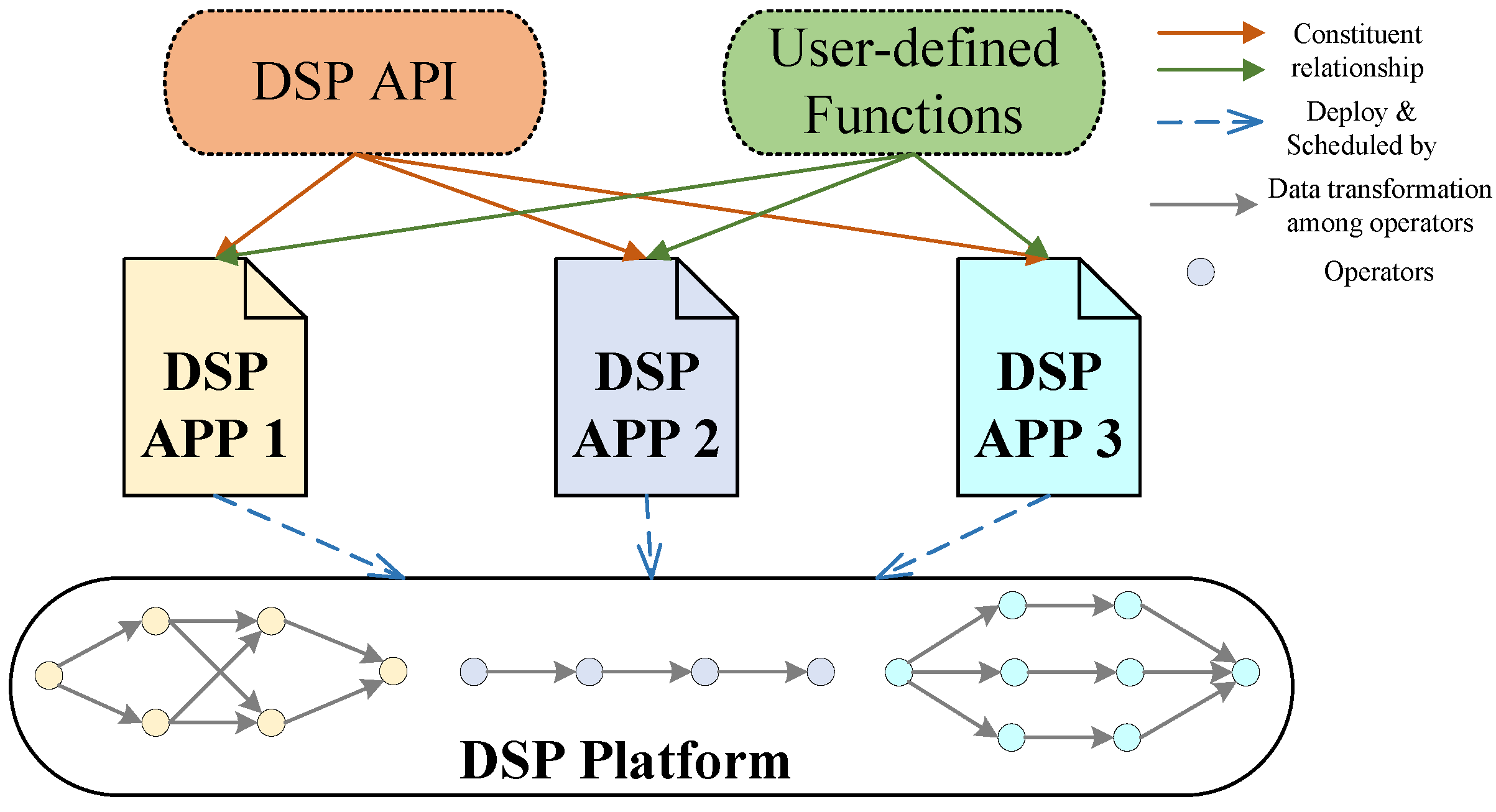
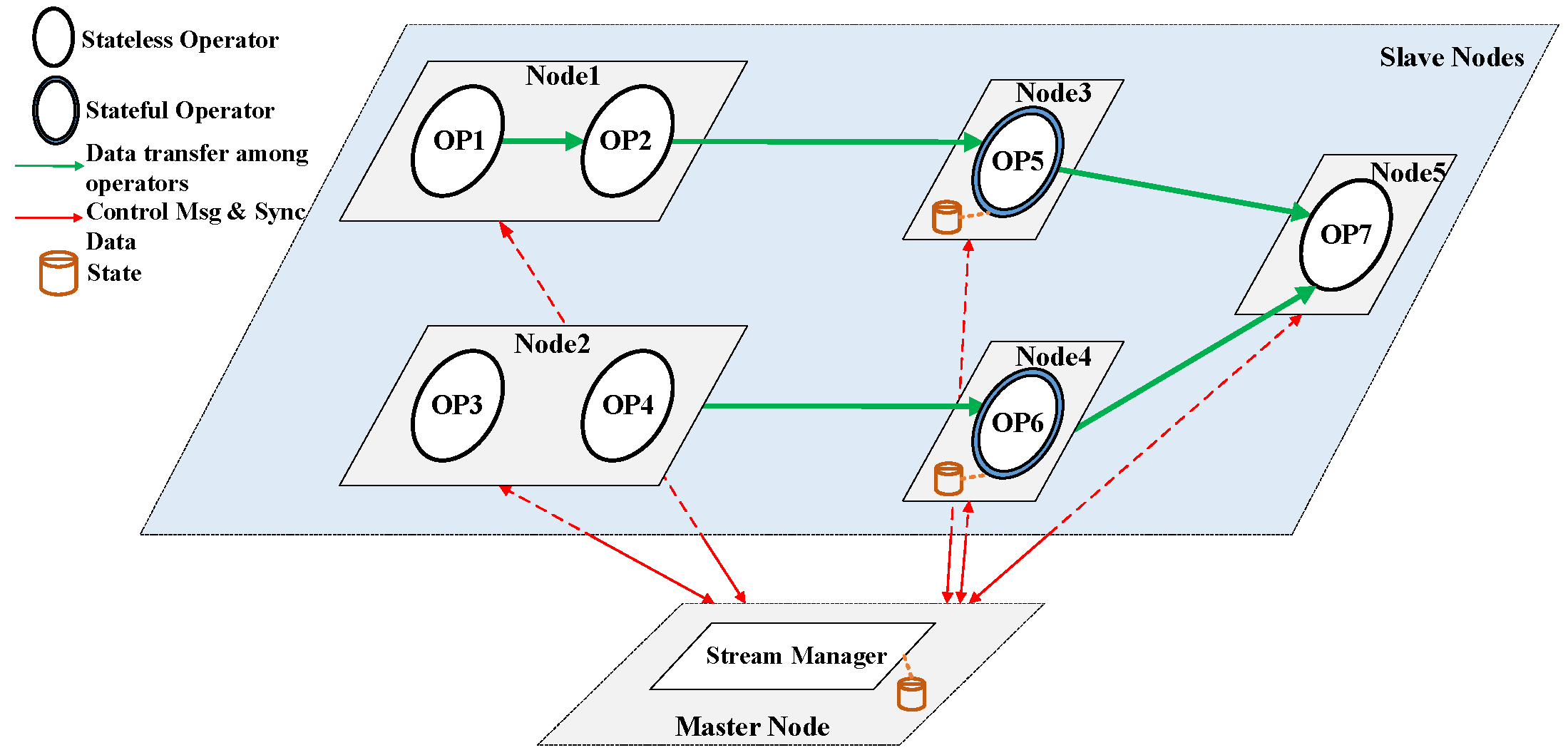
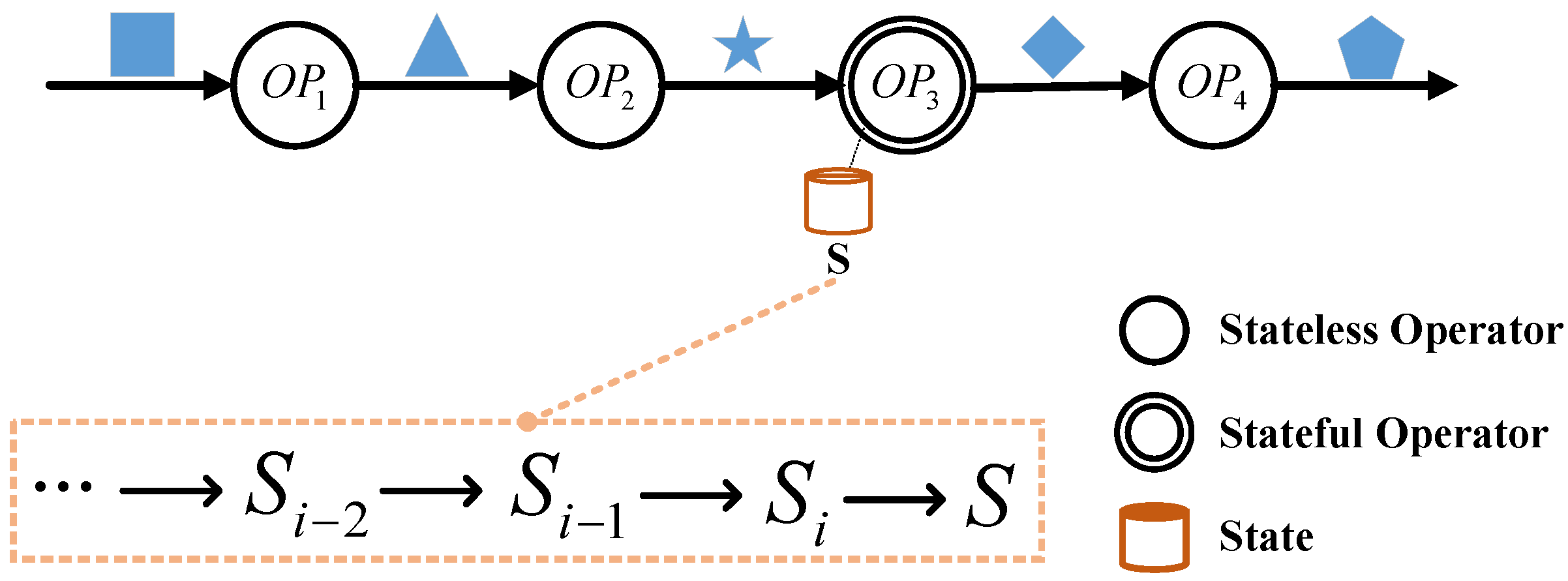
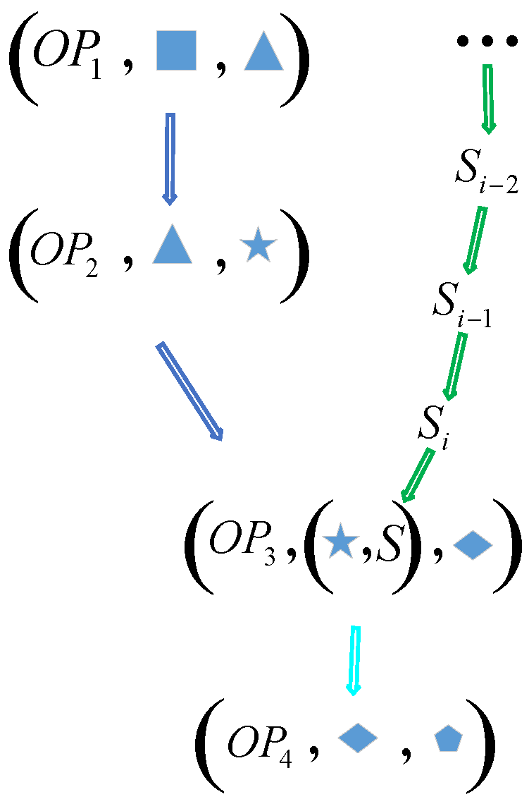
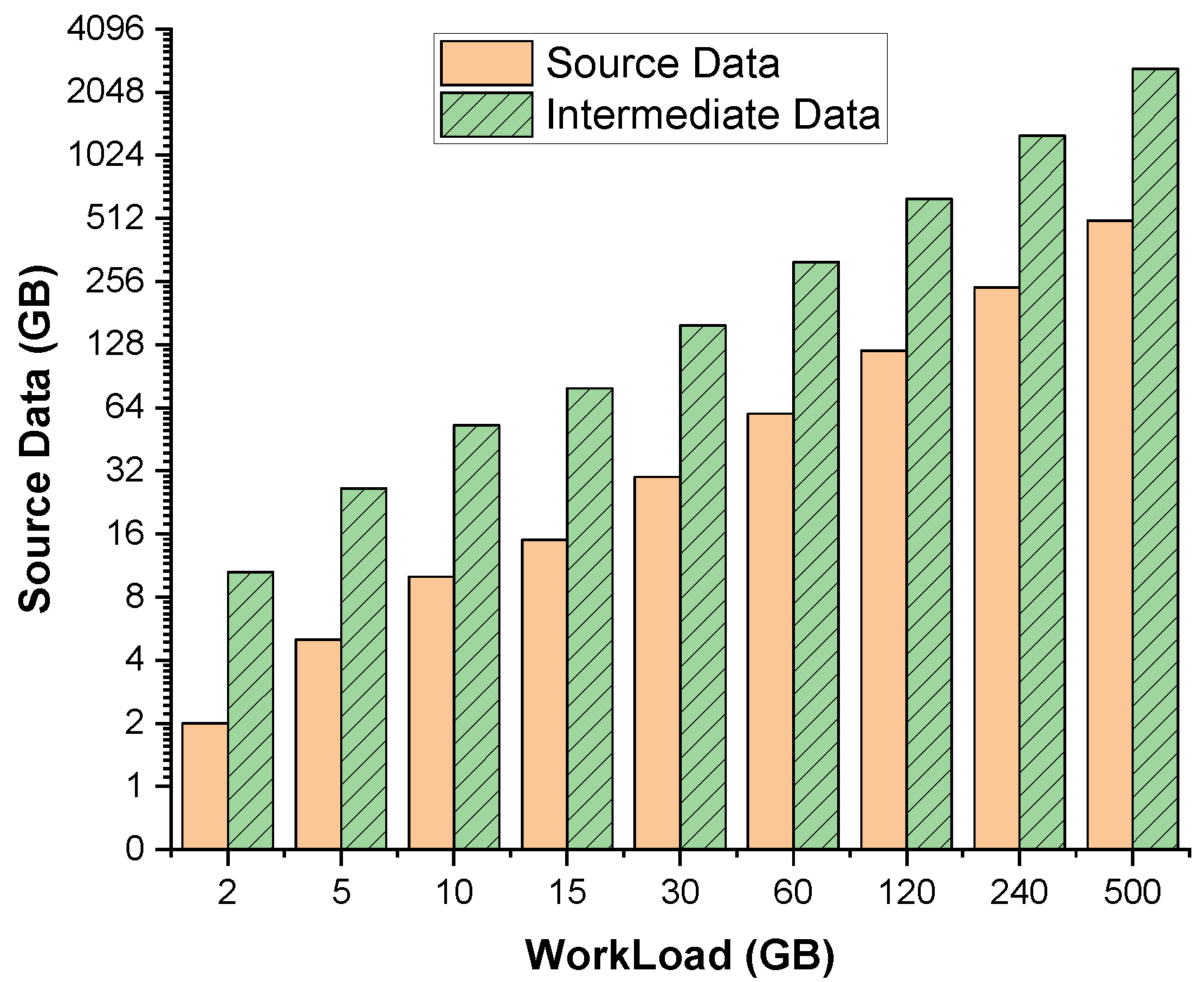
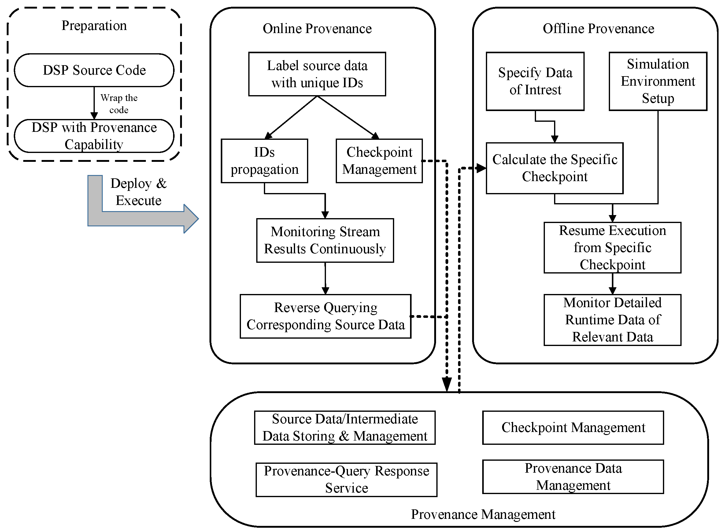
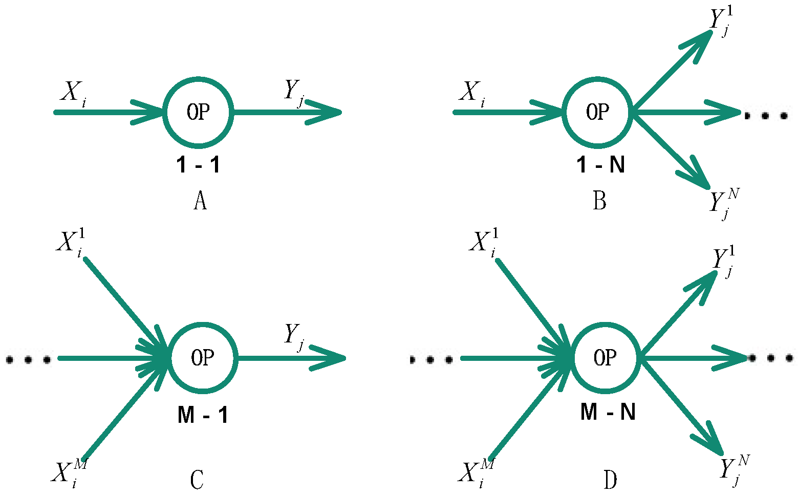
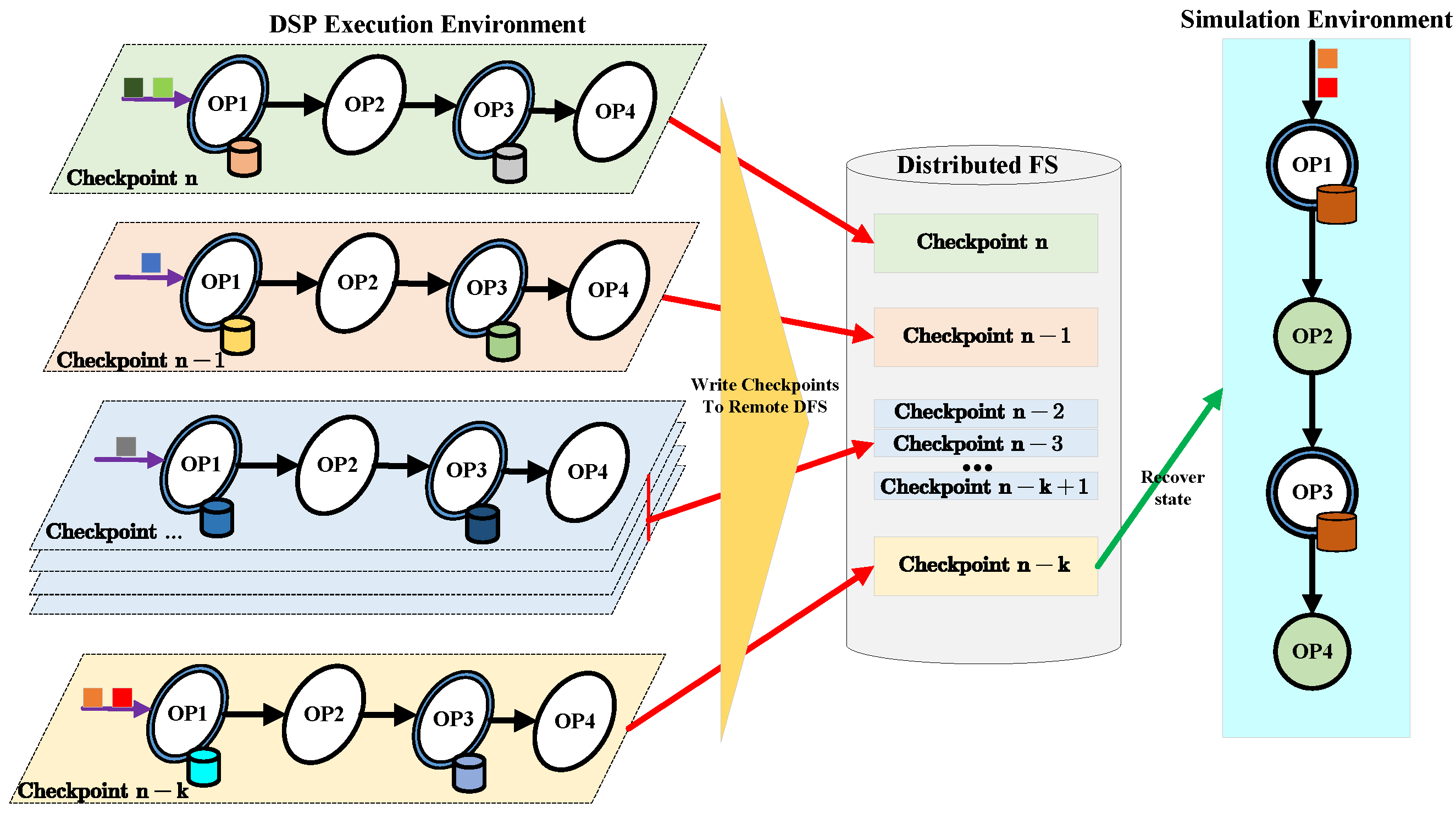
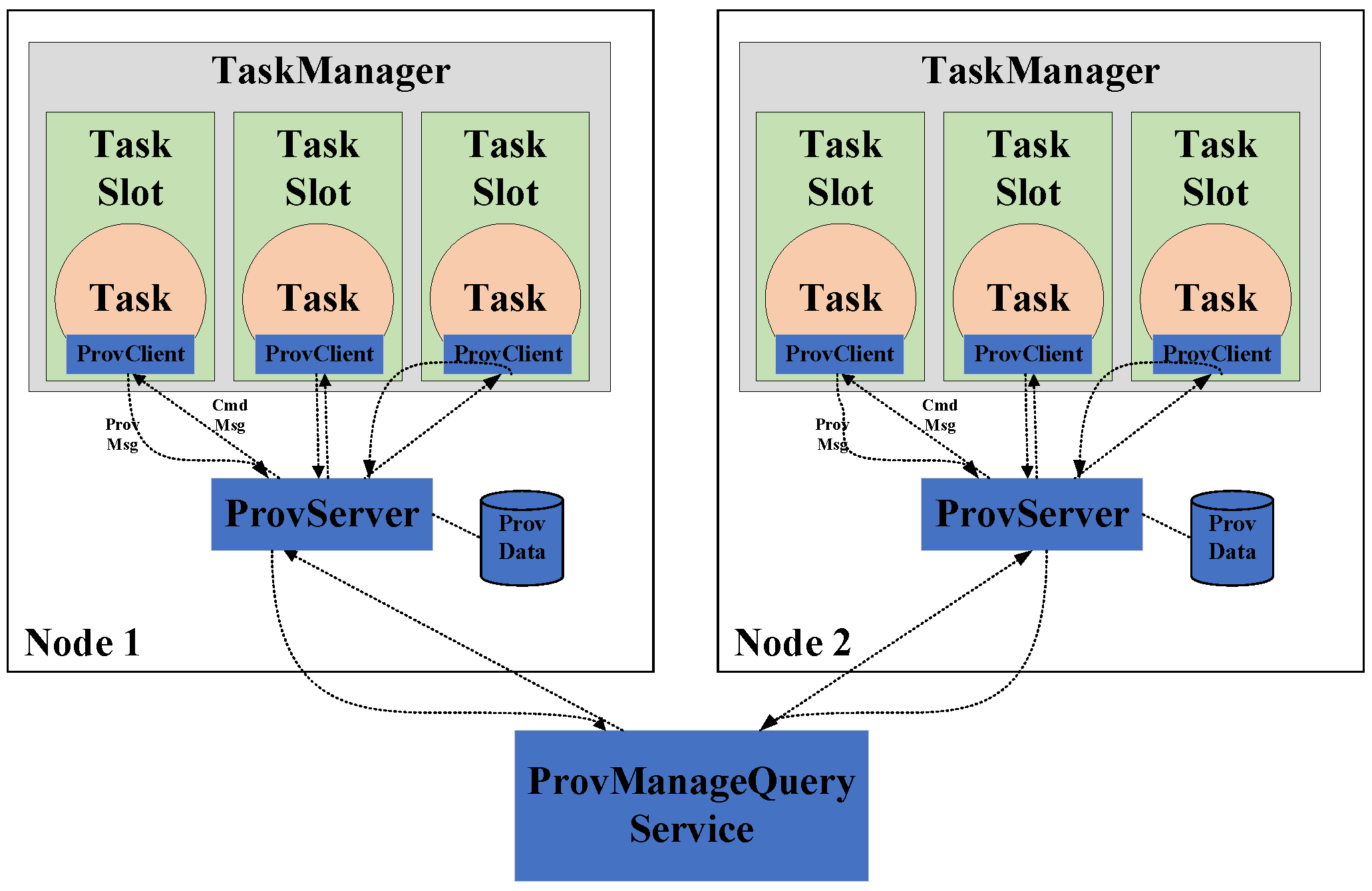
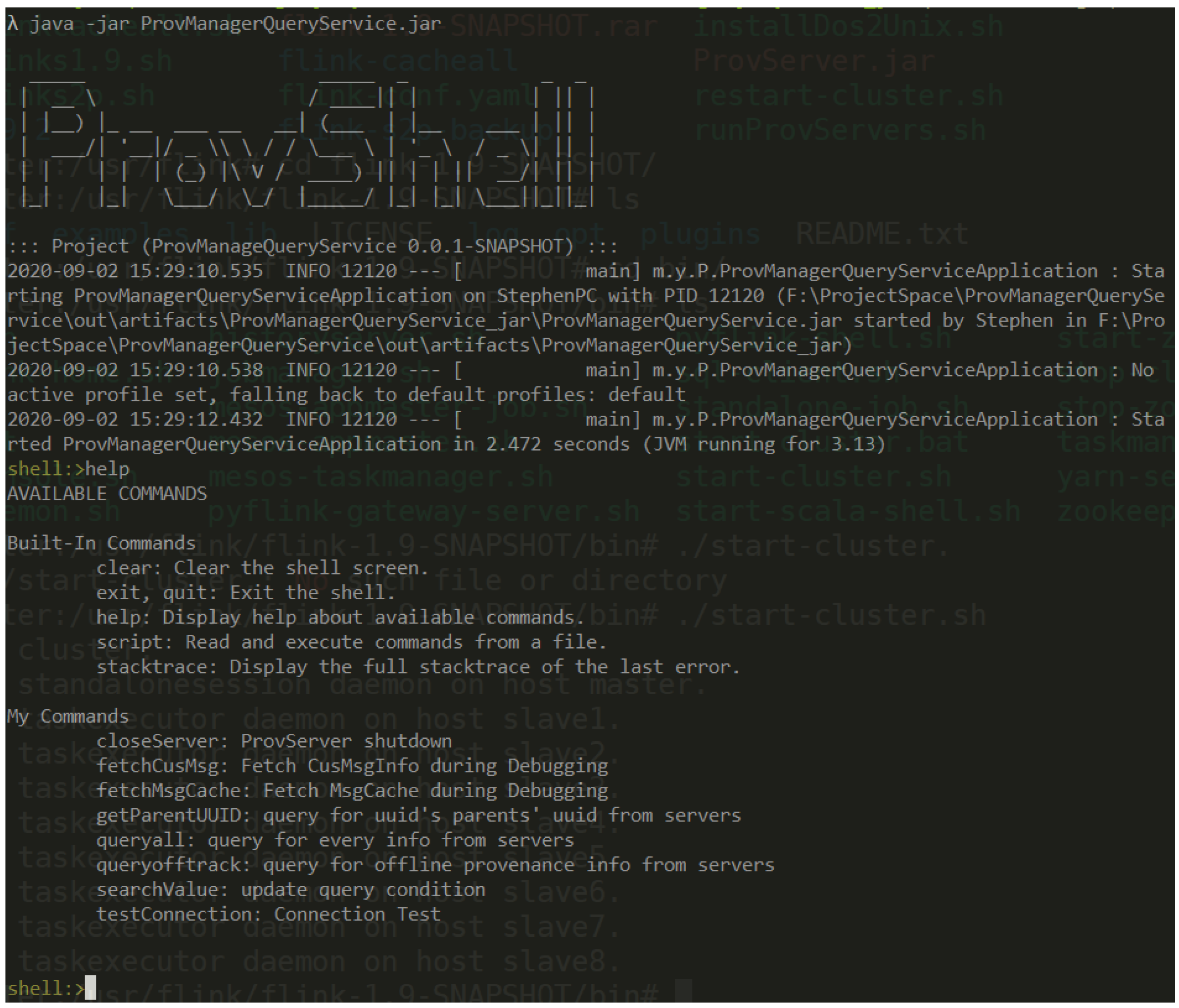
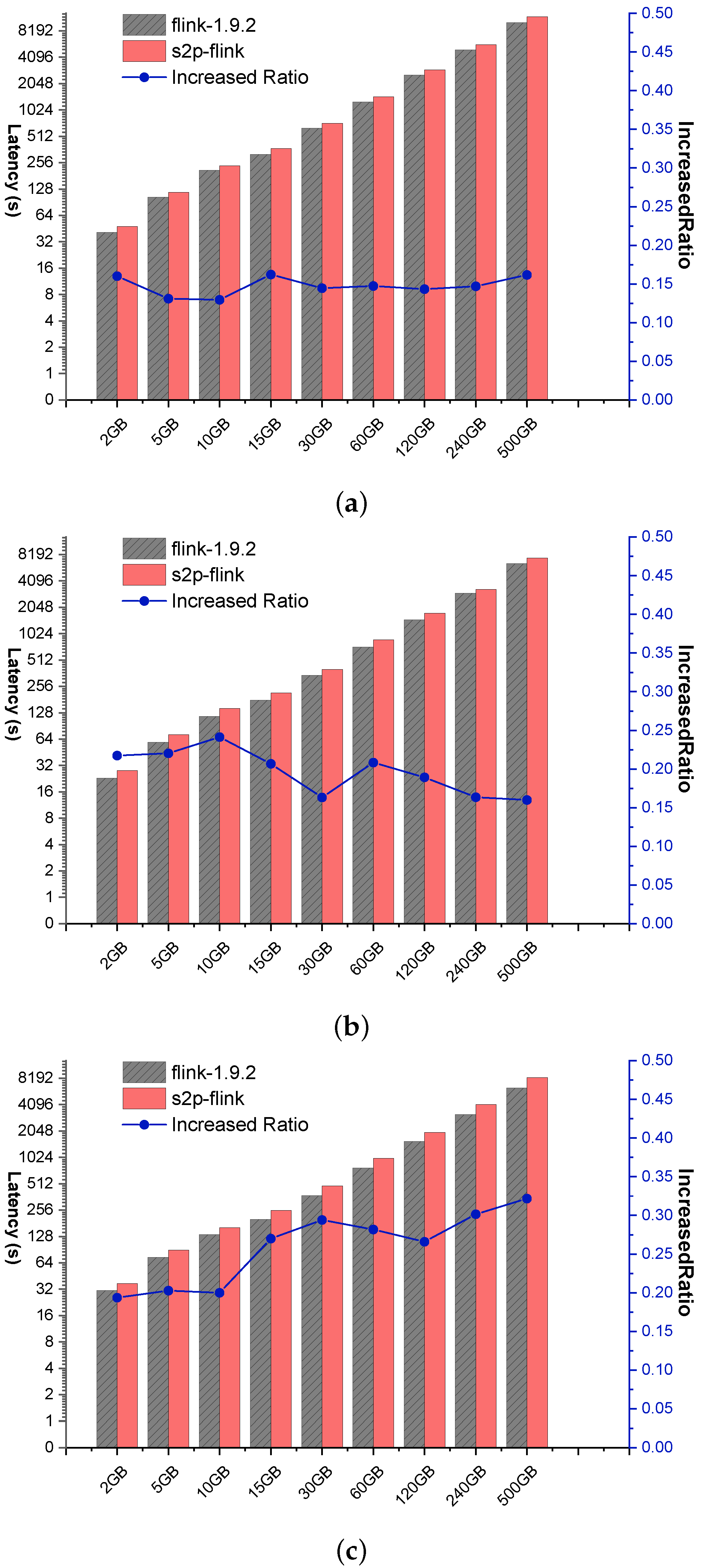
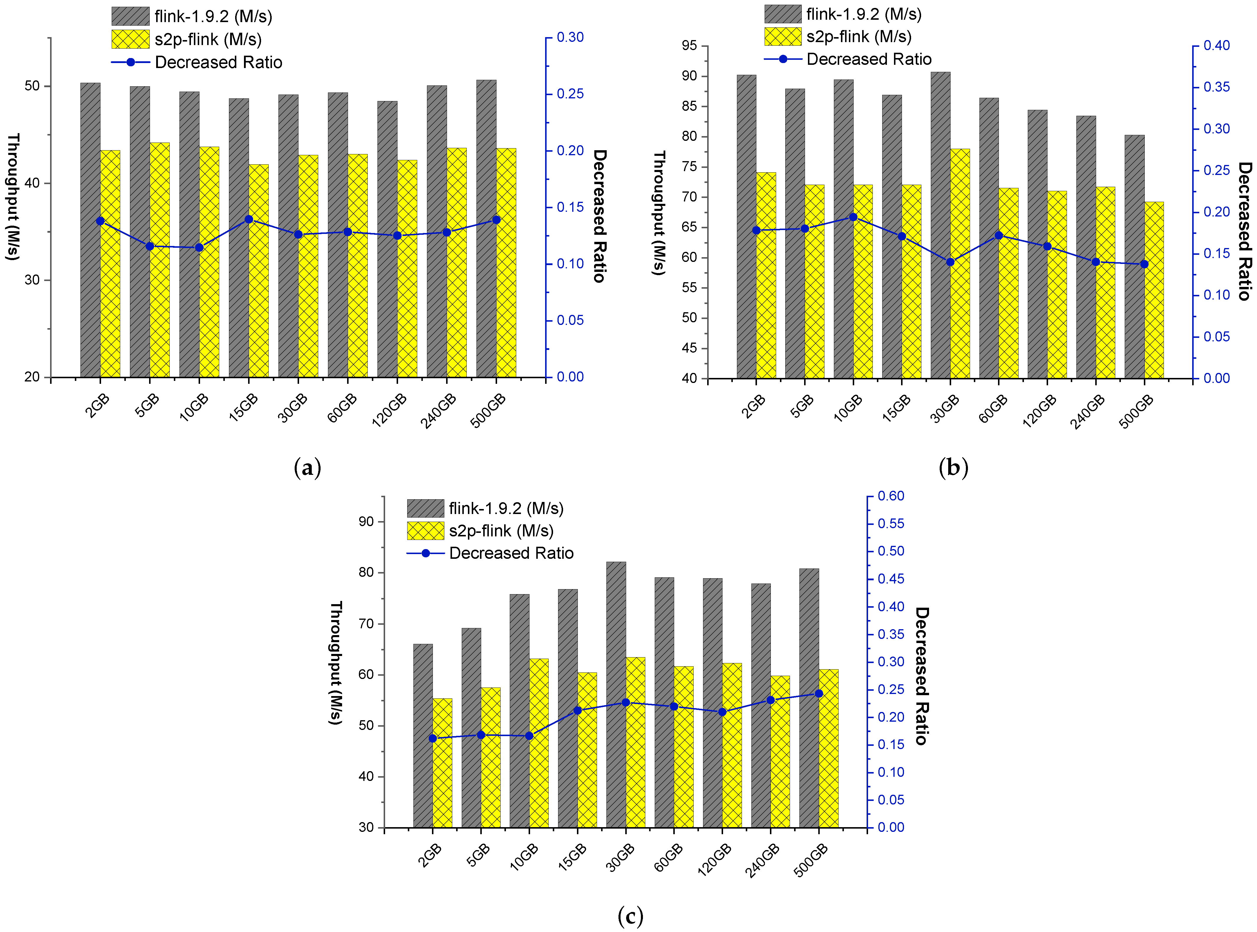
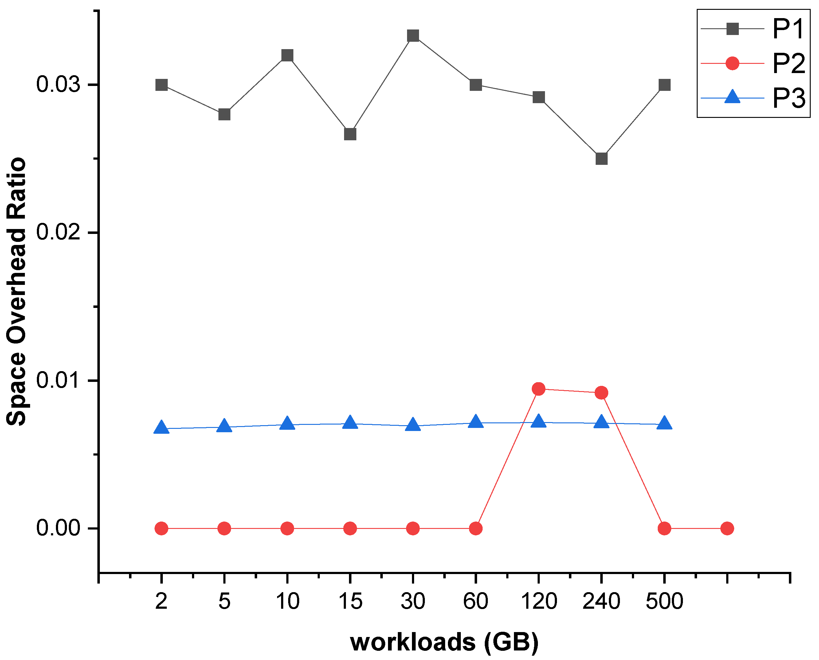
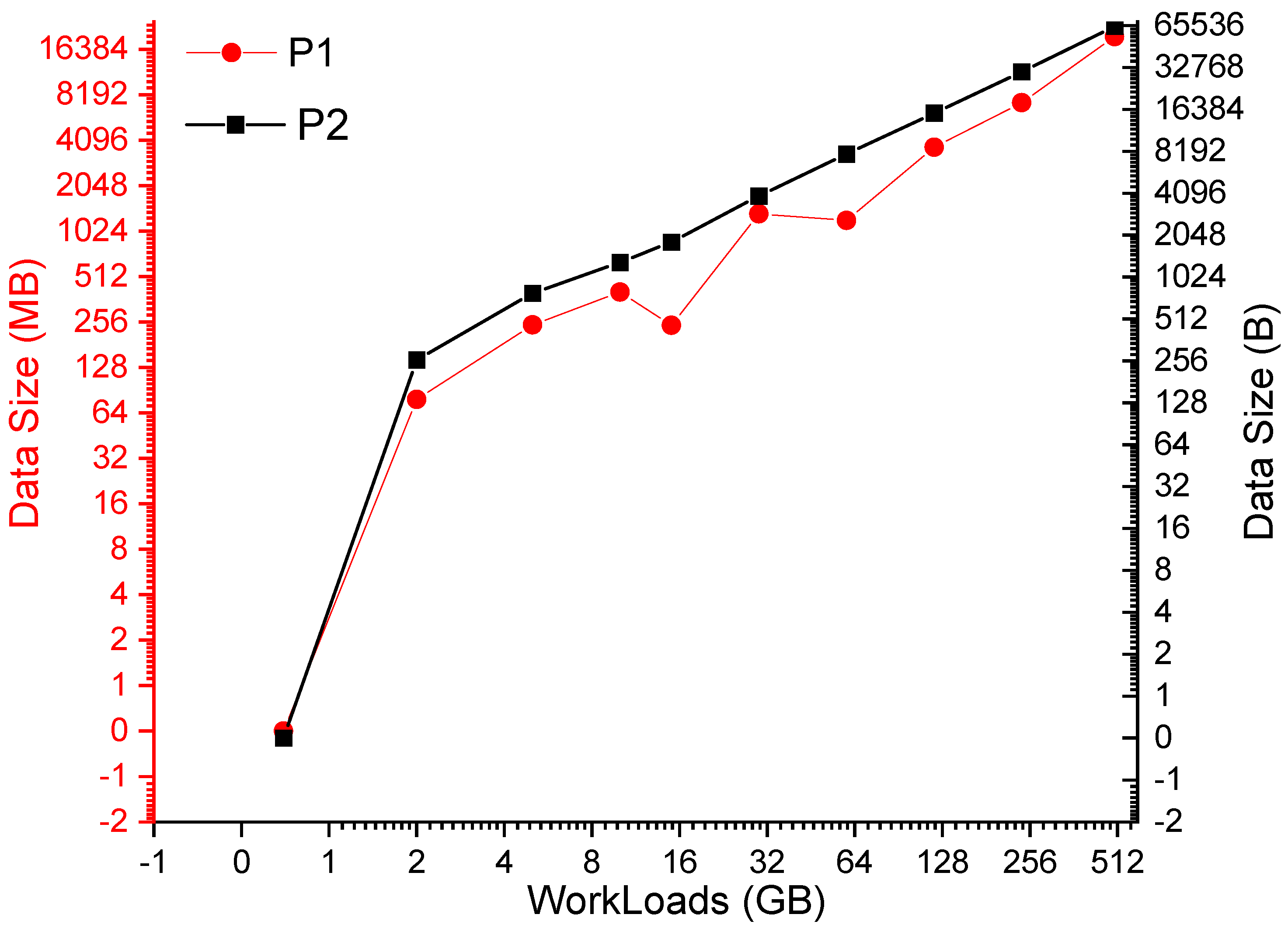
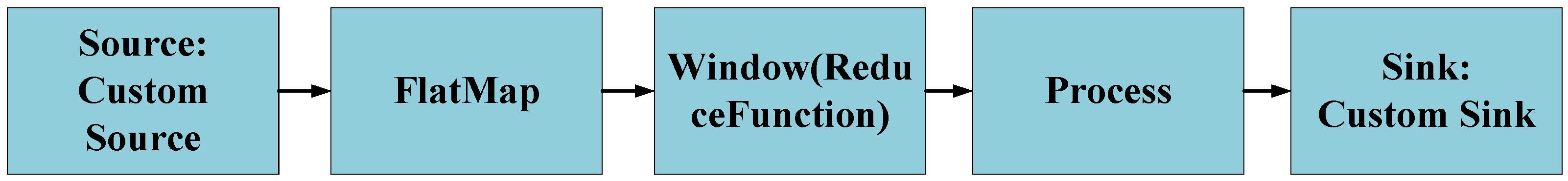
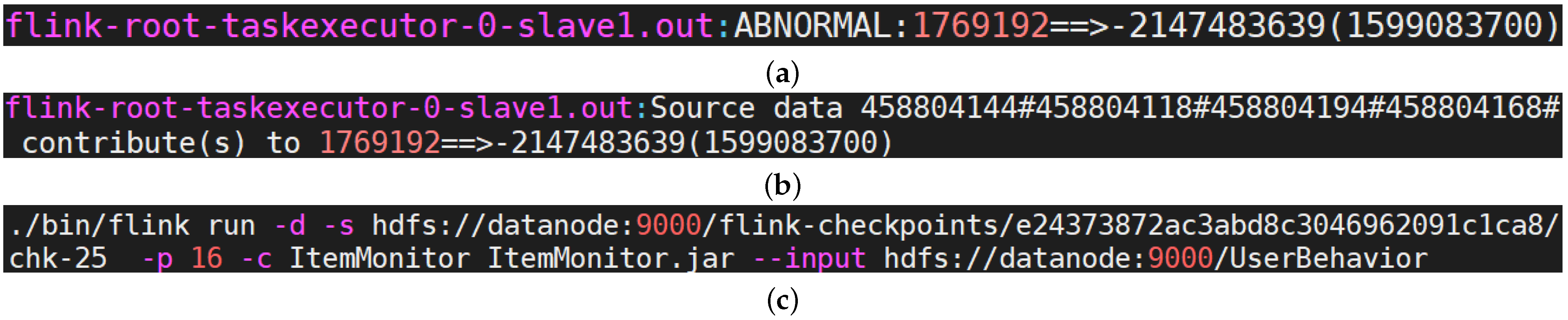
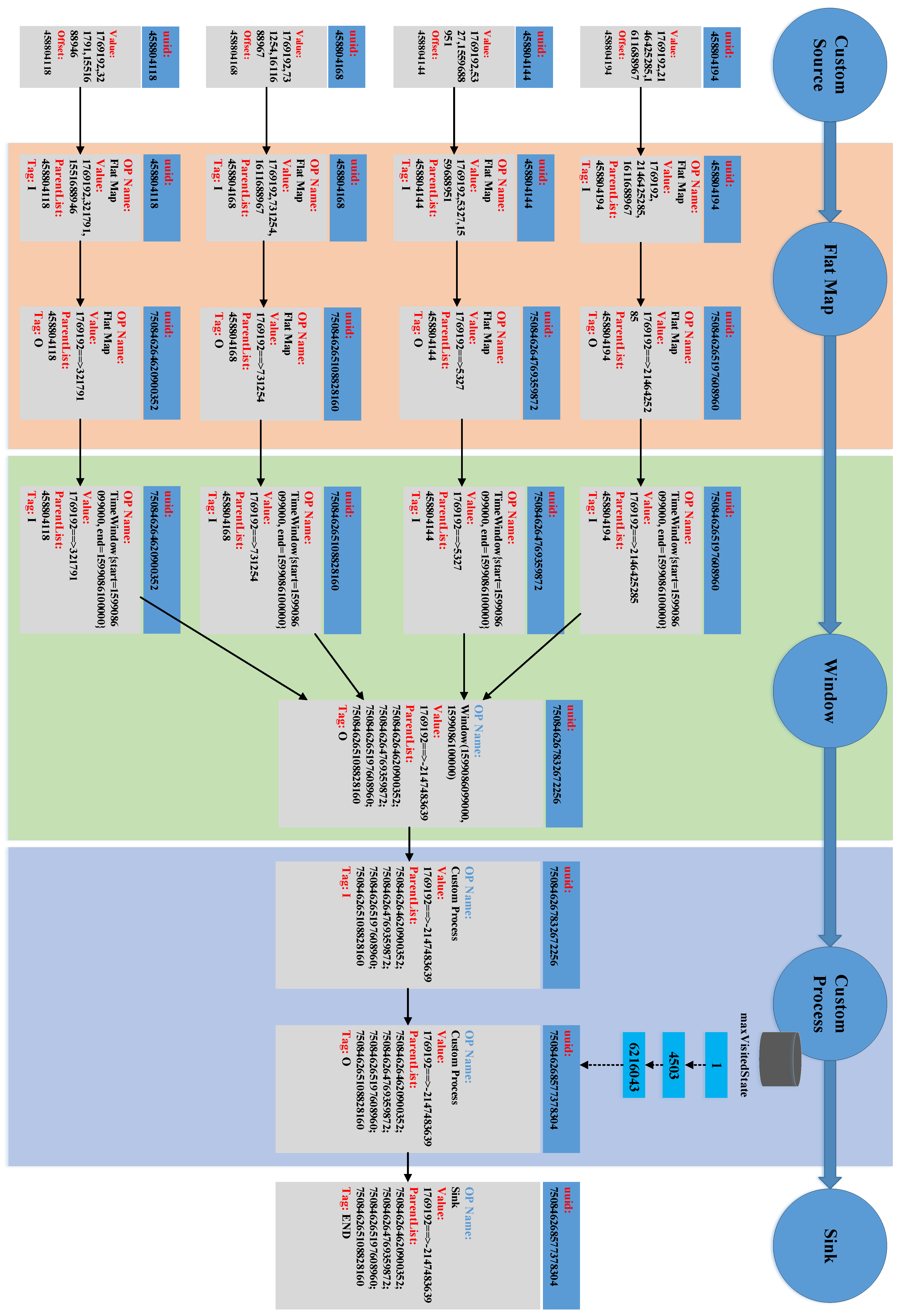
Table 1.
Summary of features in general-purpose data processing systems with provenance support.
| Provenance Systems | Provenance Support for | Provenance Storage | Provenance Tracking Granularity | Modifying Application Required (Y/N) | Intermediate Data Tracking (Y/N) | Third-Party Systems Involved (Y/N) | |
|---|---|---|---|---|---|---|---|
| >Batch-processing Oriented Provenance | RAMP [17] | Hadoop | HDFS | Map/Reduce Level | N | N | N |
| Newt [29] | Hadoop/Hyracks | MySQL | Multiple Levels | Y | N | Y | |
| HadoopProv [18] | Hadoop | File | Map/Reduce Level | N | N | N | |
| Lipstick [30] | Pig(Hadoop) | File | Operator Level | Y | N | N | |
| Titian [19] | Spark | Native | Spark Stage Level | N | Y | N | |
| Arthur [31] | Hadoop /Spark /Hyracks /Dryad | File | Operator Level | Y | Y | N | |
| Stream-processing Oriented Provenance | Tracing Framework [32,33] | Spark | External | Operator Level | N | Y | Y |
| Ariadne [22,23] | Borealis | File | Operator Level | Y | Y | N | |
| GeneaLog [4,24] | Flink /Liebre | Memory | Operator Level | Y | N | N | |
| On-the-fly provenance tracking [34] | Not specific | External | Operator Level | Y | N | Y |
They sampled the data. Strictly speaking, their solution can track partial intermediate data.
Table 2.
Subject Applications.
| # | Subject Application | Output | # Of Operators | Operators | Input Sizes |
|---|---|---|---|---|---|
| P1 | WordCount | Counts the times each word appears at regular intervals | 4 | FlatMap, KeyBy, Window, Reduce | 2G, 5G, 10G, 15G, 30G, 60G, 120G, 240G, 500G |
| P2 | Grep | Finds the words in the input data sets that match any one in one given list of words | 2 | FlatMap, Filter | |
| P3 | MovieRatings | Finds movies with scores greater than four | 7 | Map, Filter, KeyBy, Window, Reduce |
Table 3.
Latency comparison results for P1, P2, and P3 applications under various workloads on s2p-flink and native Flink.
Table 3.
Latency comparison results for P1, P2, and P3 applications under various workloads on s2p-flink and native Flink.
| WorkLoads | P1 | P2 | P3 |
|---|---|---|---|
| 2 GB | 1.16X | 1.22X | 1.19X |
| 5 GB | 1.13X | 1.22X | 1.20X |
| 10 GB | 1.13X | 1.24X | 1.20X |
| 15 GB | 1.16X | 1.20X | 1.27X |
| 30 GB | 1.14X | 1.16X | 1.29X |
| 60 GB | 1.15X | 1.21X | 1.28X |
| 120 GB | 1.14X | 1.19X | 1.26X |
| 240 GB | 1.15X | 1.16X | 1.30X |
| 500 GB | 1.16X | 1.16X | 1.32X |
Table 4.
Statistical results for increased cost ratio of P1, P2, and P3.
| P1 | P2 | P3 | |
|---|---|---|---|
| Mean | 0.146 | 0.196 | 0.257 |
| Median | 0.15 | 0.2 | 0.27 |
| Variance () | 0.0001 | 0.0008 | 0.0021 |
Table 5.
Source IDs with their corresponding source data and the latest checkpoint before the source data are ingested.
Table 5.
Source IDs with their corresponding source data and the latest checkpoint before the source data are ingested.
| Source Data’s ID | Source Data | Checkp. |
|---|---|---|
| 458804144 | 1769192,5327,1559688951 | chk-25 |
| 458804118 | 1769192,321791,1551688946 | chk-25 |
| 458804194 | 1769192,2146425285,1561688967 | chk-25 |
| 458804168 | 1769192,731254,1573688967 | chk-25 |
Table 6.
Optimization solutions to reduce runtime overhead for big data provenance.
| Optimization Strategies | Provenance Systems | Target |
|---|---|---|
| Source data sampling | Tracing Framework [32,33] | Processing Time |
| Fixed-size provenance annotation | GeneaLog [4,24] | Latency/Throughput |
| Intermediate data reduction | Newt [29] | Processing Time |
| Titian [19] | Processing Time | |
| Arthur [31] | Processing Time | |
| On-the-fly provenance tracking [34] | Throughput | |
| Generate provenance lazily | Ariadne [22,23] | Processing Time |
Publisher’s Note: MDPI stays neutral with regard to jurisdictional claims in published maps and institutional affiliations. |
© 2021 by the authors. Licensee MDPI, Basel, Switzerland. This article is an open access article distributed under the terms and conditions of the Creative Commons Attribution (CC BY) license (https://creativecommons.org/licenses/by/4.0/).
Share and Cite
MDPI and ACS Style
Ye, Q.; Lu, M. s2p: Provenance Research for Stream Processing System. Appl. Sci. 2021, 11, 5523. https://doi.org/10.3390/app11125523
AMA Style
Ye Q, Lu M. s2p: Provenance Research for Stream Processing System. Applied Sciences. 2021; 11(12):5523. https://doi.org/10.3390/app11125523
Chicago/Turabian StyleYe, Qian, and Minyan Lu. 2021. "s2p: Provenance Research for Stream Processing System" Applied Sciences 11, no. 12: 5523. https://doi.org/10.3390/app11125523
Note that from the first issue of 2016, this journal uses article numbers instead of page numbers. See further details here.