Visual Analysis of Spatiotemporal Data Predictions with Deep Learning Models

Abstract

The output of a deep-learning model delivers different predictions depending on the input of the deep learning model. In particular, the input characteristics might affect the output of a deep learning model. When predicting data that are measured with sensors in multiple locations, it is necessary to train a deep learning model with spatiotemporal characteristics of the data. Additionally, since not all of the data measured together result in increasing the accuracy of the deep learning model, we need to utilize the correlation characteristics between the data features. However, it is difficult to interpret the deep learning output, depending on the input characteristics. Therefore, it is necessary to analyze how the input characteristics affect prediction results to interpret deep learning models. In this paper, we propose a visualization system to analyze deep learning models with air pollution data. The proposed system visualizes the predictions according to the input characteristics. The input characteristics include space-time and data features, and we apply temporal prediction networks, including gated recurrent units (GRU), long short term memory (LSTM), and spatiotemporal prediction networks (convolutional LSTM) as deep learning models. We interpret the output according to the characteristics of input to show the effectiveness of the system.

1. Introduction

Spatiotemporal data contain feature information, such as temporal and spatial information, at the same time [1]. Therefore, spatiotemporal correlation patterns are often utilized together in prediction models. Spatiotemporal prediction models are applied in various fields, such as traffic, weather, social media, flights, and human migration. However, creating a prediction model is challenging because each field has a different degree and type of spatiotemporal correlation and complexity [2]. Different means of recording spatiotemporal data and different data formats make predictions more complicated. Radar echo data and air pollutant data have different recording schemes and data formats. Radar echo data are signals reflected from objects, such as raindrops. Radar echo data sets can be collected in the form of a two-dimensional image sequence in a regular grid. On the other hand, air pollutant data are recorded with air-condition information from sensors. Most air pollutant data are continuously recorded in time but have uneven spatial information, due to irregular sensor locations, which is more complicated for spatiotemporal pattern extraction.

In machine learning [3], the machine is trained using data and algorithms to learn how to perform a task. Deep learning [4] is considered an evolution of machine learning, which uses a programmable neural network that empowers the machine to make decisions without guidance from humans. There are two methods in machine learning, including supervised learning and unsupervised learning. The main difference between these two is the use of labeled data sets. Supervised learning utilizes labeled input and output data, while unsupervised learning does not. Deep learning models can be applied for temporal pattern prediction. Typically, recurrent neural networks (RNNs) use recurrent computations to train temporal patterns from historical sequence information and produce predictions. Many studies were conducted to predict spatiotemporal data with gated recurrent unit (GRU) networks and long short term memory (LSTM) networks with RNN structures [5,6,7], which have a looping constraint on the hidden layer of the artificial neural network (ANN). Preprocessing is expected to handle spatiotemporal data as input to the RNN architectures. Since the RNNs do not consider the spatial structure, the spatial information within the data may be dropped during the preprocessing.

A spatiotemporal predictive deep-learning model was proposed to resolve the problem in RNN that does not consider the spatial structure. The convolutional LSTM network [8] recognizes the spatiotemporal correlation by combining the LSTM layer and the convolutional layer. Although this deep learning model predicts spatiotemporal data adequately, it is puzzling to understand how the incorporation of spatial information in the input data can improve the predictive performance of the deep learning model, just by reviewing the accuracy. Since the spatial information contained in each feature of the data is different, the prediction performance also varies, according to the feature selection. In addition to the feature selection, the incorporation of spatial information, such as grid structure, also affects the deep learning performance. Therefore, it is challenging to interpret deep learning results that depend on input characteristics such as feature selection, temporal correlation, and spatial correlation. The more difficult the deep learning model is to interpret, the more time-consuming the modeling process is. Hence, it is necessary to develop a system that allows us to quickly interpret the output of the deep learning model, according to the input characteristics. The contributions of our work are as follows.

• We develop a visualization system to support the interpretation of outputs from deep learning models.
• We propose multiple feature selection functionalities with temporal and spatial information.
• Our system enables us to perform prediction modelings by visualizing information, such as correlations between variables, temporal autocorrelation, and spatial autocorrelation.
• We evaluate our system through prediction modeling for a spatiotemporal air pollutant data set.

We expect that our system supports us in understanding deep learning modeling and exploring the results with data and parameters interactively for prediction improvements.

2. Related Work

Many researchers desire to understand how deep learning models are trained, how model representations are interpreted, and how deep learning supports decision making [9]. The idea of model understanding in machine learning is divided into interpretability and explainability [10]. The interpretation is to understand the status transitions that occur while changing input or algorithm parameters in machine learning models. Explainability is the interpretation of the internal mechanisms of machine learning models in understandable human terms.

In visualization and visual analytics (VA) areas, some studies have been proposed to support the design and debugging of models by applying VA to an interactive machine learning workflow [9]. In the area of model interpretation, visual analytics has focused on understanding the structure of models [11], analyzing the performance of predictive models [12], identifying misclassified instances [13,14,15], and comparing the performance of multiple predictive models [16]. To explain the structure of the model, node-link diagrams [17], drawing directed graphs [11], and directed acyclic graphs [18] are applied. Wongsuphasawat et al. [11] presented a TensorFlow graph visualizer to assist in understanding machine learning architectures. Liu et al. [18] proposed a visual analytics system to understand and diagnose a convolutional neural network, using a directed acyclic graph. Although many visual analysis systems support machine learning modeling, most are limited in classification models. Therefore, we believe that our system assists us in understanding deep learning modeling while improving spatiotemporal predictions.

The performance analysis of the predictive model includes studies to explore the combination of input features [19] and to improve the quality of the labeled data [13,20]. Xiang et al. [13] introduce a system for correcting false labels in training data, using hierarchical visualization with incremental t-distributed stochastic neighbor embedding (t-SNE). If we can observe the cause and consequence of the predictive model in interactive machine learning, the explainable AI (XAI) must be able to analyze why the model makes such a decision [21]. To understand the internal mechanism, researchers detect errors or weight changes observed in specific output changes during the learning process based on the performance metrics [22]. Comprehensive theoretical studies of the role of visual analytics in deep learning have been conducted, and it is possible to interpret various deep learning models, such as CNN [23], DNN [24], RNN [25,26], LSTM [27,28], and DQN [29]. Spinner et al. [22] also presented an interactive and explainable visual analytics framework for understanding machine learning models. They can diagnose and improve the limitations of the designed model through quality monitoring, provenance tracking, and model comparison in the TensorBoard environment.

In the field of statistics, time-series data predictions are mainly performed with the autoregressive model, moving average model, and autoregressive moving average (ARIMA) model. In machine learning studies, the RNN and LSTM are known to be suitable for time series prediction. LSTM models can be constructed according to the layer layout, structure, connectivity, and combination with other neural networks. Typical LSTM models are Vanilla LSTM [30], Stacked LSTM [31], Bidirectional LSTM [32], etc. Although the LSTM model generally outperforms the ARIMA model in time series prediction [33], the ARIMA model outperforms the LSTM in time series data with strong seasonal factors [34]. Studies for the interpretation of LSTMs and RNNs were published in the visual analytics community. Tang et al. [35] visualized the behavior of LSTM and GRU in speech recognition and presented that LSTM has long-term memory but is more sensitive to noise than RNN. Strobelt et al. [36] provided a visual tool to improve the performance of LSTM models with the exploration and summarization of long-term dependencies in time series and sequence data. Since our data have temporal features, we employ LSTM and GRU for deep learning modeling.

Spatial interpolation estimates the unobserved data inside the sampled area with the observed data [37]. Spatial interpolation is generally applied for visualization, mainly by computing the pixel values from pixel-based data [38]. Many algorithms were developed for interpolation, including nearest-neighbor interpolation, bilinear interpolation, and bicubic interpolation [39]. Inverse distance weighted interpolation (IDW) is assumed to have similar values as the data become closer to each other [40]. IDW interpolation estimates the value of an unknown point by weighting it inversely with distance [41]. IDW interpolation assigns consecutive weights, while nearest-neighbor interpolation weights only 1 to the nearest data. Linear interpolation is a simple interpolation that estimates data linearly. We can use cubic interpolation to reduce the discontinuities caused by linear interpolation. Cubic interpolation produces more smooth data than linear interpolation or nearest-neighbor interpolation. As a high-order interpolation, radial basis function (RBF) is employed for more accurate interpolation of unstructured data. The RBF interpolation can be constructed in an artificial neural network by using RBFs as activation functions [42]. In this work, we apply cubic, linear RBF, and nearest-neighbor techniques for spatial interpolation.

Prediction of spatiotemporal data is generally performed considering both the temporal and spatial feature points. Deep learning algorithms that are mainly used for space-time data prediction include LCRN [43] and convolutional LSTM (ConvLSTM) [8]. LCRN has a structure in which CNN and LSTM are sequentially connected. In the LCRN structure, the spatiotemporal data inputs are trained for the spatial feature points with the CNN and the temporal feature points with the LSTM. Johan et al. [44] presented PVNet, using the LCRN structure. PVNet predicts photovoltaic power by training numerical weather information, including irradiance, cloud, temperature, the clear sky model and a power model, calculated with the persistence model. LCRN contains a sequential connection structure between CNN and LSTM, while ConvLSTM includes convolution operations within the cells of LSTM. ConvLSTM trains spatiotemporal data by performing convolution operations as soon as input data are inserted into LSTM cells. ConvLSTM has faster computational speed and has higher performance than LCRN in many studies. Yuan et al. [45] conducted a study on the traffic accident prediction problem, using the ConvLSTM model. They predicted data by applying a spatial ensemble to the results predicted by ConvLSTM. The proposed model shows a much higher prediction accuracy than the conventional method. He et al. [46] proposed STCNN using ConvLSTM for long-term traffic predictions. The proposed model combines the weekly ConvLSTM prediction result and the daily Skip-ConvLSTM prediction result for CNN training to identify the periodic pattern of traffic. Lin et al. [47] proposed a ConvLSTM-based spatiotemporal temperature deviation prediction model (PredTemp). They compared the predictions with ConvLSTM, using temperature deviation data, and with ConvLSTM, using both precipitation and temperature deviation data. To utilize spatiotemporal features, we also include ConvLSTM for deep learning modeling.

3. Data Description

Particulate matter (PM) is a particle that is generated naturally or artificially and is contained in the air as an aerosol. The most commonly used PM parameters include ${\mathrm{PM}}_{10}$, whose diameter is 10 micrometers or less, and ${\mathrm{PM}}_{2.5}$, whose diameter is 2.5 micrometers or less. PM is a fine particle that floats in the air and is a respirable substance that has a significant impact on health. Many countries around the world treat PM as an environmental issue. In October 2013, the World Health Organization (WHO) and the International Agency for Research on Cancer (IARC) classified PM as a Class 1 carcinogen, due to the high toxicity. According to the State of Global Air [48] released in 2018, 33.7% of the world was exposed to household air pollution in 2016, and the death toll associated with ${\mathrm{PM}}_{2.5}$ reached 4.1 million by 2016.

PM tends to float in the air and propagate with the flow of the atmosphere. The smaller the PMs, the longer they stay in the air. The diffusion rate varies depending on the particle compositions. The PM forecast is a challenge for climate forecasts, as they show different patterns depending on the climate impact of each country. PM data are the density of the particulate matter, such as ${\mathrm{PM}}_{2.5}$ and ${\mathrm{PM}}_{10}$ collected from ground stations. In general, it is desirable for the stations to be evenly distributed throughout the country but they usually tend to be concentrated in major cities and towns. The distribution is not even uniform, which makes it challenging to predict such spatiotemporal data.

In this paper, we compare the performances of deep learning models to predict air pollutant data as spatiotemporal data. We utilize air pollutant data provided by kweather [49]. Data were collected from 413 discrete stations in Seoul, South Korea. The collected data include ${\mathrm{PM}}_{2.5}$, ${\mathrm{PM}}_{10}$, noise, temperature, and humidity, and we utilize data that were measured every hour for 75 days from 5 September 2019, to 18 November 2019. We examined the missing data as preprocessing and removed 16 days of data. We also scaled all the data, using min–max scaling. To properly apply deep learning models, the models are trained with the training data, and the model parameters are tuned with the validation data. Then, the model performance is evaluated with the test data, which are unbiased. We randomly separated the data sets into 991, 212, and 213 h for the training data set, validate data set and test data set, respectively, at the ratio of 7:1.5:1.5. In this paper, we design PM prediction models using these data sets and compare the PM prediction performance depending on the data feature selection and temporal and spatial correlations with deep learning models.

4. Spatiotemporal Prediction Models

In this paper, we compare spatiotemporal data prediction models using deep learning and investigate the prediction performances according to deep learning models and training data sets. The prediction performance of spatiotemporal data varies depending on the feature selection, temporal correlation, and spatial correlation of the input data. Therefore, a comprehensive review of spatiotemporal data is essential to understand prediction performance. We examine the performance of deep learning prediction models in terms of feature selection and spatiotemporal correlation. This section presents the algorithms used to analyze how features, temporal correlations, and spatial correlations affect the predictive performance.

4.1. Feature Selection with Correlations

Feature selection is the process of constructing a subset of correlated variables and is an essential technique that is directly related to training performance. In general, feature selection generates a data subset according to the data relationships, such as mutual information and the Pearson correlation coefficient. However, the feature selection of spatiotemporal data makes it challenging to choose subsets based only on simple correlation coefficients or scores because we must examine both temporal and spatial relationships. In this work, we employ the Pearson correlation coefficient, temporal autocorrelation, spatial autocorrelation, and the LISA algorithm to support the feature selection of the spatiotemporal data.

The linearity of correlation between variables is meaningful in determining feature association. We employ the Pearson correlation coefficient, visualize the correlations, and use it as an indicator of feature selection, depending on the data features. We also visualize temporal and spatial autocorrelation of features. We visualize LISA (local indicators of spatial association) values as indicators of spatial association. In addition to the feature selection, feature extraction techniques, such as PCA, t-SNE, and LDA, can also be applied. However, this paper does not cover features from feature extraction techniques.

4.2. Deep Learning Models for Temporal Prediction

We compare temporal prediction and spatiotemporal prediction algorithms to see how the prediction performance changes with and without spatial information. Deep learning for temporal forecast is examined, focusing on RNN, and the representative algorithms are LSTM and GRU. We construct LSTM and GRU architectures as temporal prediction algorithms and convLSTM as a spatiotemporal prediction algorithm.

LSTM is a type of RNN that is a recurrent neural network designed to resolve the long-term dependencies in RNNs and to achieve faster convergence in training. Time-series training is performed by adding memory cell and a forget gate to the RNN structure. The LSTM cell is largely composed of a forget gate f, input gate i, and output gate o. The input of the LSTM cell consists of a vector $h_t$ for a short-term state state and a vector $c_t$ for a long-term state. In LSTM, the output vector $y_t$, according to the previous state $h_{t-1}$, $c_{t-1}$ and input vector $x_t$, is presented as follows [50].

$$f_t=\sigma (W_{xf}·x_t+W_{hf}·h_{t-1}+b_f)$$

(1)

$$i_t=\sigma (W_{xi}·x_t+W_{hi}·h_{t-1}+b_i)$$

(2)

$$o_t=\sigma (W_{xo}·x_t+W_{ho}·h_{t-1}+b_o)$$

(3)

$$g_t=tanh(W_{xg}·x_t+W_{hg}·h_{t-1}+b_g)$$

(4)

$$c_t=f_t⨂c_{t-1}+i_t⨂g_t$$

(5)

$$y_t,h_t=o_t⨂tanh(c_t),$$

(6)

where $W_{xf}$, $W_{xi}$, $W_{xo}$, $W_{xg}$ are weight matrices for the layers connected to the input vector $x_t$, and $W_{hf}$, $W_{hi}$, $W_{ho}$, $W_{hg}$ are weight matrices for the layers connected to the short-term state $h_{t-1}$. Additionally, $b_f$, $b_i$, $b_o$, and $b_g$ are biases for four layers. The ⨂ is an element-wise matrix multiplication. The current short-term state $h_t$ is affected by the long-term state $c_{t-1}$ and the current long-term state $c_t$ is calculated based on the long-term state $c_{t-1}$ at the previous time and the input gate $i_t$ at the present time. LSTM resolves the long-term dependence problem in RNN by transmitting the long-term state and prevents the vanishing of the gradient, using $tanh$ as a cell activation function.

The GRU algorithm utilizes only one state vector $h_t$ and controls both the forget gate and input gate with one gate controller, $z_t$. The GRU is presented as follows [51].

$$r_t=\sigma (W_{xr}·x_t+W_{hr}·h_{t-1}+b_r)$$

(7)

$$z_t=\sigma (W_{xz}·x_t+W_{hz}·h_{t-1}+b_z)$$

(8)

$$g_t=tanh(W_{xg}·x_t+W_{hg}·(r_t⨂h_{t-1})+b_g)$$

(9)

$$h_t=z_t⨂h_{t-1}+(1-z_t)⨂g_t.$$

(10)

The GRU algorithm works similar to LSTM and can perform time-series training with fewer parameters. However, since only one state is stored, it is difficult to analyze the state value of each cell. In this paper, we choose LSTM and GRU as temporal prediction algorithms and train the data to compare model performances.

4.3. Deep Learning Models for Spatiotemporal Prediction

We compare the temporal prediction algorithms with the spatiotemporal prediction algorithm to analyze how the prediction performance changes with and without spatial information. In this paper, we use convLSTM as a spatiotemporal prediction algorithm.

ConvLSTM is a network structure that can be employed to predict spatiotemporal data by applying convolution to a fully-connected LSTM structure. The LSTM cell structure itself does not change much. However, the most significant difference is that the input datum is not a vector but an image, and the convolution is added to the LSTM internal operation. The convLSTM is presented as follows [8].

$$i_t=\sigma (W_{xi}\ast x_t+W_{hi}\ast h_{t-1}+W_{ci}⨂c_{t-1}+b_i)$$

(11)

$$f_t=\sigma (W_{xf}\ast x_t+W_{hf}\ast h_{t-1}+W_{cf}⨂c_{t-1}+b_f)$$

(12)

$$o_t=\sigma (W_{xo}\ast x_t+W_{ho}\ast h_{t-1}+W_{co}⨂c_{t-1}+b_o)$$

(13)

$$g_t=tanh(W_{xg}\ast x_t+W_{hg}\ast h_{t-1}+b_g)$$

(14)

$$c_t=f_t⨂c_{t-1}+i_t⨂g_t$$

(15)

$$h_t=o_t⨂tanh(c_t),$$

(16)

where Ws are the weight matrices for the layers, and $b_f$, $b_i$, $b_o$, $b_g$ are the biases of the layers. The ⨂ is element-wise matrix multiplication, and ∗ represents a convolution operation. The input datum is convoluted in image form. In this model, the spatial information is incorporated in the convolution operation, and the recurrent structure of the LSTM incorporates the temporal information.

4.4. Spatial Interpolation Techniques

We use spatiotemporal data measured from discrete stations in our deep learning prediction models. Therefore, the prediction result of the spatiotemporal data must be visualized by interpolating discrete data in two-dimensional space. We apply the nearest, linear, and cubic interpolation to spatially interpolate and compare the predictions of the deep learning models as postprocessing. The nearest interpolation is the most basic interpolation technique, and the algorithm fills the empty space by copying the adjacent value. The linear and cubic interpolation can be applied as a higher-order interpolation technique, and these techniques usually produce excellent approximations for regularly distributed stations.

5. System Evaluation with Air Pollutant Prediction Models

In this section, we describe the deep learning modeling process within the proposed system, using spatiotemporal air pollutant data. The deep learning modeling process involves selecting features, time lags, and deep learning algorithms, according to the correlation information between variables, temporal autocorrelation, and spatial autocorrelation. The spatial autocorrelation is computed with Moran’s I [52] and the local indicator of spatial association (LISA [53]. Moran’s I is one of the representative statistics for testing global spatial autocorrelation, confirming whether the values of specific variables in the analysis target region are correlated. Moran’s I indicates how similarly the values of the variables measured in adjacent spaces are distributed. When the value of Moran’s I is close to 1, the adjacent neighboring spatial units have similar values, and when the value of Moran’s I is close to −1, the neighboring spatial units have different values. LISA (local indicator of spatial association) is sometimes called local Moran’s I because it shows local spatial dependence. LISA makes it possible to identify the occurrence of local clustering patterns of a given variable in space. The proposed visualization system supports the deep learning modeling of spatiotemporal data by visualizing the information and prediction results required for better modeling. Therefore, the system enables us to observe the prediction results of the deep learning model to discover problems within the modeling.

The purpose of deep learning modeling with the air pollutant data introduced in Section 3 is to predict the amount of air pollution in the future. In this paper, we train ${\mathrm{PM}}_{2.5}$ with the temporal and spatiotemporal predictions of deep learning models. Then, we calculate the mean absolute percentage error (MAPE) from the test data set not used for the training as a measure of the performance of the model. The predicted values by the deep learning model are inserted into the interpolation algorithm. The interpolated continuous results are projected on a map, which makes it easy to recognize the visual distribution of the prediction.

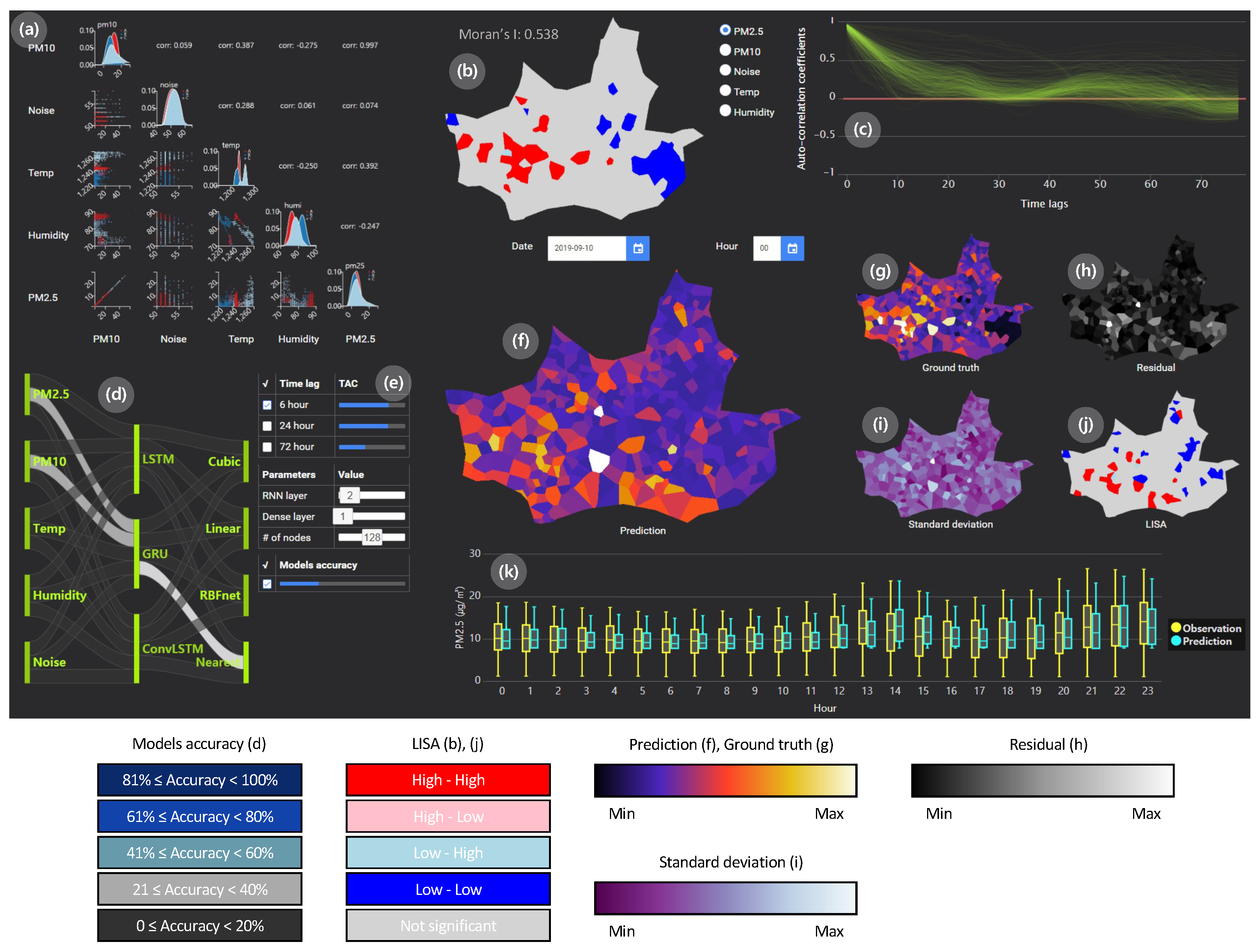
Our spatiotemporal data prediction modeling system, as shown in Figure 1, is a web-based application developed under the Flask framework, and visualization modules are implemented using D3.js. In the back-end, the prediction network models, such as LSTM, GRU, and Convolutional LSTM, are implemented with Python. Figure 1 presents our air pollutant prediction modeling system that enables us to compare spatiotemporal data prediction models and investigate the prediction performance. In Figure 1a, the scatterplot shows the correlation and probability distribution between input variables. We compare five input variables to capture the correlations and data distributions and observe that ${\mathrm{PM}}_{2.5}$ and ${\mathrm{PM}}_{10}$ are highly correlated. The system also presents spatial autocorrelation (Moran’s I) in (b), where LISA is visualized. We recognize high–high and low–low LISA as clusters. The temporal autocorrelation is plotted in (c). We recognize that the temporal autocorrelation of ${\mathrm{PM}}_{2.5}$ becomes weaker as time goes on. The Sankey diagram supports the modeling of the spatiotemporal prediction by combining features, deep learning models, and interpolation models, as shown in Figure 1d. We set the prediction parameters for the models in (e). Here, we set the time lag and deep learning parameters. The interpolated prediction with the nearest neighbor is visualized in (f), where we see the predicted values over the global area. The observed ground truth data are visualized in (g), and the prediction errors are visualized in (h). The standard deviation of prediction over time is presented in (i). The LISA is shown in (j). The box plots represent the temporal predictions compared to the actual observed values in (k).

5.1. Analysis Based on Correlation and Time Lag Settings at Initial State

First of all, the correlations between variables can be identified in the scatter plot matrix in (a). The scatter plot shows the features that correlate strongly with the ${\mathrm{PM}}_{2.5}$ that we attempt to predict. The Pearson correlation coefficient between ${\mathrm{PM}}_{2.5}$ and ${\mathrm{PM}}_{10}$ is close to 1, and the scatter plot shows a strong linear correlation, which confirms that ${\mathrm{PM}}_{10}$ has the highest correlation with ${\mathrm{PM}}_{2.5}$. Therefore, we can attempt to predict ${\mathrm{PM}}_{2.5}$ by inserting ${\mathrm{PM}}_{2.5}$ and ${\mathrm{PM}}_{10}$ features together in the GRU network and the LSTM network. Our system supports three time lags as an input time range, including 6, 24, and 72 h. The results are summarized in

Table 1. Prediction accuracy of different time lags and models with ${\mathrm{PM}}_{2.5}$ and ${\mathrm{PM}}_{10}$ for gated recurrent units (GRU) and long short term memory (LSTM) with mean absolute percentage error (MAPE).

Selected Features	Model	Time Lag (h)	MAPE (%)
${\mathrm{PM}}_{2.5}$	GRU	6	69.4
		24	89.6
		72	72.9
${\mathrm{PM}}_{10}$	LSTM	6	70.5
		24	83.0
		72	72.2

. Overall, it is difficult to tell that all six network models have good predictive performance. Note that we observe the high correlation between ${\mathrm{PM}}_{2.5}$ and ${\mathrm{PM}}_{10}$ within our data, and this is also reported in the study by Zhou et al. [54].

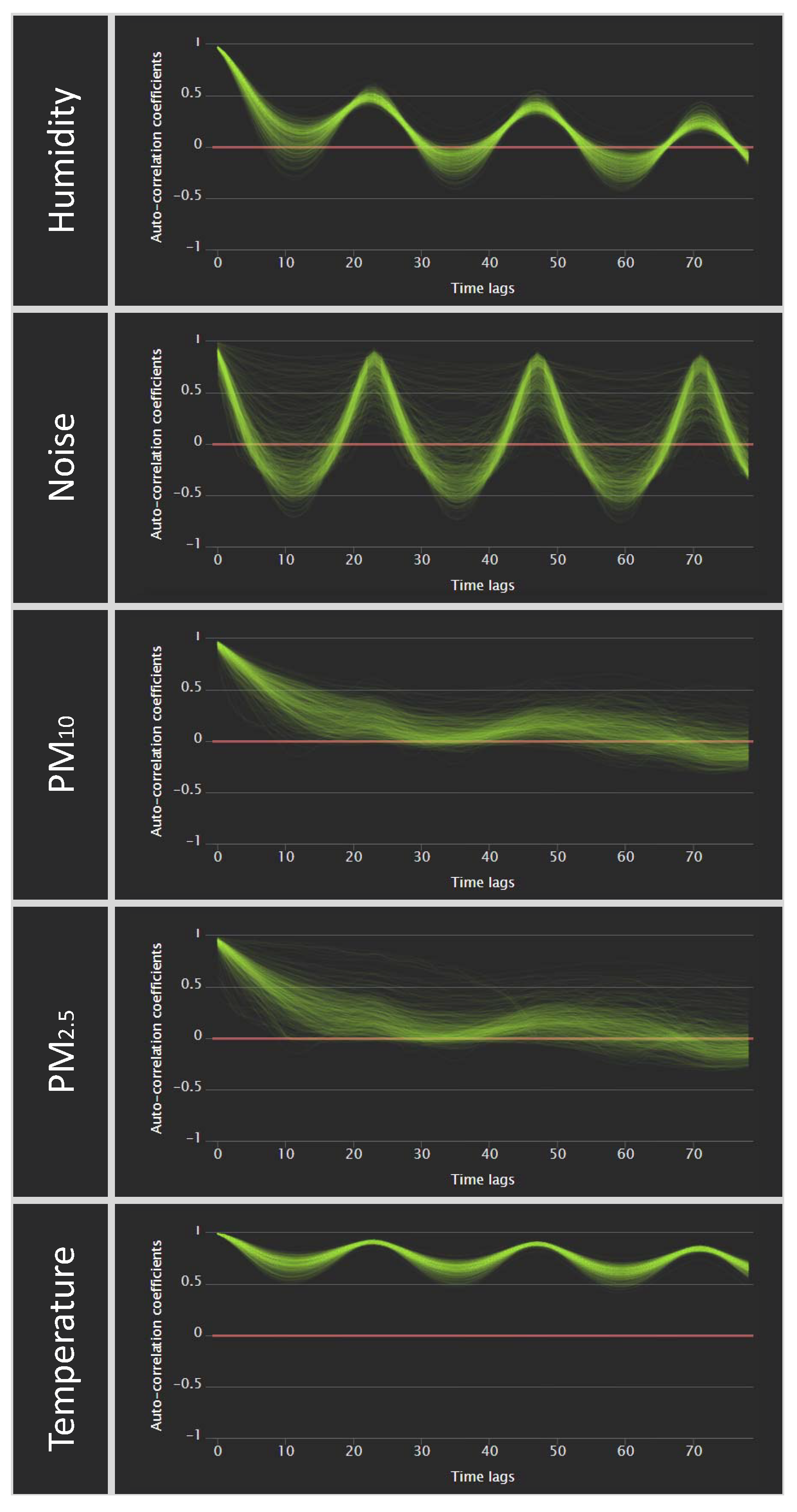
Now, we compare the model performance with different time lags. In both GRU and LSTM networks, when only the parameters of ${\mathrm{PM}}_{2.5}$ and ${\mathrm{PM}}_{10}$ are selected, setting the time lag to 6 h produces lower MAPE than 24 or 72 h. Since the visualization shown in Figure 2 is proposed to set an appropriate time lag, we check that the autocorrelation of each variable changes according to the time lag. We observe the temporal autocorrelation graphs of ${\mathrm{PM}}_{2.5}$ and ${\mathrm{PM}}_{10}$ in Figure 2 to infer the cause for these results. Since the temporal autocorrelation of ${\mathrm{PM}}_{2.5}$ and ${\mathrm{PM}}_{10}$ has a major decreasing trend, we can interpret it as the accuracy for a long time lag tends to decrease. In other words, when only two variables are used, including much data from a past time, it may degrade the prediction performance. We can try two approaches to improve the performance of the GRU and LSTM. First, the models are fixed with GRU and LSTM and features are reselected for the training. Second, we fix the selected features and apply another model, such as the ConvLSTM.

5.2. Analysis Based on Different Feature Selection

When we reconsider the feature selection, we need to identify the problem with the selected features. The selected features, ${\mathrm{PM}}_{10}$ and ${\mathrm{PM}}_{2.5}$, have a strong linear relationship. Therefore, the ${\mathrm{PM}}_{10}$ information is almost similar to the ${\mathrm{PM}}_{2.5}$ information. If duplicate or nearly similar information is included in the input, the information may be insignificant in the prediction. Therefore, we train ${\mathrm{PM}}_{2.5}$ again with temperature and humidity features, which have high linear coefficients next to ${\mathrm{PM}}_{10}$. The results are summarized in

Table 2. Prediction accuracy of different time lags and models with ${\mathrm{PM}}_{2.5}$, temperature, humidity for gated recurrent units (GRU), long short term memory (LSTM) and mean absolute percentage error (MAPE).

Selected Features	Model	Time Lag (h)	MAPE (%)
${\mathrm{PM}}_{2.5}$ Temperature Humidity	GRU	6	45.4
		24	43.0
		72	49.9
	LSTM	6	49.1
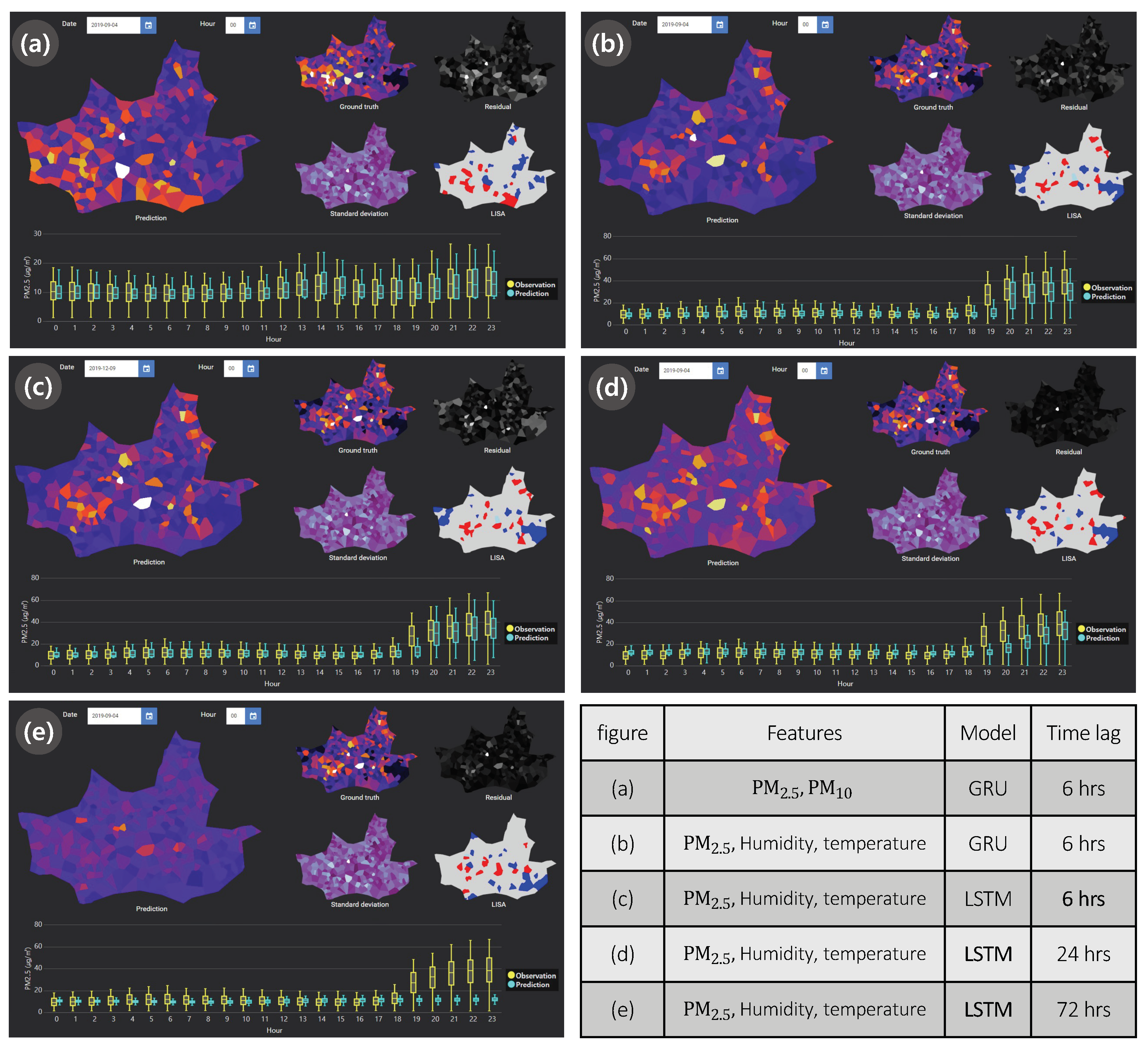
		24	59.6
		72	82.9

and visualized in Figure 3. We observe that the model with ${\mathrm{PM}}_{2.5}$, humidity, and temperature produces more accurate prediction than one with only ${\mathrm{PM}}_{2.5}$ and ${\mathrm{PM}}_{10}$ as presented in Figure 3a,b. The fixed model with the same features predict ${\mathrm{PM}}_{2.5}$ differently according to the time lags, as shown in Figure 3c–e. Although the average MAPE with the time lag of 6 h is lower than one with the time lag of 24 h, we observe that the time lag of 24 h produces lower errors overall in the map visualizations.

In the results after selecting the new feature set, we observe that the MAPE becomes smaller, compared to the previous feature selection. One reason for this is that duplicated information, as previously suspected, may somewhat degrade the prediction performance. We can also see that the model performance according to the time lag is stable in the case of GRU. However, in the case of LSTM, it can be seen that the accuracy decreases significantly as the time lag increases. Therefore, the GRU designed in this paper can be interpreted as being more robust to the past data than LSTM.

5.3. Analysis Based on Different Deep Learning Network

In this test, we fix the features and choose another model, ConvLSTM. Only the ${\mathrm{PM}}_{2.5}$ and ${\mathrm{PM}}_{10}$ features are selected as input features of the ConvLSTM, and the time lag is set to 6 h for the training. The MAPE of ConvLSTM with only ${\mathrm{PM}}_{2.5}$ and ${\mathrm{PM}}_{10}$, and with 6 h of time lag is 34.4%, which is lower than those of the GRU and LSTM networks. We can refer to Figure 1b to see why the predictive performance is better when using a model reflecting the spatial information. In (b), Moran’s I for ${\mathrm{PM}}_{2.5}$ is 0.538, which shows a relatively significant spatial correlation. Since ${\mathrm{PM}}_{2.5}$ has high spatial autocorrelation, we expect that the predictive performance is better when considering spatial information.

5.4. Review of Predictions by Feature and Network Selection

We also train ConvLSTM with three features, including temperature, humidity, and ${\mathrm{PM}}_{2.5}$, which are selected in the temporal predictive modeling in Section 5.2. The MAPE of ConvLSTM with the three features and 6 h of time lag is 21.9%. After reselecting the features, we can see that predictive performance is better. ${\mathrm{PM}}_{2.5}$ and ${\mathrm{PM}}_{10}$ are very similar features. As seen in Section 5.2, the spatial overlap may also reduce the prediction performance. Since the spatial information of each feature is different, the spatial correlation of the prediction result may also be different. Therefore, in the spatiotemporal prediction deep learning modeling process involving spatial factors, it is worth exploring how significantly the spatial information of a feature can affect the prediction.

We attempted to interpret the prediction results for each case as we stepped through the changes of features, time lags, and deep learning models. The proposed system enables deep learning modeling with spatiotemporal data and supports interpreting the causes for the results. During the modeling process, we investigate the prediction results of deep learning models, improve our understanding of the data, and explore the deep learning models faster. In particular, during the process of analyzing the prediction results of the deep learning model with spatiotemporal data, efficient feature selection can be performed by comparing not only the correlations between variables, but also the spatial and temporal correlations.

6. Discussions

In this paper, we propose an approach to select the appropriate features and deep learning model by analyzing correlations, spatial correlations, and temporal correlations for spatiotemporal data prediction. We evaluate our system with spatiotemporal air pollution data to generate the prediction model. We take the past data ($t_1,...,t_{n-1}$) as input and predict the current data at $t_n$ as an output. The prediction results are compared in the map visualizations. The evaluation in Section 5 is intended to perform the deep learning modeling procedure to improve the prediction results through the system. Note that we show the modeling procedure rather than the best results in this paper. The limitations of our approach are in the following.

For feature selection, our system provides the Pearson correlations between variables, temporal autocorrelation with the time lag, and spatial autocorrelation with LISA visualization. However, the extension to spatial filtering and feature extraction during the data analysis can enhance the quality of feature selection. Although our approach can be useful for identifying and predicting global trends in the overall data, our system tends to neglect the local characteristics. For example, we can filter the areas by considering geographic characteristics and environmental conditions. In the case of ${\mathrm{PM}}_{2.5}$, the frequency of occurrence may vary according to the density of factories in neighboring areas, and the diffusion of ${\mathrm{PM}}_{2.5}$ may be changed by mountains or high-rise buildings in nearby areas [55]. We plan to add spatial filtering and apply feature extraction techniques, such as PCA, LDA, and t-SNE.

From a deep learning perspective, we trained the data using LSTM, GRU, and ConvLSTM and compared the predictive performance with the spatiotemporal relationship. According to recent research [44,45,46,47,55], various network structures extended from the RNN structure were investigated as a technique for predicting spatiotemporal data. Although not included in this study, DCRNN (diffusion convolutional recurrent neural network) [56] can be used to predict spatiotemporal data, using directed graph data. This paper utilizes data obtained from irregular discrete stations, rather than grid or known topological data. Such discrete data may be distorted in the connection between features in the process of converting them into a graph structure. When converting from discrete data to the graph structure, the relationship between features determines the weight of the graph. However, it is difficult for us to find the relationship between features from discrete data. After studying the feature selection technique with the feature extraction techniques, we plan to investigate to transform the extracted feature into a directional graph form and apply it to the DCRNN in the future.

The purpose of this study is to examine whether prediction performance degradation is due to feature selection or spatiotemporal correlation. Therefore, we train the data with fixed deep learning hyperparameters such as batch size, loss function, and optimizer. However, setting up appropriate hyperparameters in deep learning is a critical factor in improving predictive performance. Therefore, we need to analyze the influence of hyperparameters on spatiotemporal prediction in the future.

We apply the nearest, linear, and cubic interpolation to spatially interpolate and compare the predictions of the deep learning models as postprocessing. However, these techniques do not work correctly for irregularly distributed stations. To overcome this problem, we can consider applying the RBF network, which is a kind of artificial neural network. The RBF network is calculated using the radial basis function as an activation function and is applied for functional approximations, time series prediction, and classifications [42]. The RBF network can be added ahead of the ConvLSTM neural network as additional layers. This model has the benefit of being able to discard postprocessing for the visualization. We do not need to create image data sets from the spatiotemporal data measured from discrete stations. Therefore, we plan to apply the RBF network to the ConvLSTM neural network in the future.

7. Conclusions

In this paper, we proposed a visualization system that can analyze deep learning models. We proposed an approach to select the appropriate features and deep learning model by analyzing correlations, spatial correlations, and temporal correlations for spatiotemporal data prediction. We analyzed deep learning based prediction model with an air pollutant data set, which represents an irregularly distributed spatiotemporal data set. Our system allows us to explain the reason for the low performance of a deep learning model in the aspect of spatial and temporal correlations. We believe that our approach supports us in understanding the parameter settings and improving deep learning models for spatiotemporal data. It is possible to extend our system to include more deep learning models and explain the predicted results, which is crucial in deep learning research. However, our model has some limitations, including the lack of feature extraction and the hyper parameter setting of deep learning networks. To overcome this problem, we plan to add spatial filtering, apply feature extraction techniques, including PCA, LDA, and t-SNE, and apply a DCRNN architecture by transforming the extracted feature into a directional graph form. We also plan to apply the RBF network to the ConvLSTM neural network in the future.