Article

Optimization Procedure for Computing Sampling Time for Induction Machine Parameter Estimation

Faculty of Electrical Engineering, Computer Science and Information Technology Osijek, J.J.Strossmayer University Osijek, Trpimirova 2B, 3100 Osijek, Croatia
*
Author to whom correspondence should be addressed.
Appl. Sci. 2020, 10(9), 3222; https://doi.org/10.3390/app10093222
Submission received: 26 March 2020 / Revised: 27 April 2020 / Accepted: 28 April 2020 / Published: 6 May 2020
(This article belongs to the Special Issue Modeling, Design and Control of Electric Machines)

Abstract

:
This paper presents a method for selecting the sampling time for induction machine parameter estimation from the machine line start measurements. the metaheuristic optimization method is used to find the optimal Prony exponential series approxiamtion of the line start transient current. From the optimal approximation, poles of the linearized induction machine model are computed and used to determine the optimal sampling time. the results show that sampling frequencies needed for parameter estimation are much lower than 1–15 kHz commonly used today. This reduces the necessary amount of collected data and the computing power needed for the estimation. the optimal sampling time is computed for the simulated and for the measured data. Referenced parameter estimation technique is tested for the measured transient showing benefits of using the optimal sampling time.

1. Introduction

A well known problem in induction motor (IM) control is estimating the correct parameters of the motor. The fact that determining induction machine parameters is not an easy task yields a new research objective about the IM parameter estimation that has been thoroughly reviewed in [1,2].
A part of the experiment design for parameter estimation is also selecting the sampling intervals for the measured quantities. Research in statistics approaches this problem seriously, developing different methods for selecting sampling intervals that are usually custom made for combinations of model, equipment, excitation and noise levels to obtain the best possible parameter estimates. This is evident from the basic textbooks like [3,4], but hard to use with IM experiments due to the wide range of motor parameters, different estimation methods and equipment used.
In applications to the IM parameter estimation, the selection of sampling time is almost always based on equipment capability or some other algorithm execution cycle (such as control algorithm). Most commonly the parameter estimations use the data acquired with sampling frequencies from 1 kHz to 15 kHz depending on the application as seen in [5,6,7,8]. The authors have found only one paper [9] that allows for adapting of the sampling period, but its motivation was solving the computational problem of time averaging. One more paper [10] uses 100 Hz frequency to adapt the parameters of the IM without the explanation why is it so low.
Naturally, selecting low sampling frequency may lead to problems with Nyquist sampling boundaries, so many authors choose the highest possible sampling rates. This results in having large data sets for offline processing that can be time and memory consuming, or introduces noise sensitivity and need for very fast computing power in case of online estimation.
The term optimal sampling time found in literature is quite rare. Paper [11] deals with selecting the optimal sampling time to improve the accuracy of the mean and RMS (root-mean-square) value computation for multisine signals and the paper [12] goes further and determines the optimal sampling for Gauss-Markov scalar processes. The latter paper is interesting in sense of this research since it shows that the optimal time sampling is also related to the window size of the collected data, a problem that this paper also takes into account. Also, the paper [12] discusses the optimal sampling time as the smallest sampling time, based on the variance of the estimated parameters, while it also notes that reducing sampling time beyond a certain point does not give significant improvement to the estimation results.
A disscusion more suited to this research field is from [13]. There the authors analyse the optimal sampling time with respect to the optimal control law for linear systems. That paper also mentions the term quantization in the time domain, which is mainly viewed as a negative influence on controllers. The work presented in paper by Elia in chapter 32 of [14] utilizes the time and amplitude quantization to stabilize unstable systems and refers to optimal sampling time from that point of view.
From these references, the term optimal sampling time is hard to define without a specific purpose that the optimal sampling time refers to. Over 30 years ago, in [15] the authors dealt with the problem of optimal sampling time in general system parameter estimation itself. In this paper authors have derived a criteria for sampling time selection for linear deterministic systems. Few years later, in [16] the authors present the optimal sampling time for stochastic systems, mainly giving the Kalman filter optimal sampling time as a result.
In this paper the authors follow the criteria for optimal sampling time given by Sinha and Puthenpura in [15]. This criteria is given for linear systems, whereas IM model is nonlinear. In order to apply the criteria by Sinha, the linear system poles must be known in advance. Naturally they are not, nor are the parameters of the linearized system from which they can be computed. Therefore we propose using the Prony method to estimate the poles from the line start experiment of the IM, that can be used for Sinha method of optimal sampling time. Application of the Prony method to the approximation of induction machine nonlinear transient is a challenge that is addressed in this paper by optimal segmenting and decimation of the collected data. This is done to obtain intervals of data where the Prony approximation remains accurate. The paper is structured as follows: the second section introduces the parameter estimation problem this paper refers to and introduces the mathematical background for fitting the data by Prony exponential series to determine the linear system poles. The third section describes the application of the mentioned technique to the nonlinear induction machine transient data. The computed poles are then used to compute the optimal sampling time in Section 3.4. Section 4 shows the simulation and experimental application results.

2. Parameter Estimation Problem and System Poles

In this section the parameter estimation problem that is applied to the induction machine nonlinear model is introduced. The optimal sampling time is computed with the aim to improve the solution of this problem. Subsequently, the procedure to determine linear systems poles is presented as a fundamental step in determining the induction machine optimal sampling time.

2.1. Parameter Estimation Procedure

For the system described by state space model (Equation (1)):
d d t x = f ( x , u | Θ ) y = g ( x , u | Θ )
where f : R n × m R n and g : R k × m R k are state and output functions with state variables x R n , output variables y R k , and input variables u R m and where Θ = θ 1 θ 2 θ l S R l is the parameter vector, the parameter estimation problem is defined as follows.
Given the discrete observed (measured) data y [ i ] and known inputs u ( i ) at time instants i = p T s , p = 1 , 2 , 3 q , with the step time T s that corresponds to the sampling frequency f s = 1 T s , the problem of finding the optimal parameter set Θ ^ that minimizes (or in some cases maximises) the given criterion function J C ( Θ ) is called the parameter estimation problem for nonlinear state space models.
The criterion function J C ( Θ ) is most commonly selected as the sum of squared residuals (also known as least squares criterion) presented in Equation (2), but there are cases where different functions such as maximum likelihood criterion, or least absolute differences criterion are used. More on criteria functions can be found in [17].
J C ( Θ ) = p = 0 q [ y [ p ] y ( p T s ) ] 2
In Equation (2) the y [ p ] are the measured samples of the output variables and the y ( p T s ) are the computed output variables obtained by some method of computation from Equation (1).
The problem of parameter estimation is therefore separated into two different steps. The first step is computing the dynamical system response y ( p T s ) and the second is solving the optimization problem shown in Equation (3).
Θ ^ = argmin Θ S J C ( Θ )
Computing the system response y ( p T s ) can be done by numerical solving of Equation (1) with a trial set of parameters Θ = Θ t r i a l , by computing the response analytically or by estimating the response based on observations ( y [ p ] ) with methods such as Kalman Filters (extended Kalman for nonlinear systems).
Solving the optimization problem (Equation (3)) is completed using one of the availabel and applicable optimization methods that can be gradient based or numerical methods for approximating global minima.

2.2. Determination of the Linear System Poles

The system described by Equation (1) with f ( x , u ) = A x + B u and g ( x , u ) = C x , where A , B and C are matrices of appropriate dimensions is a linear state space system.
For the specific case with the initial condition x ( 0 ) = 0 and for systems with single input that is a Dirac delta function u = δ , the linear system response can be expressed in terms of the state transition matrix Φ = e A t in the Equation (4).
x ( t ) = 0 t Φ ( t τ ) B δ ( τ ) d τ = Φ ( t ) B
The state transition matrix Φ can be computed based on modal decomposition of the state matrix A such that:
Φ = W e Λ t W 1
where e Λ t = diag [ e λ 1 t e λ n t ] is the matrix exponential of the A matrix eigenvalues λ i , and W is the matrix of corresponding eigenvectors.
Since the system output is a linear combination of states and since the state transition matrix is defined using the matrix exponential and system eigenvalues (for further details see [18]), it can be concluded that the i-th system output under given conditions is the sum of modal exponentials:
y i = j = 1 k G i j exp ( λ i t )
where G i j are constants determined from the initial conditions of the output variables and λ i is the system i-th egienvalue.
The Prony method approximates a measured signal with the sum of damped complex exponentials. It can be used for determining the system eigenvalues directly from the measured impulse response.
The general discrete n-th order Prony approximation y ^ [ p ] of the measured signal y [ p ] is represented in Equation (7)
y ^ [ p ] = i = 1 n R i exp ( j ϕ i + λ i p T s ) = i = 1 n R i e j ϕ i z i p
If it is assumed that G i j = R i j e j ϕ i j is constant the Equation (6) becomes the classical expression of the Prony approximation of a measured signal.
An efficient and computationally stable method for determining the poles of the damped complex exponential approximation is to use the matrix pencil method introduced by Hua and Sarkar [19,20]. This method turns the problem of finding the eigenvalues into problem of solving for the matrix pencil eigenvalues. The method is explained in mentioned references and only its application is presented here.
The matrix pencil can be formed using the Hankel matrix H for the i-th system output measurement set y i = y i [ 1 ] y i [ q ] .
H = [ y i [ 1 ] y i [ n ] y i [ n + 1 ] y i [ 2 ] y i [ n + 1 ] y i [ n + 2 ] y i [ q n ] y i [ q 1 ] y i [ q ] ]
Written in terms of collumn vectors h the matrix is:
H = [ h 1     h n   h n + 1 ]
a matrix pencil P is formed as:
P = H l + z H r
where:
H l = [ h 1 h n ] H r = [ h 2 h n + 1 ]
With defined matrix pencil P , the equation for discrete eigenvalue computation is formed as:
P = H l + z H r = 0
Solving Equation (12) for all z yields the discrete system eigenvalues. In order to compute the eigenvalues one must solve Equation (12) by means of singular value decomposition since the matrices H l and H r are rank deficient. Therefore the eigenvalues are just an approximation of the real system eigenvalues.
With determined discrete poles z k , k = 1 n , the procedure from classical Prony method found in [21] is used to find damped exponentials R i j e j ϕ i j .
In this paper entire complex exponential approximation is used for evaluating the fitness of the exponential series to the measured data, but only the eigenvalues are used in computing the optimal sampling time.

3. Optimal Induction Machine Poles and Sampling Time

3.1. Induction Machine Model

The induction machine model is well known today. The model is derived by transforming the circuit equations from three phase system into two component system using the Park transformation, details found in [22,23]. To create a single input state space model for the simplest implementation of the procedure described in the continuation of the paper, the IM model is written in the voltage oriented ( v q = 0 ) rotating (dq) reference frame with fluxes as state variables:
d d t ψ s = v R s G s ψ s R s G m ψ r ω k T r ψ s d d t ψ r = R r G r ψ r R r G m ψ s ( ω k p ω ) T r ψ r d d t ω = G m J 3 2 p ( ψ s d ψ r q ψ s q ψ r d ) 1 J M L
The notation in Equation (13) is: v = v d 0 T dq components of stator voltage, ψ = ψ d ψ q T dq components of fluxes, subscripted ‘s’ for stator and ‘r’ for rotor quantities, R s —stator resistance, R r —rotor resistance, ω k —the dq reference frame rotating speed, grid synchronous speed in this case, ω —the actual rotor speed, p—number of pole pairs, J—rotor inertia, M L —the load torque, T r —the rotational matrix defined in Equation (14) and parameters G are the elements of inverse of machine inductance matrix L defined in Equation (15) with L s = L l s + L m , L r = L l r + L m , where L m is the main magnetizing inductance and L l s , L l r are the stator and rotor leakage inductances.
T r = [ 0 1 1 0 ]
G = [ G s 0 G m 0 0 G s 0 G m G m 0 G r 0 0 G m 0 G r ] = [ L s 0 L m 0 0 L s 0 L m L m 0 L r 0 0 L m 0 L r ] 1

3.2. Linearized Induction Machine Model

For any nonlinear state space model operating at the stationary point x 0 with the stationary input u 0 , the response for small change in input variables Δ u can be approximated using the linearized form of the model. The linearized form is represented in Equation (16).
d d t Δ x = A Δ x + B Δ u Δ y = C Δ x + D Δ u
With:
A = x f | x = x 0 u = u 0 C = x g | x = x 0 u = u 0 B = u f | x = x 0 u = u 0 D = u g | x = x 0 u = u 0
Particular interest of this paper is in the matrix A of the linearized induction machine model. If the known simplification ( d d t ω = 0 ) found in [23] is used, the right hand side of the rotational motion equation of the model in Equation (13) becomes zero. Using this assumption, which is valid if the current transients in the model are much faster than the speed transients, the linearized matrix A of the induction machine model in Equation (13) is:
A = [ R s G s ω k R s G m 0 0 ω k R s G s 0 R s G m 0 R r G m 0 R r G r ω k p ω 0 ψ r q 0 0 R r G m p ω 0 ω k R r G r ψ r d 0 0 0 0 0 0 ]
The poles λ of the linearized system described by Equation (16) are the eigenvalues of the matrix A . The k-th discrete pole ( z k ) of the system, used for discrete and recursive computation, is calculated using the k-th continuous eigenvalue ( λ k ) and discrete sampling time T s as:
z k = exp ( λ k T s )
Since the IM model is nonlinear, the only discussion about the poles location can be in context of linearized models. In order to apply any method for selection of optimal sampling time based on poles location, one must know poles a-priori. If poles are known from the system model, the parameter estimation is not necessary. Therefore the problem of finding optimal sampling time for parameter estimation as described by [15] can be rephrased as a problem of determining the system poles without the knowledge of the system and the optimal sampling time.
The procedure for finding the system poles by Prony approximation is described, but it is not straightforward applicable to the measurements of the IM transient. Some considerations need to be made: the IM model is nonlinear, the measured transient is not expected to be an impulse response.
In this paper these issues are overcome by applying the procedure to the measurements of the direct line start of an IM. This is effectively a step response of a nonlinear system with x ( 0 ) = 0 . The response around the initial condition can be represented by the linearized model, but as time goes on, the linearized response and real nonlinear response becomes very different. For observing the small interval around the initial condition point, the step function can be thought of as a finite impulse.
The question that arises is how long is the initial interval, and how many points, sampled at what rate are needed to achieve the accurate pole estimation via Equation (7). This paper proposes the use of an optimization technique, described in the following subsection, to determine these factors.

3.3. Optimal Poles of Induction Machine

The application of the method for obtaining system poles from the IM line start is formed as an optimization problem. The general optimization problem is formulated as finding the vector variable x that minimizes the scalar objective function f ( x ) , subject to equality and inequality constraints presented using vector functions g ( x ) and h ( x ) that define the set S of all admisible values for x . The general optimization problem is presented in Equation (20).
f ( x ) min . x ^ = argmin x S f ( x ) subject to constraints g ( x ) = 0 h ( x ) 0
The optimization problem for obtaining the IM poles by fitting Prony complex exponential series to the measured line start transient is derived in the following paragraphs.
The observed value for computing the Prony complex exponential approximation is the d-axis current, y = i d , in the voltage oriented reference frame. Since the machine model given by Equation (13) is fifth order, the total number of elements in the sum and the order of the estimated model by Equation (7) is n = 5 . Therefore, the 5 eigenvalues of the linearized model can be approximated.
Given the limited order of the estimated damped exponentials, it is not expected that the entire transient can accurately estimated by Equation (7). Therefore, the transient is divided into shorter intervals, and the aim is that each interval is short enough for the accurate estimation with the fifth order model. This criteria gives the interval duration where the nonlinear transient can be approximated with the fifth order damped complex exponential sum. The total number of observations in the interval is noted q i n t , with the reminder that the total number of observations in the measured set is q. The total number of intervals the data are separated into is described by Equation (21) (rounded to the nearest integer).
N i n t = q q i n t
Secondly, the transient is sampled at the sampling rate T s , m i n , the fastest sampling rate possible. When fitting the data with model from Equation (7) it is assumed that less data is needed. Therefore a decimation factor d N is introduced such that the decimated sampling time is T s , f i t = d T s , m i n . Now selecting every d-th element of the original measured set (down-sampling) can provide the data reduction. The original measured set y [ p ] is decimated to y d [ p ] = y [ d p ] , and with decimated data, the new interval size is q d = q i n t / d .
With interval size q i n t and decimation factor d introduced, the optimization problem can be formed. The optimization objective function is presented in Equation (22)
J e s t = w = 1 N i n t M S E w
where the M S E w is the mean sum of squared residuals for w-th interval:
M S E w = 1 q d r = ( w 1 ) q d w q d ( y d [ r ] y ^ d [ r ] ) 2
and where y ^ d [ r ] is computed by fitting the decimated data y d [ r ] from the interval ( w 1 ) q d < r < w q d with damped complex exponentials from Equation (7) by the procedure described in Section 2.2.
The decision variables of the optimization are Γ = d q i n t and the optimization problem is to find the optimal Γ ^ that minimizes the objective function, Equation (22), subject to constraints Γ S N 2 . The set S is the set of all permissible integer values of the decision variables, bounded by the lower and the upper bound for each decision variable. The total optimization problem is presented in Equation (24).
J e s t ( Γ ) min Γ ^ = argmin Γ S N 2 J e s t ( Γ ) subject to constraints Γ L B Γ Γ U B
where Γ L B = d L B q i n t , L B and Γ U B = d U B q i n t , U B are the lower and upper bounds to the decision variables search area S N 2 .
For the optimal Γ ^ the damped complex exponentials fit of the very first interval gives the discrete system eigenvalues z k , k = 1 n .
In this paper, the optimization problem (Equation (24)) is solved using commercially availabel MIDACO Solver (mixed integer distributed ant colony optimization) in co-simulation environment with Matlab [24]. MIDACO is a global optimum approximation solver from the class of nature inspired metaheuristic algorithms (such as genetic algorithm, particle swarm optimization, etc.). More on MIDACO can be found in the research made by the creators of the program [25]. Only necessary settings for the MIDACO Solver are the constraints to the variable search area. The co-simulation environment uses Matlab to compute the objective function value and MIDACO to compute the next generation of the decision variables based on the optimization algorithm.

3.4. Optimal Sampling Time

When motor poles are calculated by fitting the damped complex exponentials to the decimated and interval divided data, the computation of the optimal sampling time is straightforward following the criteria introduced by Sinha [15] and applied in synchronous generator parameter estimation in [26].
The method describes the optimal sampling time as the longest interval T s , o p t for which the Tustin bilinear transformation used to approximate continuous systems with discrete systems is not loosing accuracy.
Put in numbers, given the largest magnitude of the continuous system eigenvalues | λ m a x | , and the sampling time T s , the bilinear transformation holds if
| λ m a x | T s 0.5
Without presenting the details that can be found in [15,26], the optimal sampling time is obtained from the minimum magnitude discrete pole z m i n = | z m i n | e j ϕ z of the system by numerical solving of the Equation (26) for unknown K, and computing the optimal sampling time as T s , o p t = K T s , f i t .
[ | z m i n | 4 K + 2 | z m i n | 2 K cos ( K ϕ z ) + 1 ] 1 / 2 | z m i n | k 2 2 | z m i n | K cos ( K ϕ ) + 1 = 5

3.5. Summary of the Procedure and Computational Complexity

The whole procedure for computing the optimal induction machine sampling time is now summarized:
(1)
Record the line start transient in voltage oriented reference frame, v q = 0 , with the fastest possible sampling time
(2)
Determine the optimal induction machine poles by solving optimization problem (Equation (24)) using the current i d as the observed variable.
(3)
Determine the optimal sampling time factor K by numerical solution of Equation (26), and compute the optimal sampling time T s , o p t .
Solving of an optimization problem by metaheuristic algorithm (MIDACO Solver in our case) and iterative numerical solving of the nonlinear Equation (26) is required for the computation of the optimal sampling time.
The optimization problem also requires solving of Equation (12) by means of singular value decomposition. This is the computationally most demanding step since it is repeated for each interval of the data segmented by the optimization procedure and for each iteration of the optimization. Therefore the requirements crucial to reducing the computation time is limiting the search area of the optimization procedure to reasonable intervals.
Another aspect that seriously impacts the computation time is the original sampling time of the data and the duration of the recorded transient. This determines the total number of the original data samples. Depending on the stage of the optimization and the selected optimization variables, the original sampling time and transient duration alter the dimensions of the Hankel matrix Equation (8). This in turn affects the computational burden of the singular value decomposition solution of Equation (12). Naturally, lower initial sampling time and longer transient duration increase the computation demands.
This paper suggests using the fastest possible sampling time for the best accuracy. However, the sampling times using FPGA based implementations can be reduced to nanosecond intervals which could lead to demanding computation of this procedure, so lowering the initial sampling frequency to commonly used 1–15 kHz is considered good initial sampling from the computation standpoint.
In the examples presented in the following section the boundaries of the optimization are selected very wide. To test the diversity and applicability of the procedure, the simulation example uses large power and inertia motor (132 kW) that has longer line start transient duration. This motor is expected to have the poles in different locations in the z-plane than 4 kW motor used in the experimental example. However, the main reason to simulate 132 kW machine is to obtain the worst case scenario for the computational burden of the algorithm. The computational burden of the procedure is pointed out in the simulation and experiment subsections respectively.
In the simulation, the original sampling time is set to microsecond level which, together with the long transient duration, demonstrates the largest expected computation time of the algorithm. In the measured data application, lower initial sampling (10 kHz) is selected, but the procedure still uses wide boundaries for the optimization variables. This demonstrates the actual computational time for practical use, that could be further reduced using narrower boundaries for the optimization based on experience.

4. Simulation and Experiment

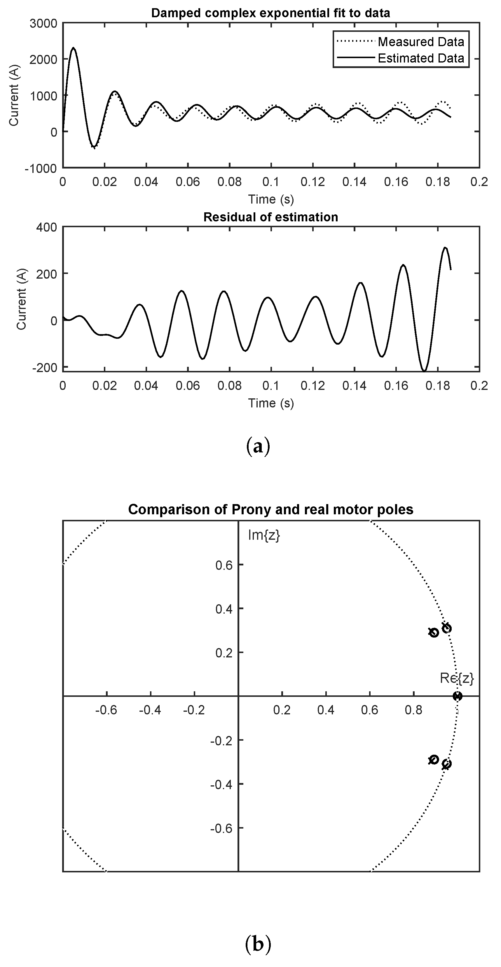
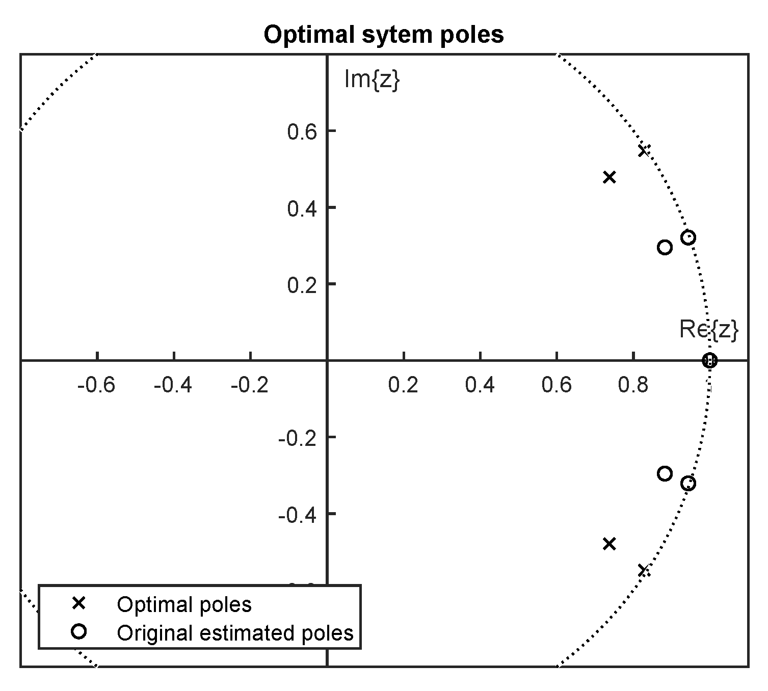
4.1. Application to the Simulated Data

The method is first tested on the simulated data. As mentioned, the method is implemented in Matlab 2018b [24] programming language in co-simulation environment with MIDACO [25]. The motor line start is simulated with Simulink using the model described by Equation (13). Discrete solver is Runge-Kutta and the step size is 1 μ s.
The simulated motor is 132 kW pump motor with parameters R s = 8.9 m Ω , R r = 16.7 m Ω , L l s = 0.2 mH , L l r = 0.2 mH , L m = 14.1 mH , J = 5 kg m 2 .
The optimization variables are constrained with lower and upper boundaries determined by experience of the user and some physical consideration. They are set larger then necessary to demonstrate longest expected computation time. Selecting the boundaries of parameter space for solving Equation (24) is simple, the decimation factor is minimum of one. The maximum decimation is bounded by the maximum significant frequency of the current spectrum. It is chosen as 300 Hz giving the Nyquist frequency F n y = 600 Hz. This corresponds to the upper bound for the decimation factor as d = r o u n d ( T s , m i n F n y ) 1 . The upper bound to the interval size is selected so that the entire original data set can be considered as a single interval. The lower bound is selected so that the data set can be divided into 1000 smaller intervals of 200 data points, effectively giving the smallest interval time of 0.2 ms.
Optimal fit of the damped complex exponentials to simulated data is presented in Figure 1a, and the computed linearized model poles obtained from the damped complex exponentials and the real linearized poles in the first interval obtained from Equation (18) and Equation (19) is presented in Figure 1b. These figures show that the data segmentation and decimation by optimization procedure provides the first interval that is accurately estimated by the Prony exponential series. The estimated poles are accurate enough to be used for computing the optimal sampling time. Therefore no prior knowledge of the motor parameters is required.
The results of the optimization are: decimation factor d ^ = 997 and interval size q ^ i n t = 179,650 . This reduces the the data originally sampled at T s , m i n = 1 μ s to the interval size of 181 samples sampled at T s , f i t = 0.997 ms . Solving the Equation (26) with minimim magnitude pole obtained from the optimization yields the optimal sampling time T s , o p t = 1.774 ms and the discrete poles with optimal sampling time are z o p t = e λ T s , m i n K = e λ T s , o p t = z K . The optimal poles, and the damped complex exponential poles are shown in Figure 2. The figure shows how using the optimal sampling time spreads the poles of the sytem in the z-plane. As is known, reduction of the sampling time asymptotically contracts the poles of a discrete system towards the point (1,0) on the unit circle. This in turn reduces the system robustness to computational errors. Therefore, using the optimal sampling time to spread the poles from the unit circle increases computational stability while preserving the ability to approximate continuous system with discrete versions.
For the presented example, the procedure computation on Intel i7 processor with 16 GB RAM memory it takes about seven minutes to calculate the optimal sampling time. This is the longest computation time expected from this procedure, obtained by very wide bounds for the optimization variables, very fast initial sampling time of 1 μ s and long line start transient due to large simulated motor inertia. Using common initial sampling frequency of (1–15 kHz) dramatically reduces the computation time, as is presented with the experimental data in the following subsection.

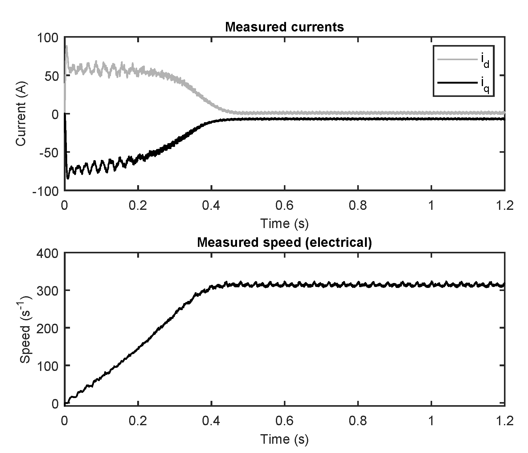
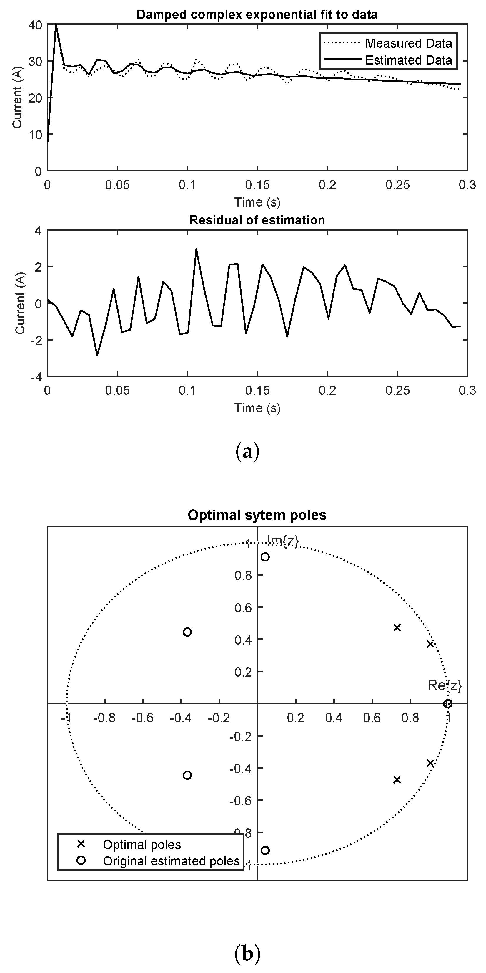
4.2. Application to the Experimental Data

The optimal sampling time procedure is tested on measurement data, and parameter identification procedure is conducted to compare the effectiveness of the procedure with optimal sampling time and original sampling time.
The motor used for the test is the Končar 5AZ112M-4B3, nominal power is 4 kW, and nominal speed 1420 rpm. The motor is delta connected with 380 V/50 Hz line voltage applied directly. The measurements are completed using the IOTECH WaveBook 512 data acquisition system, with Iotech WBK61 voltage sensors and Tektronix A622 current clamps. The initial sampling time is set to the fastest possible sampling with the mentioned hardware configuration, to T s , m i n = 0.1 ms . The measured quantities are shown in Figure 3. It can be seen that the measured data is contaminated with noise which is expected to reduce the quality of the results.
The procedure for obtaining optimal sampling time is tested on measured current i d (voltage oriented reference frame v q = 0 ). The results of fitting the damped complex exponential series to the data is displayed in Figure 4a. Clearly the fit is less accurate than in the noiseless data and the optimal decimation of the measured data is large. The optimal decimation is d ^ = 59 that decimates the optimal interval size of q ^ i n t = 2985 to the q d = 51 . Large decimation also results in the long sampling time for the damped complex exponentials fit to the data (namely T s , f i t = 5.9 ms ). The system estimated discrete poles are shown in the Figure 4b. The figure shows that the heavy decimation of the measured data effects the pole locations so they are scattered even to the left half plane of the z-plane. It is not expected that the discrete IM model can correspond to the continuous for this sampling time. With the estimated motor poles, the procedure for obtaining the optimal sampling time is conducted. The result for optimal sampling is T s , o p t = 1.4981 ms , and the optimal motor poles are also shown in Figure 4b. The optimal sampling time in this case contracts the poles towards the (1,0) point in the z-plane, thus retaining the possibility of discrete approximation of the IM model while keeping them spread far enough to remain computationally robust.
It can be seen that the optimal sampling time for the experimental IM is much higher than the original sampling time used for recording the transient, but it is lower than the decimated sampling time that is used for fitting the data with Prony exponential series. This shows that even if the initial sampling is too slow, one can calculate if the faster sampling is needed as long as the Prony exponential series approximates the data.
In the case of experimental data, where the initial number of samples used for computing is lower and more realistic in regards to applications with IM, the total time to compute the optimal sampling time is averaged at 32.5 s based on 20 repeated runs. This is significant reduction compared to seven minutes in the simulation case that demonstrates realistic expectations of the algorithm demands.

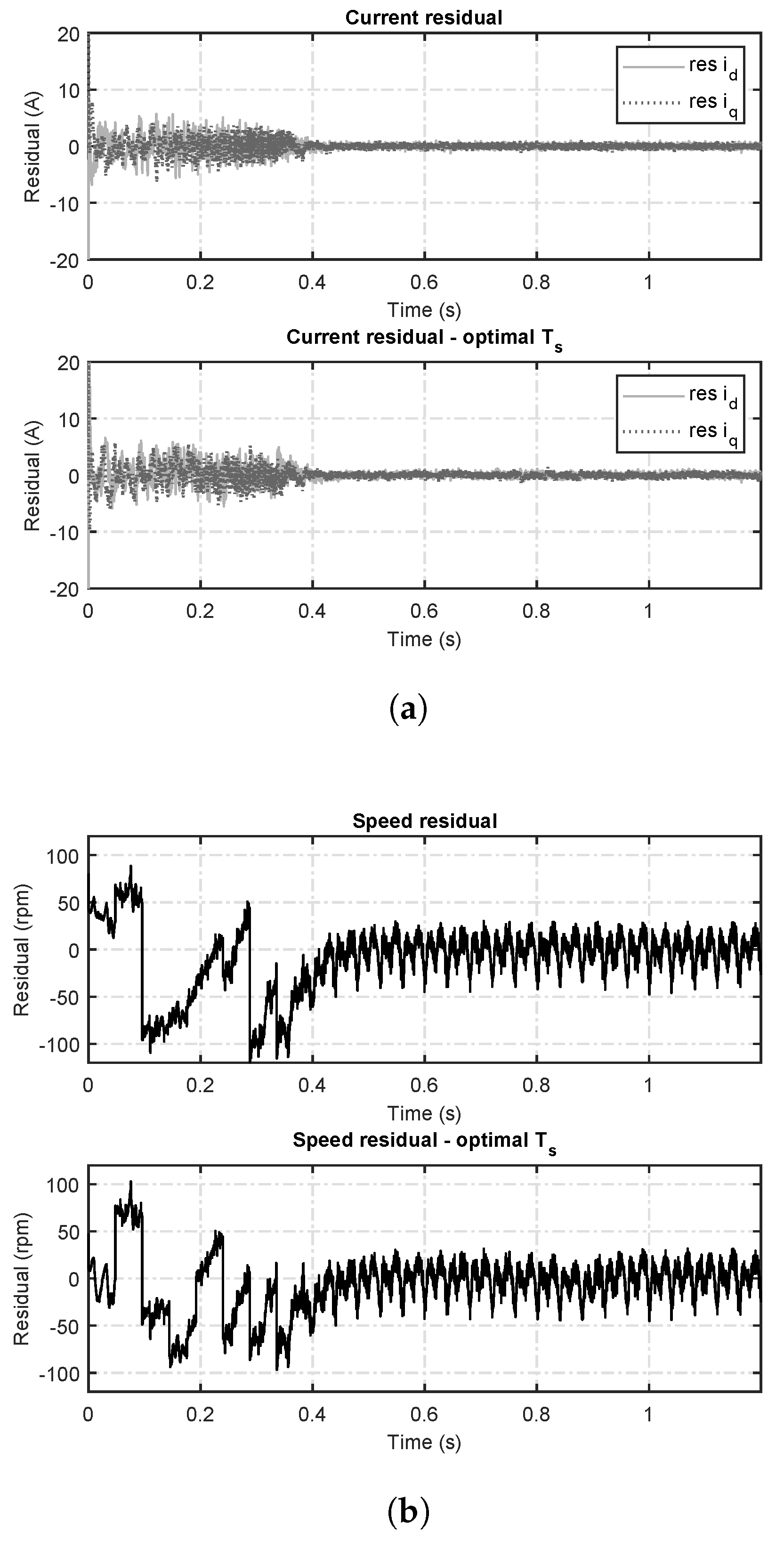
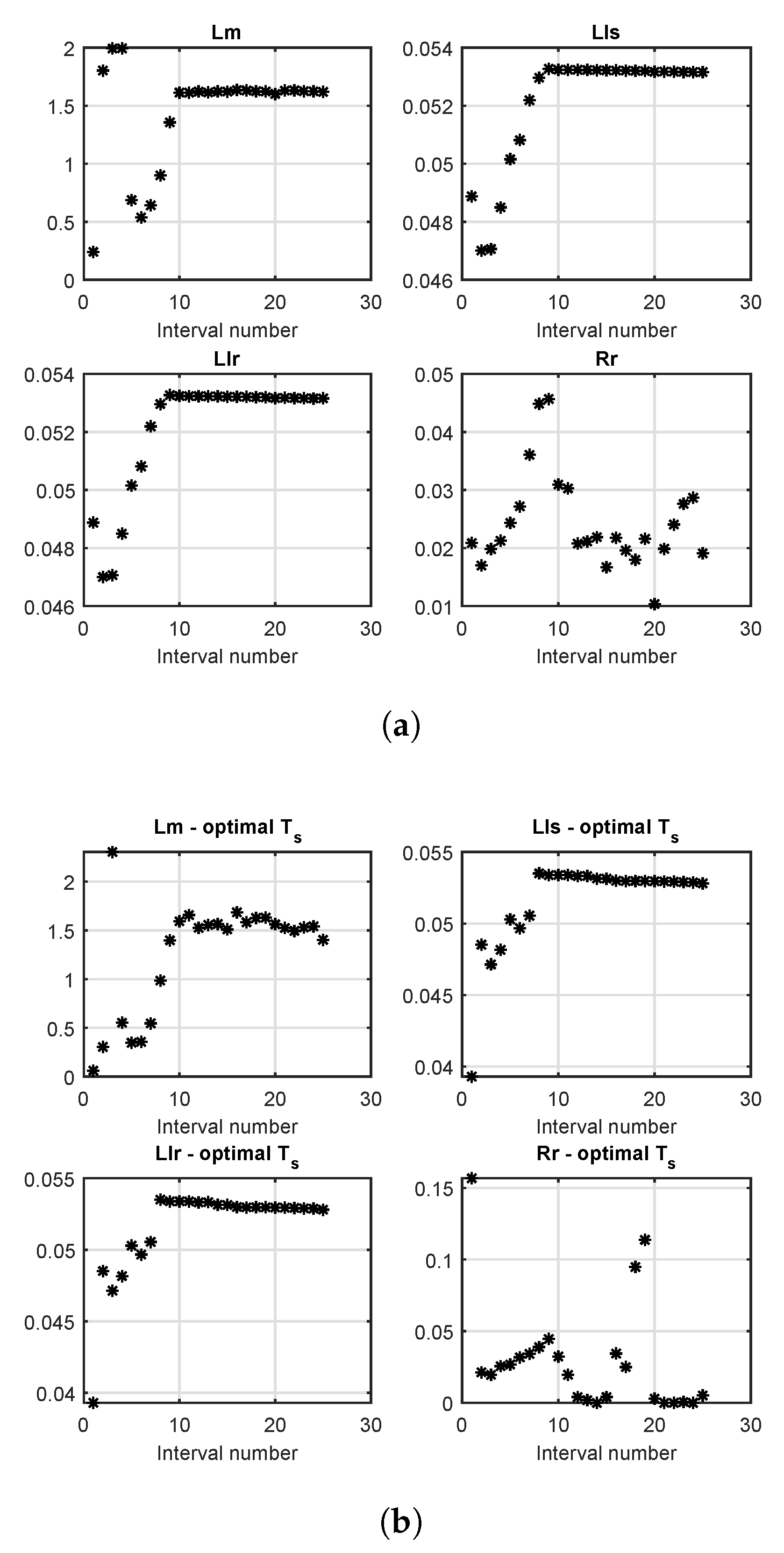
4.3. Testing Optimal Sampling Time on Parameter Estimation

Using the optimal sampling time claims to improve the parameter identification procedures for the motor. To test this claim, a parameter identification procedure is tested for the measured data. The procedure used in this paper is explained in [27]. In brief, the parameter identification procedure uses constrained global optimization to compute the solution of Equation (3), with measured quantities: voltage oriented reference frame currents and rotational speed ( y [ p ] = [ i d [ p ]     i q [ p ]     ω [ p ] ] T ). The model step response is computed by solving the model (Equation (13)) by Runge-Kutta method. This procedure is repeated for the original data set segmented into 25 intervals, thus returning 25 parameter vectors that represent the time varying parameters during IM line start. The parameter vector for each interval is Θ = [ G s     G m     R r G r     R r G r     x 0 T ] T , where the x 0 is the initial condition of state variables (the fluxes, and the rotational speed) for each interval. Input to the system is the peak nominal voltage aligned with the d-axis, and all quantities and parameters used for identification are in per unit system where base voltage is peak voltage, base power is nominal apparent power and base speed is synchronous speed.
The results for parameter identification with original sampling time of T s , m i n = 0.1 ms and with optimal sampling time T s , o p t = 1.4981 ms are shown in Figure 5a,b and Figure 6a,b. Figure 5a,b show the residuals of measured and calculated current and speed and their values calculated from the estimated model with original and optimal sampling time used in estimation. It is clear that the current residual does not show any improvement regarding its quantities or the fact that the aim is to reduce residuals to zero-mean with minimal variance.
On the speed residual the change is noticeable. With the original sampling time the residual of the speed shows bias around 50 rpm in the initial moments of startup (when the actual speed is around 0), and than jumps to −90 rpm after which it is starts to increase but constantly stays biased in the negative values. The optimal sampling time speed residual shows the residual with low quantities during the initial phase thus making smaller error compared to the original. After that it jumps to around 75 rpm (same as with the original sampling time) and drops to negative quantities after 0.1 s. The drop is lower than the original case, and after 0.2 s the residual becomes positive again, thus pulling the entire residual closer to the zero-mean desired shape.
In the steady state, the same performance can be observed for both original and optimal sampling time, where the speed residuals consist of the eccentricity oscillations introduced by the tachometer used for measurement of the speed.
To continue the investigation of optimal sampling time the identified parameters are presented. Figure 6a,b show the parameter values obtained with the original and optimal sampling time used for identification. The parameters with the original sampling time show increased steady sate stability, but the transient behaviour is improved in the optimal sampling time case. The the mutual inductance L m , shows the drag towards the boundaries of the parameter search set which suggest problems with the optimization procedure in three intervals. The same problem occurs only in one interval for the case of optimal sampling time parameters. The rotor resistance shows similar behaviour in both optimal and original sampling time estimates with two outlier values in the steady state for the optimal sampling time.
It is very important to notice: the parameter estimation procedures using the optimal sampling time results in parameter identification with 800 data points, instead of original 12,000 for this specific case, thus significantly reducing the computing time of the optimization procedures. So even if the improvements of the optimal sampling time in the meaning of the residuals and parameter values can be relatively small, the computing and memory requirements benefits are evident.

5. Conclusions

Motivated by the gap in the present literature and with little attention directed towards selecting good sampling times for IM applications, this paper shows a procedure for determining the optimal sampling time for induction machine parameter estimation. The procedure includes determining the poles of the induction machine linearized model by fitting the fifth order complex exponential series (Prony approximation) to the measured line start. The problem of fitting the Prony exponential series to the nonlinear dynamics is solved as an optimization problem that results in the optimal time interval in which the linearization remains accurate. From the computed Prony poles the optimal sampling is determined.
The computation demands for the procedure include solving multiple rank deficient matrix equations using singular value decomposition in each iteration of the optimization procedure thus the computation can be very demanding. Since the computation demand is closely related to the input data and optimization boundaries it can be reduced to acceptable levels with good selection of initial sampling time and the boundaries to optimization.
The presented procedure for obtaining optimal sampling time is limited to the line start transient of the induction motor, however different transients in combination with different pole estimation algorithms are encouraged for future research.
The results show sampling times of 1.4981 ms for the 4 kW induction motor (computed from the real measurements) and 1.774 ms for the 132 kW simulated motor are the optimal selection. A test on existing parameter identification procedure shows that using the optimal sampling time produces similar results as the original sampling time but with over 10 times less data used.

Author Contributions

Conceptualization, T.B.; methodology, T.B.; software, T.B. and T.V.; validation, T.B., V.J.Š.; formal analysis, M.B. and V.J.Š.; investigation, T.B.; resources, T.B.; data curation, T.V.; writing—original draft preparation, T.B.; writing—review and editing, T.B. and V.J.Š.; visualization, T.V.; supervision, M.B.; project administration, M.B.; funding acquisition, M.B. All authors have read and agreed to the published version of the manuscript.

Funding

This work has been supported in part by the Croatian Science Foundation under the project number UIP-05-2017-8572.

Conflicts of Interest

The authors declare no conflict of interest. The funders had no role in the design of the study; in the collection, analyses, or interpretation of data; in the writing of the manuscript, or in the decision to publish the results.

Abbreviations

The following abbreviations are used in this manuscript:
IMInduction machine
RMSRoot Mean Square

References

  1. Toliyat, H.; Levi, E.; Raina, M. A review of RFO induction motor parameter estimation techniques. IEEE Trans. Energy Convers. 2003, 18, 271–283. [Google Scholar] [CrossRef]
  2. Odhano, S.A.; Pescetto, P.; Awan, H.A.A.; Hinkkanen, M.; Pellegrino, G.; Bojoi, R. Parameter Identification and Self-Commissioning in AC Motor Drives: A Technology Status Review. IEEE Trans. Power Electron. 2019, 34, 3603–3614. [Google Scholar] [CrossRef] [Green Version]
  3. Montgomery, D.C. Design and Analysis of Experiments, 9th ed.; John Wiley & Sons, Inc.: Hoboken, NJ, USA, 2017. [Google Scholar]
  4. Ross, G.J.S. Nonlinear Estimation; Springer: New York, NY, USA, 1990. [Google Scholar] [CrossRef]
  5. Abdallah, H.; Benatman, K. Stator winding inter-turn short-circuit detection in induction motors by parameter identification. IET Electr. Power Appl. 2017, 11, 272–288. [Google Scholar] [CrossRef]
  6. Verrelli, C.M.; Savoia, A.; Mengoni, M.; Marino, R.; Tomei, P.; Zarri, L. On-Line Identification of Winding Resistances and Load Torque in Induction Machines. IEEE Trans. Control Syst. Technol. 2014, 22, 1629–1637. [Google Scholar] [CrossRef]
  7. Zhao, L.; Huang, J.; Chen, J.; Ye, M. A Parallel Speed and Rotor Time Constant Identification Scheme for Indirect Field Oriented Induction Motor Drives. IEEE Trans. Power Electron. 2016, 31, 6494–6503. [Google Scholar] [CrossRef]
  8. Boileau, T.; Nahid-Mobarakeh, B.; Meibody-Tabar, F. On-Line Identification of PMSM Parameters: Model-Reference vs EKF. In Proceedings of the IEEE Industry Applications Society Annual Meeting, Edmonton, AB, Canada, 5–9 October 2008. [Google Scholar] [CrossRef]
  9. Schantz, C.J.; Leeb, S.B. Self-Sensing Induction Motors for Condition Monitoring. IEEE Sens. J. 2017, 17, 3735–3743. [Google Scholar] [CrossRef]
  10. Telford, D.; Dunnigan, M.; Williams, B. Online identification of induction machine electrical parameters for vector control loop tuning. IEEE Trans. Ind. Electron. 2003, 50, 253–261. [Google Scholar] [CrossRef]
  11. Carbone, P.; Nunzi, E.; Petri, D. Sampling criteria for the estimation of multisine signal parameters. IEEE Trans. Instrum. Meas. 2001, 50, 1679–1683. [Google Scholar] [CrossRef]
  12. Wen, L.; Sherman, P. On the influence of sampling and observation times on estimation of the bandwidth parameter of a Gauss-Markov process. IEEE Trans. Signal Process. 2006, 54, 127–137. [Google Scholar] [CrossRef]
  13. Bini, E.; Buttazzo, G.M. The Optimal Sampling Pattern for Linear Control Systems. IEEE Trans. Autom. Control 2014, 59, 78–90. [Google Scholar] [CrossRef]
  14. Elia, N. Chapter 34—Quantized Linear Systems. In System Theory: Modeling, Analysis and Control; Springer: New York, NY, USA, 1999; pp. 433–462. [Google Scholar] [CrossRef]
  15. Sinha, N.; Puthenpura, S. Choice of the sampling interval for the identification of continuous-time systems from samples of input/output data. IEE Proc. D Control. Theory Appl. 1985, 132, 263. [Google Scholar] [CrossRef]
  16. Lennartson, B. On the choice of controller and sampling period for linear stochastic control. Automatica 1990, 26, 573–578. [Google Scholar] [CrossRef]
  17. Walter, E.; Pronzato, L. Identification of Parametric Models: From Experimental Data; Springer: London, UK, 1997. [Google Scholar]
  18. Franklin, G.F.; Powell, J.D.; Emami-Naeini, A. Feedback Control of Dynamic Systems; Addison-Wesley: Boston, MA, USA, 1993. [Google Scholar]
  19. Hua, Y.; Sarkar, T. Matrix pencil method for estimating parameters of exponentially damped/undamped sinusoids in noise. IEEE Trans. Acoust. Speech Signal Process. 1990, 38, 814–824. [Google Scholar] [CrossRef] [Green Version]
  20. Sarkar, T.; Pereira, O. Using the matrix pencil method to estimate the parameters of a sum of complex exponentials. IEEE Antennas Propag. Mag. 1995, 37, 48–55. [Google Scholar] [CrossRef] [Green Version]
  21. Hildebrand, F.B. Introduction to Numerical Analysis; Dover Publications Inc.: New York, NY, USA, 1987. [Google Scholar]
  22. Krause, P.C.; Wasynczuk, O.; Pekarek, S.; Sudhoff, S.D. Analysis of Electric Machinery and Drive Systems; John Wiley & Sons Inc.: Hoboken, NJ, USA, 2013. [Google Scholar]
  23. Bose, B.K. Modern Power Electronics and AC Drives; Prentice Hall: Upper Saddle River, NJ, USA, 2001. [Google Scholar]
  24. MATLAB. Version 9.5.0 (R2018b); The MathWorks Inc.: Natick, MA, USA, 2017. [Google Scholar]
  25. Schlueter, M.; Erb, S.; Gerdts, M.; Kemble, S.; Ruckmann, J. MIDACO on MINLP Space Applications. Adv. Space Res. 2013, 51, 1116–1131. [Google Scholar] [CrossRef]
  26. Mehmedović, M. Synchronous Machine Excitation Systems Parameter Identification, Original Title in Croatian. Ph.D. Thesis, Faculty of Electrical Engineering and Computing Zagreb, Zagreb, Croatia, 1995. [Google Scholar]
  27. Halak, F.; Bensic, T.; Barukcic, M. Induction motor variable inductance parameter identification. In Proceedings of the IEEE International Conference on Smart Systems and Technologies (SST), Osijek, Croatia, 18–20 October 2017. [Google Scholar] [CrossRef]
Figure 1. (a) Damped complex exponential fit to simulated data ( i d ) in the 1st interval, with Γ = Γ ^ ; (b) Poles computed from optimal fitted model (×) and real motor poles (o).
Applsci 10 03222 g001
Figure 2. Optimal poles obtained with optimal sampling time and original estimated poles from simulated data.
Applsci 10 03222 g002
Figure 3. Real measured data.
Applsci 10 03222 g003
Figure 4. (a) Damped complex exponential fit to measured data ( i d ) in the 1st interval, with Γ = Γ ^ ; (b) Optimal poles obtained with optimal sampling time and original poles from Prony approximation.
Applsci 10 03222 g004
Figure 5. (a) Current residuals with original and optimal sampling time estimation; (b) Speed residuals with original and optimal sampling time estimation.
Applsci 10 03222 g005
Figure 6. Motor parameters (p.u.) estimated for each interval with (a) original sampling time and (b) optimal sampling time.
Applsci 10 03222 g006

