Performance Tuning for Power Electronic Interfaces Under VSG Control

Abstract

Renewable generation, such as solar PV and wind power, is commonly integrated into the power grid through inertialess power electronic interfaces (PEIs). Due to the increasing penetration of renewable generation, the frequency stability of the current power system deteriorates. In order to sustain the desired level of the overall inertia, the virtual synchronous generator (VSG) algorithm has been proposed. The concept of VSG is to enable the PEIs to emulate the external properties of traditional synchronous generators (SGs), such as inertia and primary frequency responses. By exploitation of the well-established knowledge system of conventional SG-based power grids, the VSG can also be implemented with the capabilities of primary, secondary, and tertiary frequency control in multiple temporal stages. This paper focuses on parameter tuning for VSG-PEIs by performance indices. The emulation strategies are completed with the capability of secondary and tertiary frequency regulation. The transfer functions of the dynamic systems of PEIs are simplified and referred to the control theory. The composite influences of different parameters on performance indices are analyzed. The methods of the parameter tuning are proposed according to the temporal sequences of the control stages. By typical performance standards, the proposed method is verified through simulation.

1. Introduction

With the deficit of fossil fuels and environmental concerns, renewable power has been widely researched and utilized in recent decades [1,2,3]. Iceland and Norway obtain essentially all electricity from renewable sources, and other nations and regions are evolving towards 100% renewables [4]. However, renewable generation also brings great challenges. On the one hand, renewable generation is stochastic and fluctuant with meteorological conditions. The system power balance is persistently disturbed by renewable generation fluctuations. On the other hand, renewable generation (such as solar photovoltaic and wind power) is commonly integrated through power electronic interfaces (PEIs), which are with almost no inertia because of its fast and accurate switches [5]. By the increasing penetration of renewable generation, the frequency stability of the current power system deteriorates.

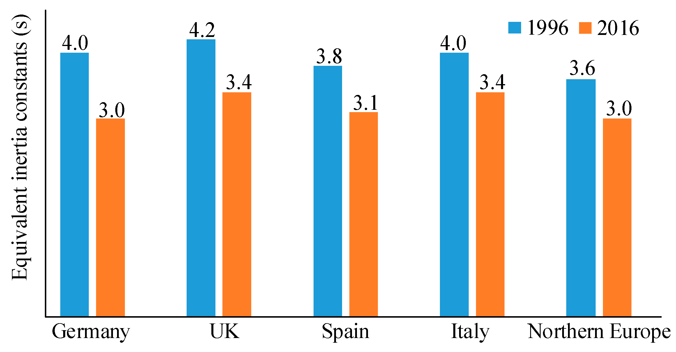
The current power system has been through transitions in intrinsic properties, one of which is represented by the decreasing of the overall inertia. The inertia is an important indicator to evaluate the strength of the power systems because inertial response (IR) can slow down the rate of change of frequency (ROCOF) and buy time for the activation of primary frequency response (PFR) to reduce nadir/peak frequency (maximum frequency deviation) [6]. In order to tackle the loss of inertia in the inverter-based generation (IBG), the concept of the virtual synchronous generator (VSG) has been proposed [7,8,9,10,11,12,13]. As the control strategies of the voltage-sourced inverters (VSIs) are commonly composed of a highly programmable supplementary controller and a double-loop controller in a cascade structure, by the implementation of the VSG algorithm, the PEI external characteristics can mimic those of synchronous generators (SGs) closely [9]. Therefore, the well-developed theory for the operation of the SG-based power system can still be exploited for the evolving power grids [7]. Two classical models, the ‘synchronverter’ and Ise’s, focus on the loss of inertia in conventional VSI droop control, and the emulation of the properties of the inertia and the speed-governor is implemented [9,11,13]. Experiment-based studies can be found in [14,15] for stand-alone applications. In [12], the equivalence between the VSG and the frequency-droop algorithms are demonstrated. It is accurate for an individual unit, but when the VSG algorithm is implemented in the power systems, the damping coefficient of loads (which is typically 1-1.5) should be considered because it is much larger than that of the damper windings (such as 0.1) [16]. However, the above studies are all restrained in the stages of the short-term frequency response. The frequency control of the conventional power systems includes a hierarchical structure because the system operation requires the ability to respond to change in demand and supply in multiple temporal stages [17]. With higher penetration of renewable generation, the IBG units would eventually and inevitably take the responsibility of regulating the overall energy balance because of the consequent displacement of traditional SGs. Therefore, the flexibility of the power system operation requires the VSG algorithm to extend its application scope.

As the parameters of PEIs are tunable rather than restrained by physical equipment, VSG algorithms can modify the inertia properties of the renewable units in real-time. General analysis for dynamic performance can also be found in [18,19], in which the influence of inertia and droop properties are analyzed based on transfer functions. Continuous change and step change of virtual inertia parameters are designed to minimize frequency deviation and energy support [20,21,22]. The change of inertia is straightforward but arbitrary. In [10], the requirements for dynamic support are illustrated based on system operation, including the standards of the frequency nadir, the maximum ROCOF, and the duration of delivery. However, it lacks the discussion on how to quantitatively tune the parameters to satisfy these standards. In [12], a step-by-step parameter design for virtual synchronous generators is conducted based on small-signal modeling, which focuses on independent decoupling and tuning of active and reactive power loops of a single grid-connected inverter. However, this approach is oriented for coping with unbalanced grid voltages, but not for quantitative performance indices. Also, the decoupling condition includes that the short-circuit ratio is no less than 10, which is typically not satisfied in power systems [23]. In [24], quantitative performance analysis is completed for the inertial response provided by the capacitor in the DC link. However, the capacitor can only provide frequency support as an energy buffer, and the response ability is restrained by the predesigned capacitance. Again, from the view of the operation flexibility, the quantitative performance analysis for the overall power systems should be considered for the generation mix (SGs and IBG units).

Within a microgrid, based on the information technology and communication network, secondary frequency regulation (SFR) and tertiary frequency regulation (TFR) could also be implemented on VSIs [25,26,27,28,29]. In recent research, the VSG-based IBG can also participate in system frequency regulation when active power reserves (APRs) are implemented. Instead of the traditional maximum power point (MPP) tracking, the APR strategy controls the IBG units to operate at a sub-optimal point [30]. Therefore, generation availability is reserved to tackle the power imbalance caused by the uncertain nature of renewables [31]. Active power reserves by RG units can be realized by two types of control strategies: (1) the delta control, which deloads RG units by constant percentages or values, or both according to the meteorological conditions [32]; and (2) the balance control, which controls the RG output by upper limit when the surplus power acts as reserves [33]. The APR control strategy enables the IBG units with persistent generation availability to participate not only short-term frequency response stages (IR and PFR) but also long-term frequency regulation stages (SFR and TFR). Therefore, a complete hierarchical structure of multiple temporal frequency control stages could be emulated on the VSG-based IBG units.

In order to enhance the VSG algorithm to sustain the flexibility level of power systems containing a mixed generation at all times, in this paper, a quantitative approach of performance tuning for VSG-PEIs participating in multiple temporal stages of frequency control is presented. The contributions of this work could be summarized as follows:

(1) Besides the capabilities of IR and PFR, by referring to the knowledge of conventional generation and operation, an enhanced control strategy for the capabilities of SFR and TFR are designed to complement the VSG algorithm. Therefore, VSG-based PEIs could perform multiple temporal frequency control.

(2) The analysis of frequency response dynamics, based on the simplification of the transfer function down to the second-order form, is conducted for both the stages of (1) IR and PFR, and (2) SFR. Six performance indices are proposed, and the frequency responses influenced by different parameters are analyzed.

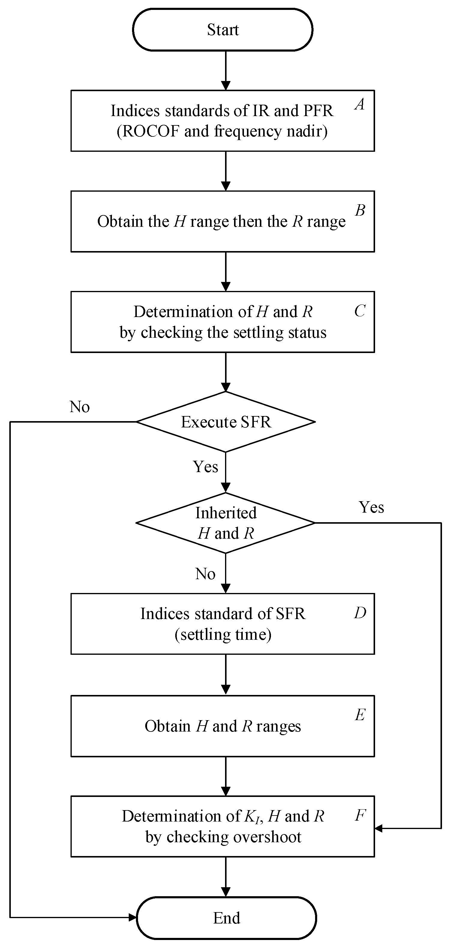
(3) It is noted that the performance indices are influenced by composite parameters, but the hierarchical stages of IR, PFR, and SFR operate in chronological order. Therefore, a parameter tuning algorithm is designed in which the parameters are also determined following a chronological sequence.

(4) The proposed parameter tuning approach could either be used to analyze dynamic performance and tune parameters for either the bulk system performance after the power unbalance disturbances or the dominant generation units in a stand-alone scenario.

The rest of the paper is organized as follows: Section 2 presents the complete emulation control strategies for PEIs with multiple temporal frequency control. Section 3 analyzes the parameter influence on the IR and PFR stages. Section 4 analyzes the parameter influence on the SFR stage. Through analyzing the composite influence on system performances by different parameters, Section 5 proposes a parameter tuning algorithm by consideration of the time sequence of performance indices in the multiple frequency control stages. Section 6 verifies the proposed algorithm by simulation.

2. VSG Emulation Control Strategies for VSIs with Frequency Control

For the IBG, the external characteristics are largely determined by the supplementary controller in the control structure. In inchoate studies, among the VSG implementations in different orders, the simplest second-order model is with better stability in transients [34] and can be combined with virtually any VSI control strategies involving a cascade structure [35]. By the implementation of the VSG algorithm, the IBG is capable of performing IR and PFR in the same way as the SGs.

The equations of motion, describing the effect of unbalance between the mechanical torque and the electromagnetic torque on rotation, could be found in many classical textbooks (such as [16]). The inertial response of the SGs is instantaneous without prerequisite measurements. For traditional SGs, the inertia is provided by the kinetic energy stored in the rotation equipment. The inertia constant H_SG indicates the inertia property, which can be expressed as

$$H_{SG}=\frac{J_{SG}{\omega }_r^2}{2{VA}_{base}}$$

(1)

where J is the moment of inertia, ${\omega }_r$ is the angular speed of the rotor, VA_base is the rated power. Similar to H_SG, the virtual inertia constant H_vir of PEIs can be analogically expressed as the ratio of the provided energy to its rated power

$$H_{vir}=\frac{J_{vir}{\omega }_m^2}{2{VA}_{base}}$$

(2)

where J_vir is the virtual moment of inertia, ${\omega }_m^{}$ is the virtual angular speed. The inertial response follows Newton’s law of motion which can be expressed as the swing equation,

$$P_m-P_e=\frac{d\Delta {\omega }_r/dt}{2H_{SG}}+D\Delta {\omega }_r$$

(3)

where D is the damping coefficient of frequency sensitive load, P_m and P_e are the virtual mechanical and electrical power (when the initial status is assumed as 0, and the second-order terms are neglected), ${\omega }_r$ is virtual angular speed. When the swing equation is represented by inertia constant, all the parameters are per-unit values.

The PFR of SGs is provided by the turbine-governor system [16]. In per unit value, for a typical SG with a reheat steam turbine, the droop property is

$$\Delta Y=-\frac{1}{R}\times \frac{1}{1+s{T}_G}\times \frac{1+s{F}_{HP}{T}_{RH}}{(1+s{T}_{CH})(1+s{T}_{RH})}\Delta {\omega }_r$$

(4)

where R is the speed droop, Y is the valve position, T_G is the time constant of speed governor, and F_HP, T_RH, T_CH are typical parameters for a reheat steam turbine. The emulation for the properties of turbine-speed governor systems of SGs is necessary when the VSG-based PEIs are operated in parallel with traditional power plants.

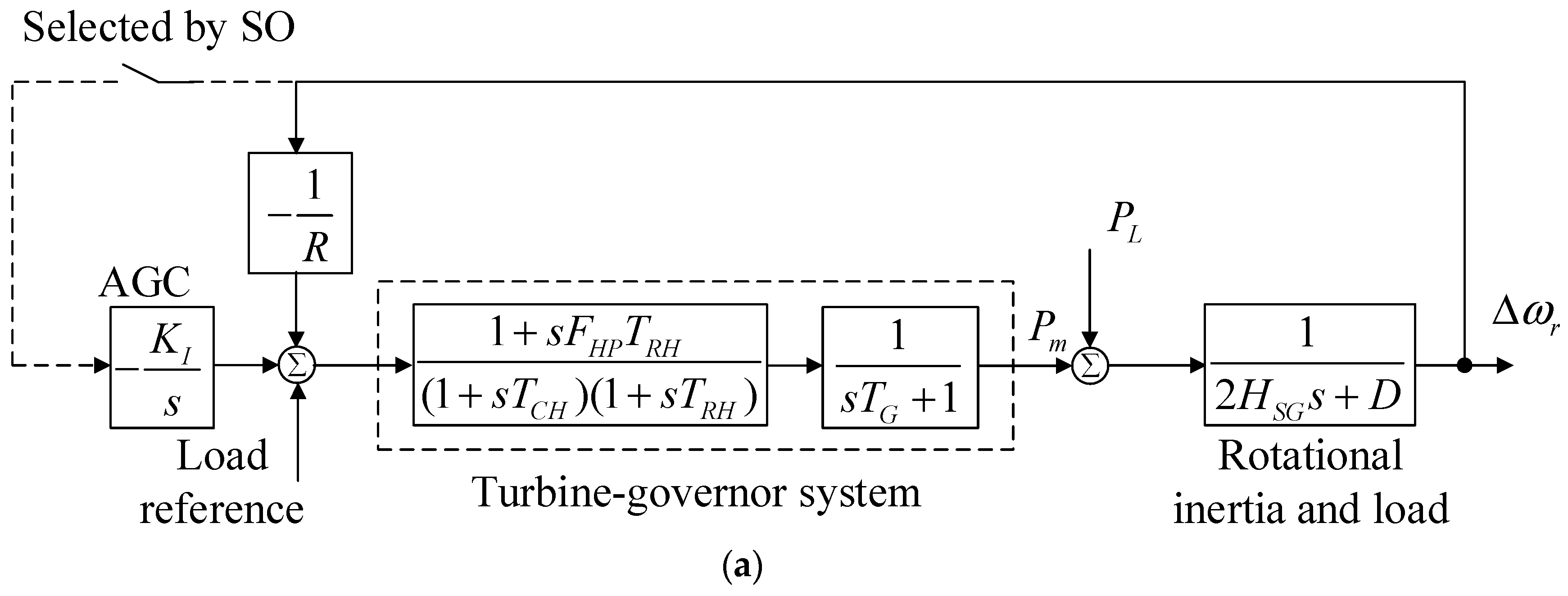
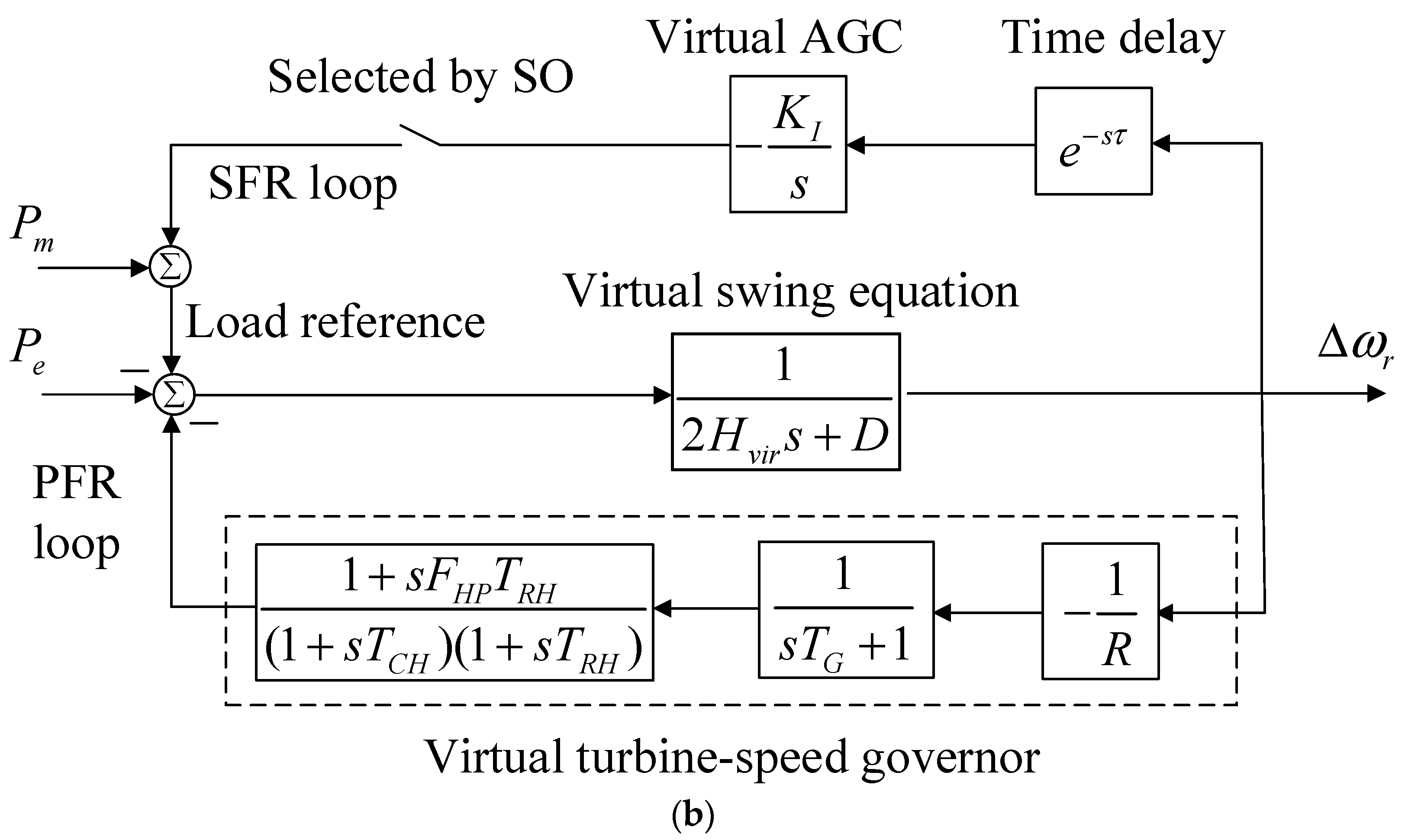
By the exploitation of conventional theories of the SG-based power system, the VSG algorithm also enables the PEIs to perform SFR and TFR. The SFR kicks in when the frequency deviation lasts for a preset time period after the frequency is stabilized by the IR and PFR. The TFR is activated by the system operator (SO) to set the load reference for each generation unit. For traditional SGs, the SFR and TFR are executed by the regulation of load reference settings, which is shown in Figure 1a. The variables of load references also pass through the blocks of the turbine-governor system. However, because only specific units in the power system are selected to perform automatic generation control (AGC) regulation, when the emulation of AGC is implemented on VSG-PEIs, the load reference can be directly fed into the block of the virtual swing equation, as shown in Figure 1b. In Figure 1b, $\tau$ is the time delay of SFR, K_I is the coefficients of the integral controller.

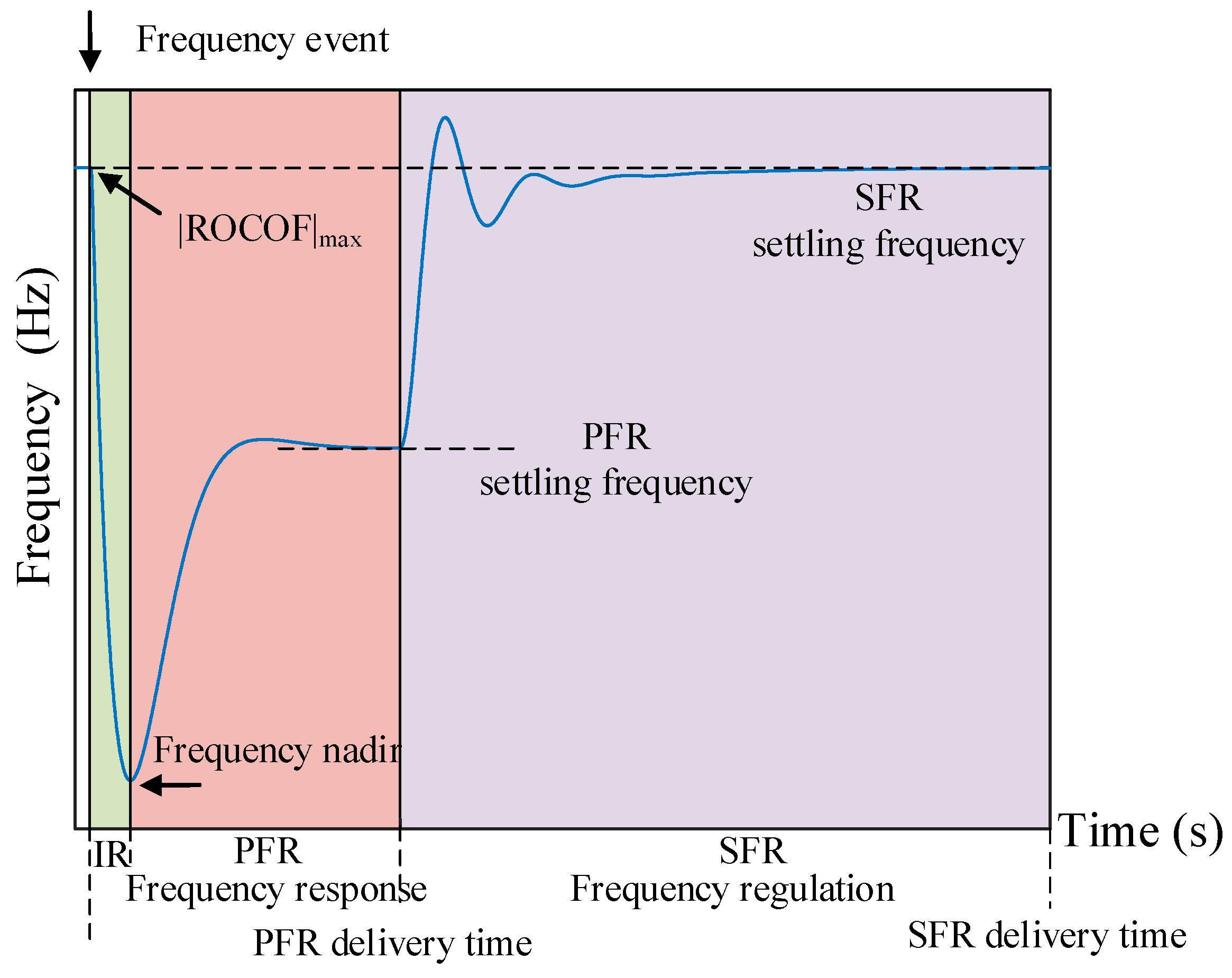
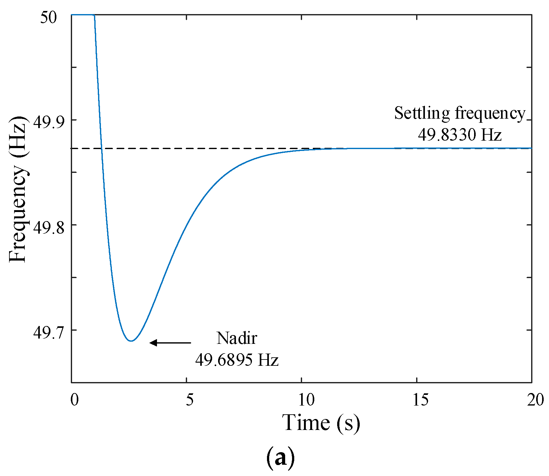
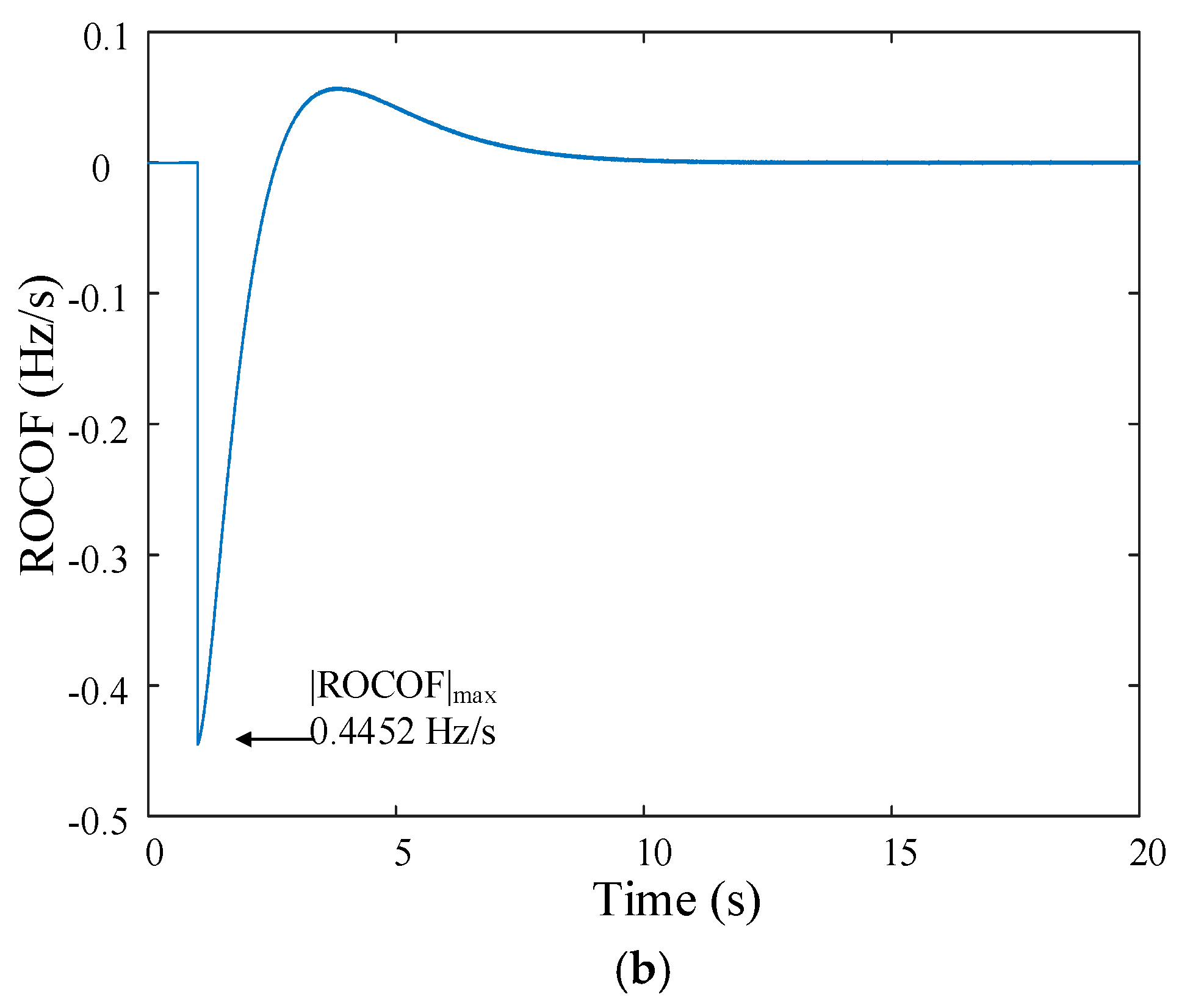
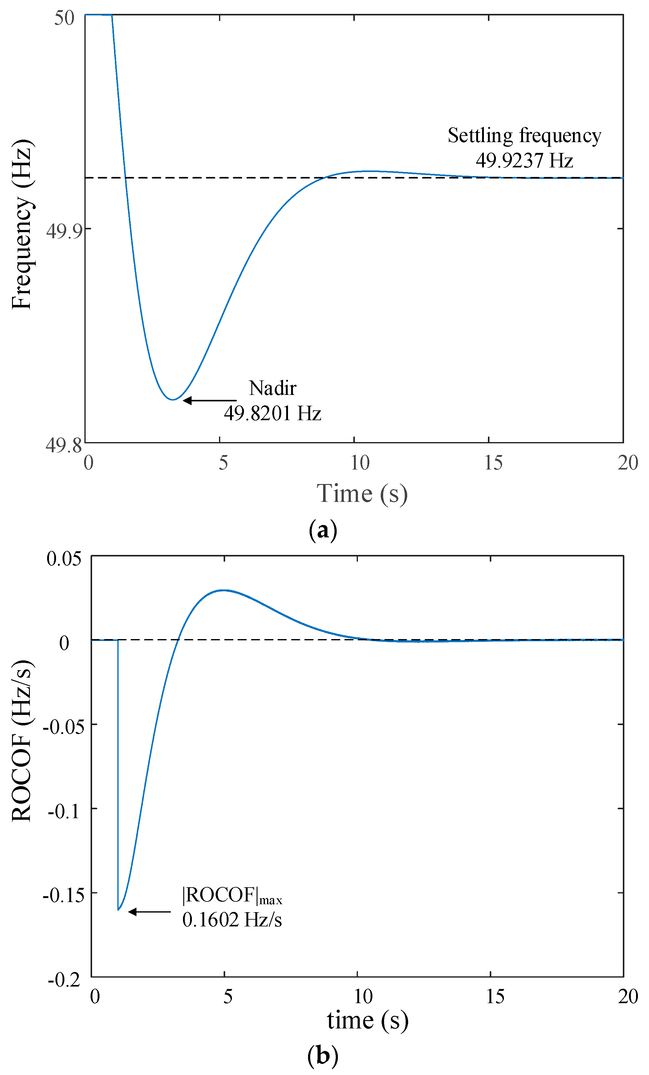
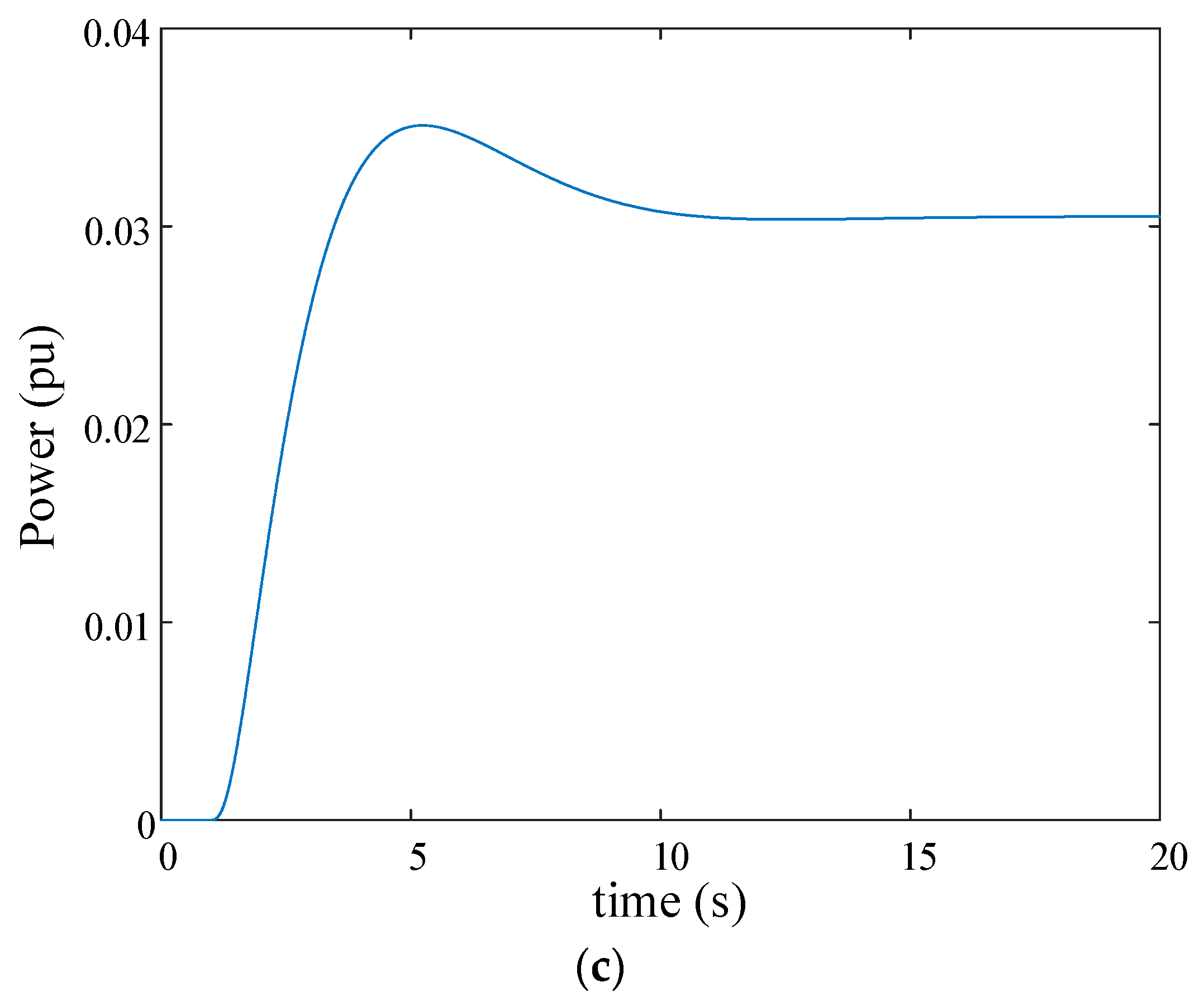
The system frequency indicates the overall power balance between the generation and the demand at any instantaneous time. In the traditional SG-dominated power system, active power-frequency control is a series of multiple temporal processes that can be divided into four stages [16]. As the VSG algorithm can fully emulate the frequency control performance of the SGs, the multiple temporal frequency control is also provided by the VSG-PEIs. For quantitative analysis, the performance indices mainly include the maximum ROCOF, the frequency nadir, the settling frequency, and the settling time, which are shown in Figure 2.

Furthermore, in a small synchronous area, the equivalent inertia constant $H_{sys}$ of different VSG-based PEIs and SGs can be expressed as

$$H_{sys}={\displaystyle \sum _{i=1}^n(H_i\frac{S_i}{S_{sys}}})$$

(5)

where n is the total number of generation units with inertia properties, $H_i$ and $S_i$ are the inertia constant and power rating of the i-th unit, respectively, $S_{sys}$ is the power base of the system [32,36]. Also, the equivalent speed droop $R_{eq}$ can be expressed as

$$R_{eq}=\frac{1}{{\displaystyle \sum _{i=1}^n\frac{1}{R_i}}}$$

(6)

where $R_i$ is the speed droop property of the i-th generation unit [16].

Consequently, for a local synchronous system, the generation units can be simplified and equivalent to a single unit. The emulation strategy mentioned before could be considered as the overall characteristics of the entire local synchronous area. Then once the parameters are tuned, it could either be used to control the dominated PEI in a stand-alone system or calculate the parameters reversely for individual units with inertia properties.

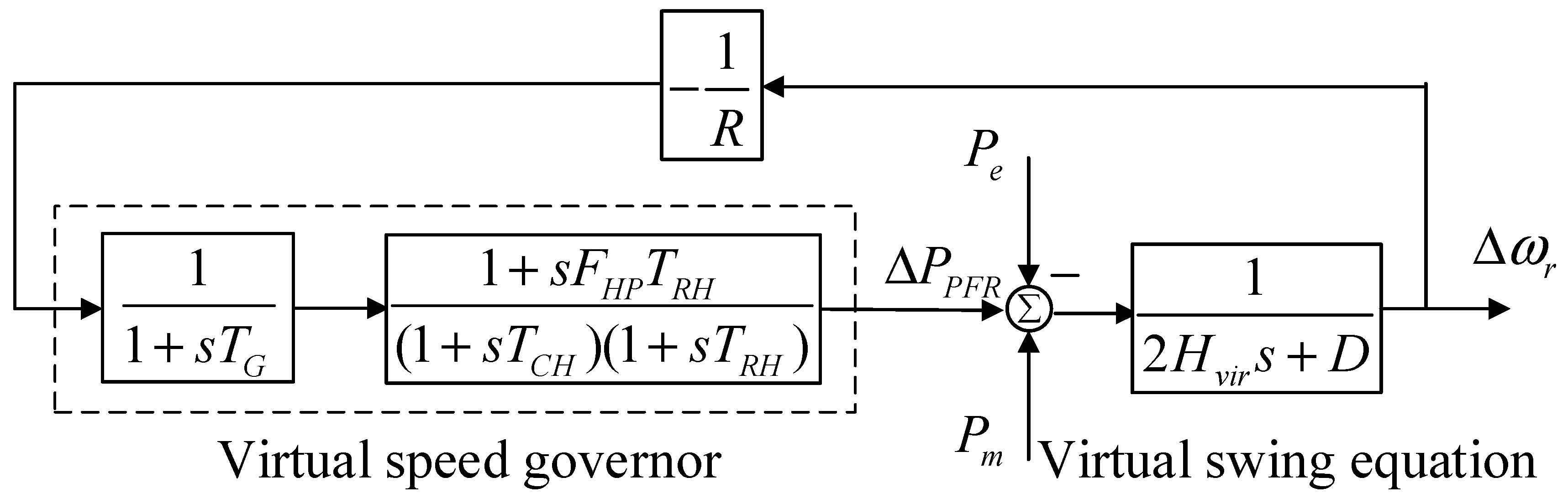
3. Simplification of the Dynamic System in IR and PFR Stages

The emulation of IR and PFR is derived from the mechanism imitation of the swing equation and the turbine-speed governor system. The effect of the closed-loop transfer function of the VSI based on the cascade control structure is assumed to be fast and accurate. Then the high-order system involving virtual IR and PFR can be simplified into a second-order dynamic system by the dominant poles and zeros without too much error. The performance indices can be deduced from the simplified transfer function. Take a stand-alone VSG-PEI supplying isolated load for example, the block diagram involving IR and PFR is shown in Figure 3.

For a step change of demand $\Delta P_L$, the transfer function from $\Delta P_L$ to the virtual angular speed of rotor $\Delta {\omega }_r$ is

$$G(s)=\frac{\Delta {\omega }_r}{\Delta P_L}=\frac{-R(1+s{T}_G)(1+s{T}_{CH})(1+s{T}_{RH})}{(2Hs+D)(1+s{T}_G)(1+s{T}_{CH})(1+s{T}_{RH})R+s{F}_{HP}{T}_{RH}+1}$$

(7)

For SGs with reheat steam turbines, typical parameters are shown in

Table 1. Typical parameters of an SG with a reheat steam turbine [16].

Parameter	Value	Unit	Parameter	Value	Unit
R	0.05	pu	FHP	0.3	pu
H	5	pu	TRH	7	s
D	1	pu	TCH	0.3	s
TG	0.2	s

.

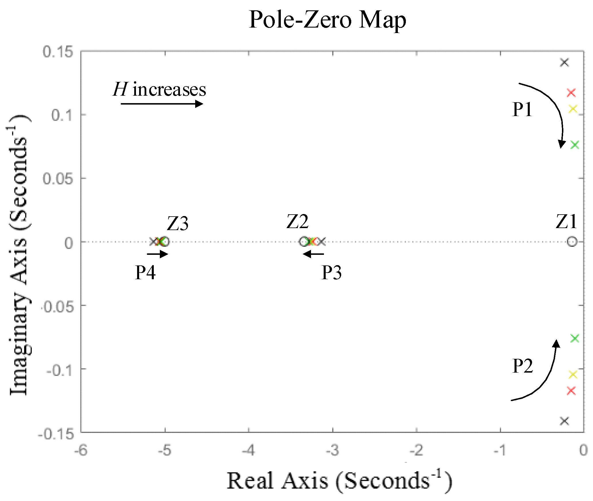
The pole-zero map of the transfer function is shown in Figure 4. From the transfer function G(s), the zeros are fixed on the real axis. With the increasing of H, the poles P3 and P4 tend to approach the zeros Z2 and Z3. As P3 and P4 are fast poles and very close to Z2 and Z3, the dynamic responses are mainly determined by the dominant zeros Z1 and the slow poles P1 and P2 [37]. It is noted that the inertia constants of different SGs, which are shown in

Table 2. Typical inertia constant of traditional synchronous machines [16].

Type of Generation Unit		Inertia Constant
Thermal unit	(1) 2 poles	2.5–6.0
	(2) 4 poles	4.0–10.0
Hydraulic unit		2.0–4.0

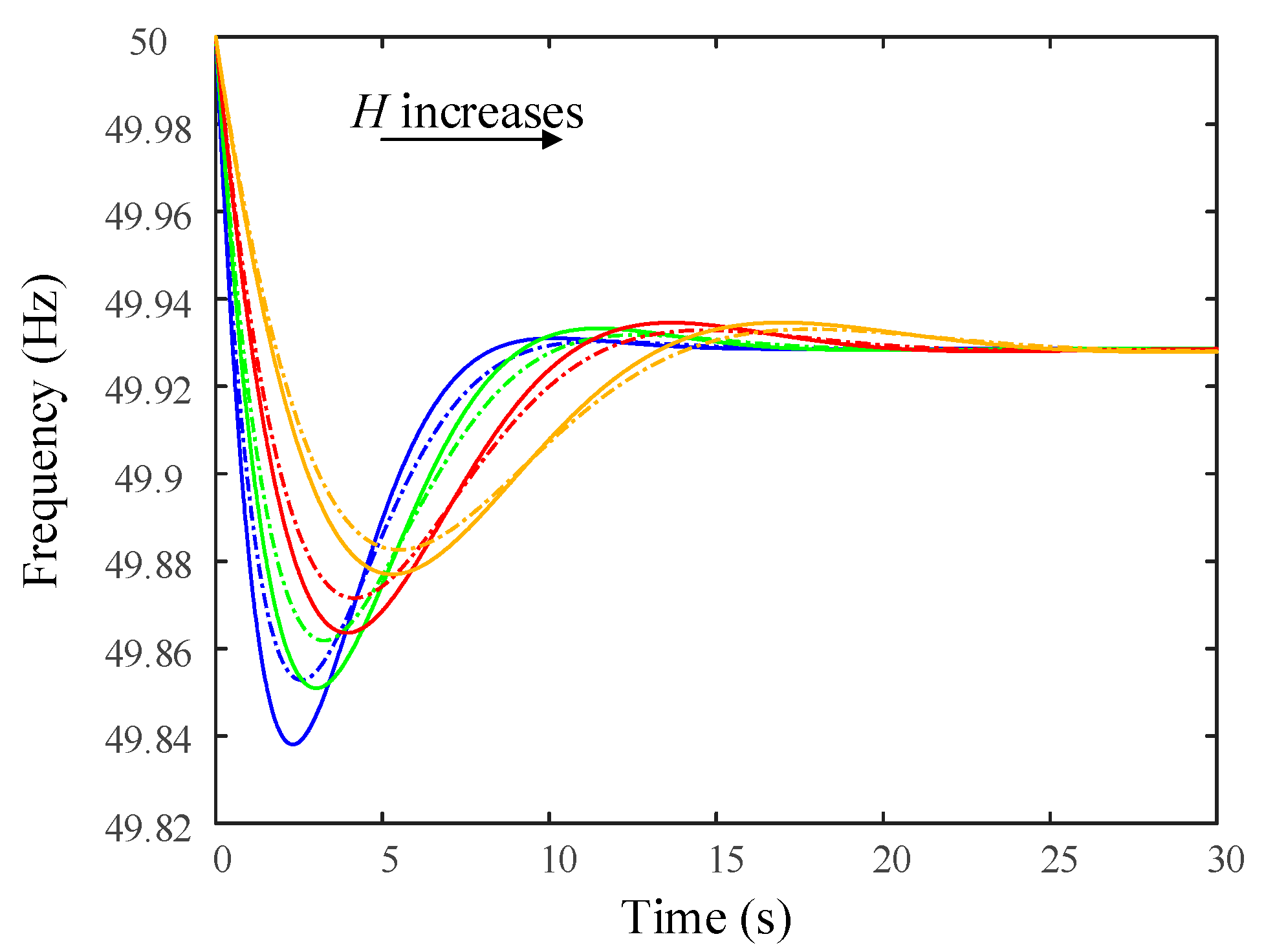
, are in a small range rather than accurately the same [16]. The concept of VSG is to enable the PEIs to provide approximately synchronous responses like traditional SGs. Moreover, fast poles influence the early part of the time history [37]. The frequency responses based on the transfer function of the original and simplified systems are shown in Figure 5, which shows the maximum error between the two dynamic systems is less than 10% frequency deviation. Therefore, the estimation by the dominant zeros and poles are practically acceptable.

According to the dominant zeros and poles (Z1, P1, and P2), the simplified transfer function of the dynamic system is derived from Equation (7), which can be expressed as

$$\begin{array}{cc}\hfill G(s)& =\frac{-R(1+s{T}_{RH})}{(2Hs+D)(1+s{T}_{RH})R+s{F}_{HP}{T}_{RH}+1}\hfill \\ & =K\frac{s+z_1}{s^2+2\zeta {\omega }_{n}s+{\omega }_n^2}\hfill \end{array}$$

(8)

where ${\omega }_n$ and $\zeta$ are the undamped natural frequency and damping ratio [37],

$$\begin{array}{c}K=-\frac{1}{2H},z_1=\frac{1}{T_{RH}},{\omega }_n=\sqrt{\frac{1+RD}{2HR{T}_{RH}}}\hfill \\ \zeta =\frac{2HR+T_{RH}DR+F_{HP}{T}_{RH}}{4HR{T}_{RH}}\times \sqrt{\frac{2HR{T}_{RH}}{1+RD}}\hfill \end{array}$$

(9)

When the system is subjected to a step increase in demand

$$\Delta P_L=\frac{\Delta p}{s}$$

(10)

By multiplying (8) and (10) and taking the inverse Laplace transformation, the dynamic response of frequency deviation in time-domain can be expressed as

$$\Delta f(t)=K\Delta p\times [\frac{z_1}{{\omega }_n^2}+A{e}^{-\zeta {\omega }_{n}t}\sin ({\omega }_{d}t+\beta )]$$

(11)

where

$$\begin{array}{c}{\omega }_d={\omega }_n\sqrt{1-{\zeta }^2}\hfill \\ A=\sqrt{{(\frac{z_1\zeta -{\omega }_n}{{\omega }_d{\omega }_n})}^2+{(\frac{z_1}{{{\omega }_n}^2})}^2}\hfill \\ \beta =\arctan [\frac{z_1{\omega }_d}{{\omega }_n(z_1\zeta -{\omega }_n)}]+\pi \hfill \end{array}$$

(12)

Assuming the original state of the frequency is 1.0 pu, the frequency response is

$$f(t)=1+K\Delta p\times [\frac{z_1}{{\omega }_n^2}+A{e}^{-\zeta {\omega }_{n}t}\sin ({\omega }_{d}t+\beta )]$$

(13)

From Equation (11), performance indices during IR and PFR can be derived. First, the rate of change of frequency (ROCOF) is

$$\begin{array}{cc}\hfill ROCOF=& \frac{d\Delta f}{dt}-K\Delta p\times [A\zeta {\omega }_n{e}^{-\zeta {\omega }_{n}t}\sin ({\omega }_{d}t+\beta )-\hfill \\ & A{\omega }_d{e}^{-\zeta {\omega }_{n}t}\cos ({\omega }_{d}t+\beta )]\hfill \end{array}$$

(14)

It is noted that, when t = 0, ROCOF reaches maximum magnitude, which can be expressed as

$${ROCOF}_{\max }=-K\Delta p\times (A\zeta {\omega }_n\sin \beta -A{\omega }_d\cos \beta )$$

(15)

From Equation (11), when ROCOF = 0, the peak time $t_{peak}$ (the time when the frequency reaches a nadir or a peak) can be expressed as

$$t_{peak}=\frac{1}{{\omega }_d}(\arctan \frac{\sqrt{1-{\zeta }^2}}{\zeta }-\beta )$$

(16)

Substitute (16) to (13), then the peak frequency f_peak (or nadir) is

$$f_{peak}=1+K\Delta p\times \frac{z_1}{{\omega }_n^2}+K\Delta pA{e}^{-\zeta {\omega }_n{t}_{peak}}\sqrt{1-{\zeta }^2}$$

(17)

When the third item in the Equation (17) decays approximately to zero, the quasi-steady-state frequency f_ss is achieved, which can be expressed as

$$f_{ss}=1+K\Delta p\times \frac{z_1}{{\omega }_n^2}=1-\frac{R}{DR+1}\Delta p$$

(18)

The frequency deviation can also be evaluated by the frequency overshoot $\sigma$, which can be expressed as

$$\sigma =\left|\frac{f_{ss}-f_{peak}}{f_{ss}}\right|\times 100\%=\left|\frac{A{\omega }_n^2\sqrt{1-{\zeta }^2}{e}^{-\zeta {\omega }_n{t}_{peak}}}{z_1+{\omega }_n^2/K\Delta p}\right|$$

(19)

The settling time t_s can be defined as the dynamic response enters the 2% quasi-steady-state error band [17],

$$\left|\frac{f(t_s)-f_{ss}}{1-f_{ss}}\right|=2\%$$

(20)

and by submitting Equations (11) and (12) into Equation (20), the settling time can be deduced as

$$t_s=-\frac{1}{\zeta {\omega }_n}\ln \frac{z_1}{50A{\omega }_n^2}$$

(21)

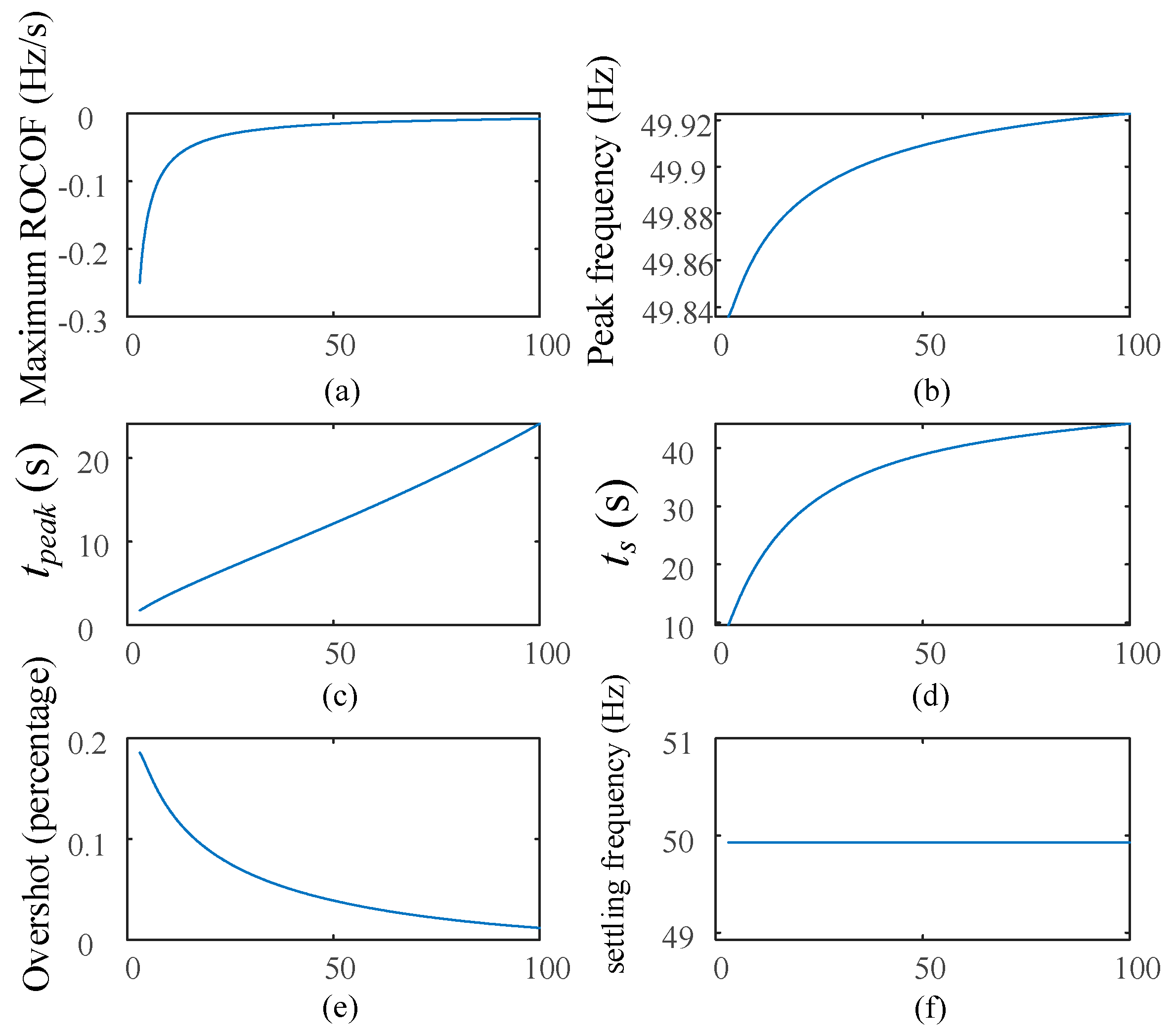
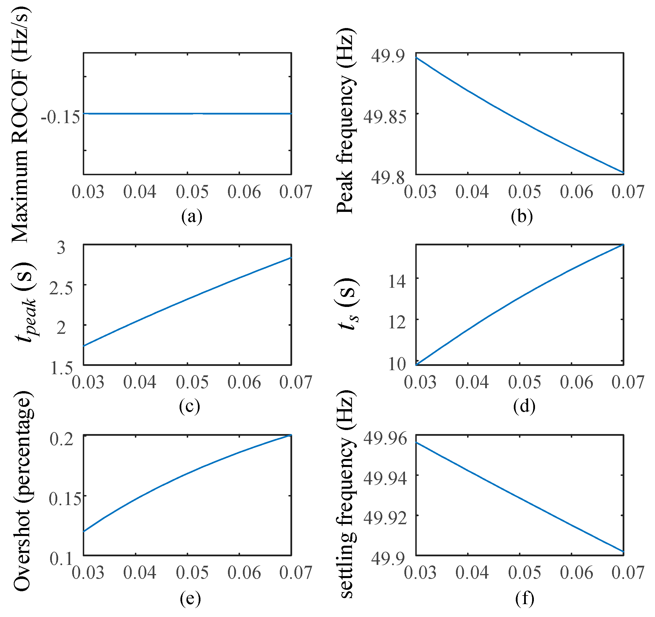
From the performance indices, the effect of separate parameters on system performance can be derived. When subjected to a step increase of load by 0.03 pu, the trends of the above performance indices corresponding to different H and R are shown in Figure 6 and Figure 7. In Figure 6, R is set as a constant, and in Figure 7, H is set as a constant.

From Figure 6a,b,e, the increasing of inertia constant H leads to the decreasing of the magnitude of ROCOF, frequency nadir, and the overshoot. Therefore, it proves that inertia property could suppress the ROCOF and improve frequency nadir. From (c), the increasing of H also delays the peak time. However, the increasing H would slow down the dynamic responses, which is shown in (d). Therefore, there is a trade-off between the nadir improvement and the delivery time. From (f), the settling frequency is irrelative to H.

From Figure 7a, percentage R does not influence the ROCOF. From (b) and (e), the nadir gets worse, and the overshoot increases as the percentage R increases. From (c) and (d), the changes in percentage R do not alter the peak time and settling time very much. From (f), the increase of R would decrease the settling frequency. Consequently, the speed droop coefficient R indicates the proportional relationship between the amount of support power and the counteracted frequency deviation. The lower R represents a larger amount of active power supported, which results in a better nadir.

4. Simplification of the Dynamic System in SFR Stages

The secondary control regulates the reference generation output and restores the system frequency to the nominal. The SFR is activated after the PFR has stabilized the system frequency. In VSG-PEI, the virtual SFR is executed by adding an integrator, shown in Figure 1b. After the frequency is stabilized, when the SFR kicks in, the transfer function of the dynamic system in the new stage is

$$\begin{array}{cc}\hfill G(s)=& (-R(1+s{T}_G)(1+s{T}_{CH})(1+s{T}_{RH})s)/\hfill \\ & (s(1+s{F}_{HP}{T}_{RH})+K_{I}R(1+s{T}_G)(1+s{T}_{CH})(1+s{T}_{RH})+\hfill \\ & (2Hs+D)(1+s{T}_G)(1+s{T}_{CH})(1+s{T}_{RH})Rs)\hfill \end{array}$$

(22)

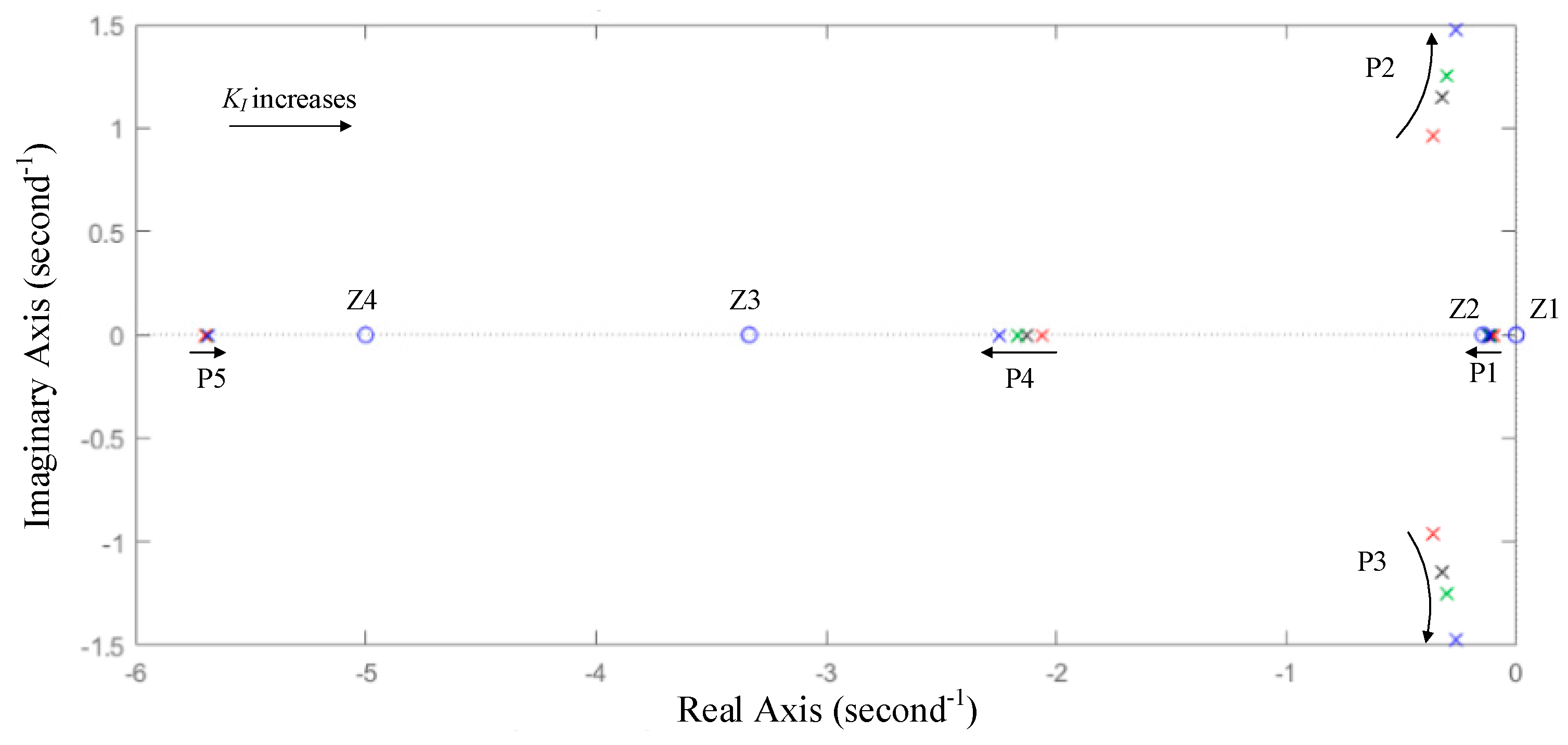
The pole-zero map of the transfer function is shown in Figure 8.

From the pole-zero map, the zeros are fixed on the real axis. With the increasing of K_I, P1 tends to approach to Z2, which results in the mutual cancelation of effects. The effect of poles P4 and P5, and the zeros Z3 and Z4, which are far away from the imaginary axis, would be neglected for simplifications. Therefore, the poles P2 and P3, and the zero Z1 are dominant in the dynamic processes.

From the slow zeros and poles (Z1, P1, and P2), the system transfer function (Equation (22)) is simplified into the second-order, which can be expressed as

$$G(s)=\frac{-Rs}{s(1+s{F}_{HP}{T}_{RH})+K_{I}R+R(Ms+D)s}=K\frac{s+z_1}{s^2+2\zeta {\omega }_{n}s+{\omega }_n^2}$$

(23)

where ${\omega }_n$ and $\zeta$ are the undamped natural frequency and damping ratio,

$$\begin{array}{c}K=-\frac{R}{F_{HP}{T}_{RH}+MR},z_1=0,{\omega }_n=\sqrt{\frac{K_{I}R}{F_{HP}{T}_{RH}+MR}}\hfill \\ \zeta =\frac{DR+1}{2(F_{HP}{T}_{RH}+MR)}\times \sqrt{\frac{F_{HP}{T}_{RH}+MR}{K_{I}R}}\hfill \end{array}$$

(24)

It is noted that the initial status in the dynamic system is inherited from the IR and PFR stages. By taking the inverse Laplace transformation, the dynamic response of system frequency in time-domain is derived, which can be expressed as

$$f(t)=1-\frac{K}{{\omega }_d}{e}^{-\zeta {\omega }_{n}t}\sin {\omega }_{d}t$$

(25)

where

$${\omega }_d={\omega }_n\sqrt{1-{\zeta }^2}$$

(26)

From Equation (25), system performance indices during SFR can be derived. First, the rate of change of frequency (ROCOF) can be expressed as

$$ROCOF=\frac{df}{dt}=-\frac{K}{{\omega }_d}\times (-\zeta {\omega }_n{e}^{-\zeta {\omega }_{n}t}\sin {\omega }_{d}t+{\omega }_d{e}^{-\zeta {\omega }_{n}t}\cos {\omega }_{d}t)$$

(27)

In Equation (27), when t = 0, ROCOF reaches the maximum value, which can be expressed as

$${ROCOF}_{\max }=-K$$

(28)

The peak time $t_{peak}$ is achieved when ROCOF = 0, then from Equation (27), the peak time can be expressed as

$$t_{peak}=\frac{1}{{\omega }_d}\arctan \frac{\sqrt{1-{\zeta }^2}}{\zeta }$$

(29)

By substituting (29) into (25), the peak frequency f_peak can be expressed as

$$f_{peak}=1-\frac{K}{{\omega }_d}{e}^{-\zeta {\omega }_n{t}_{peak}}\sqrt{1-{\zeta }^2}$$

(30)

From Equation (25), the quasi-steady-state frequency f_ss is

$$f_{ss}=1$$

(31)

For floating control, the frequency deviation can be evaluated by the frequency overshoot $\sigma$, which can be derived as

$$\sigma =\left|\frac{f_{ss}-f_{peak}}{f_{ss}}\right|\times 100\%=\left|\frac{K}{{\omega }_d}\sqrt{1-{\zeta }^2}{e}^{-\zeta {\omega }_n{t}_{peak}}\right|\times 100\%$$

(32)

The settling time t_s can be defined when the decaying exponential $e^{-\zeta {\omega }_{n}t}$ reaches 1% [37].

$$e^{-\zeta {\omega }_n{t}_s}=0.01$$

(33)

then from Equation (33), the settling time can be derived as

$$t_s=\frac{4.6}{\zeta {\omega }_n}$$

(34)

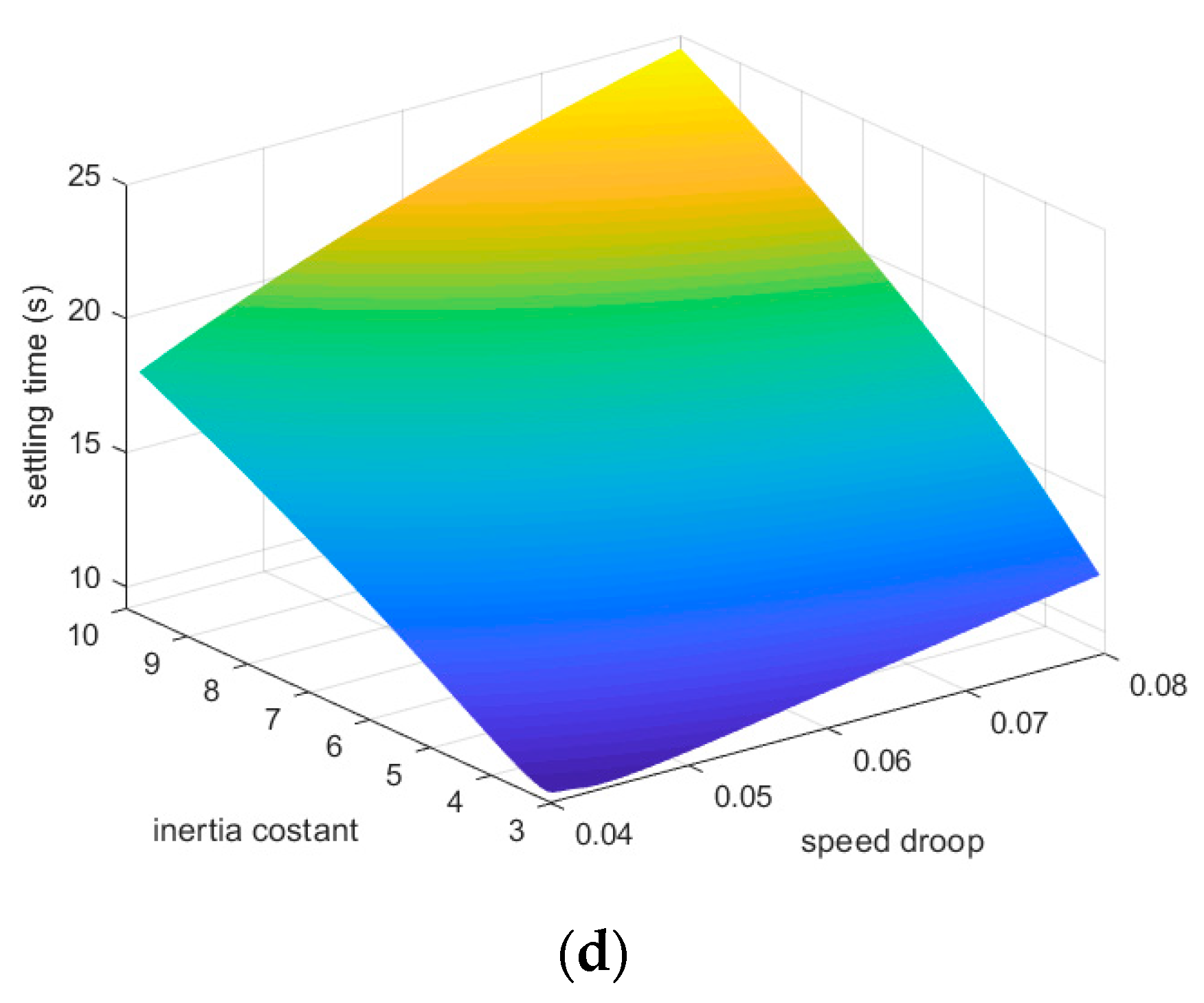
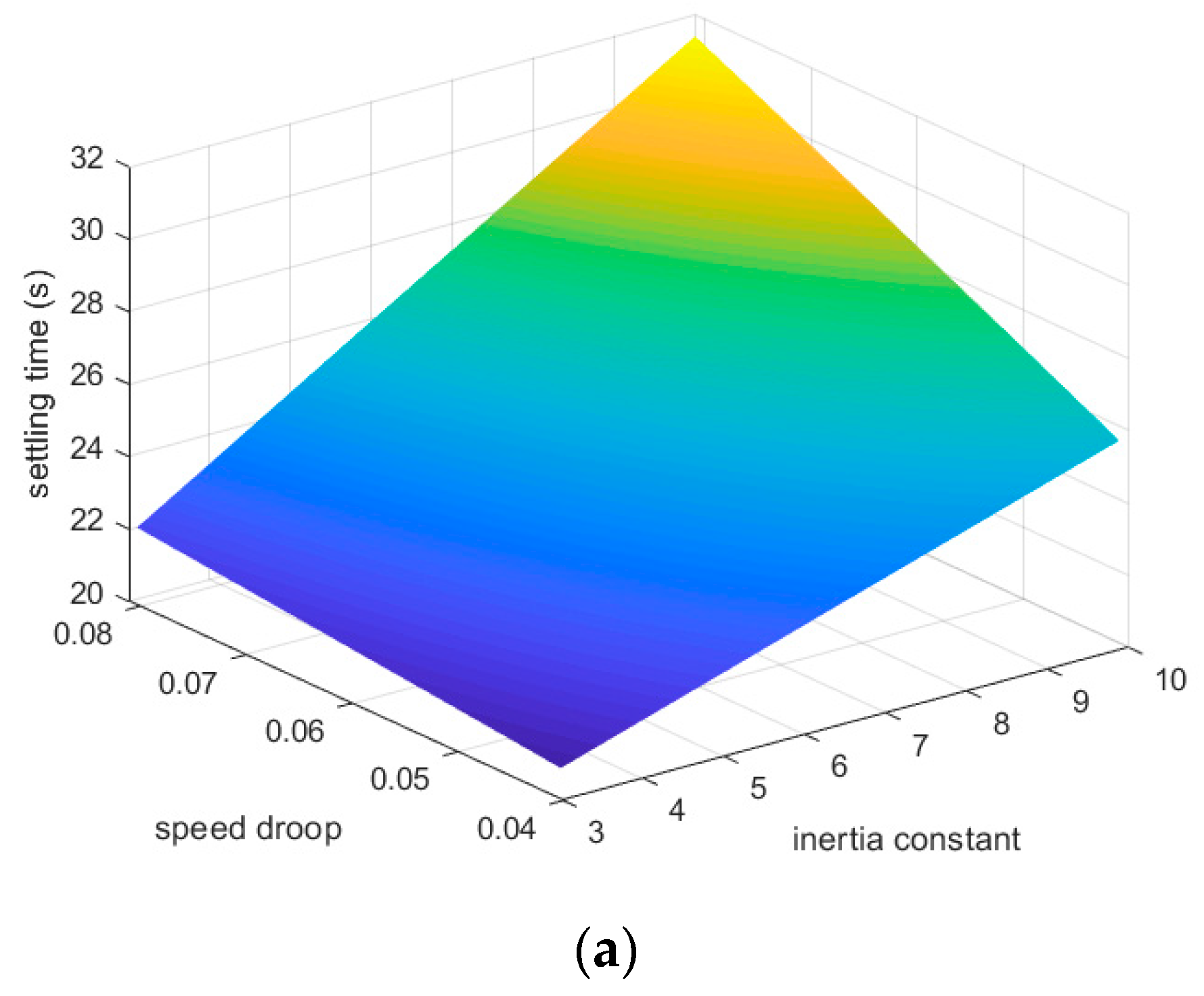
From the performance indices, the effect of separate parameters on system performance in the SFR stage can be derived. When SFR kicks in, the trends of the above performance indices corresponding to different K_I, H, and R are shown in Figure 9, Figure 10, and Figure 11, respectively.

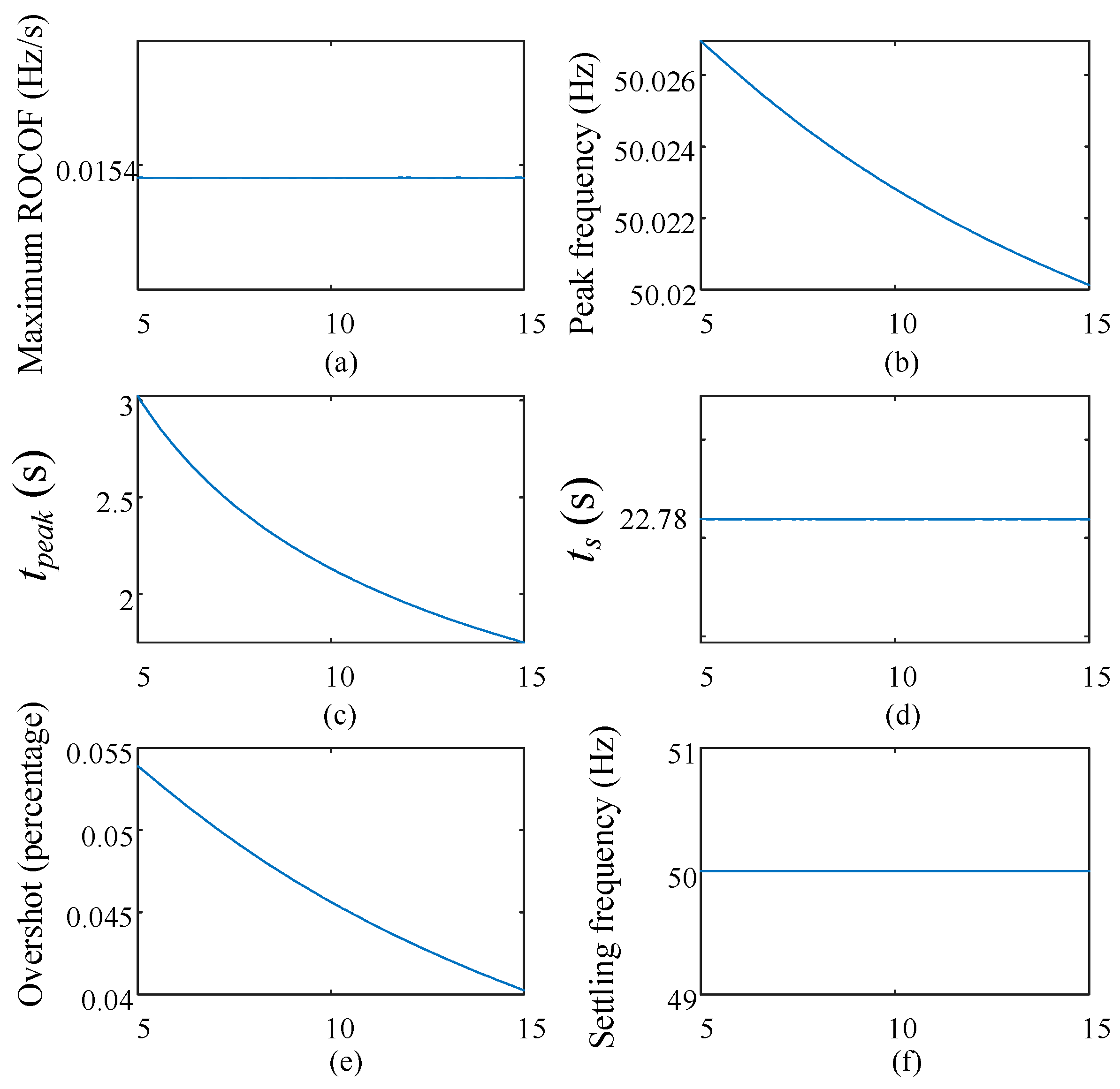
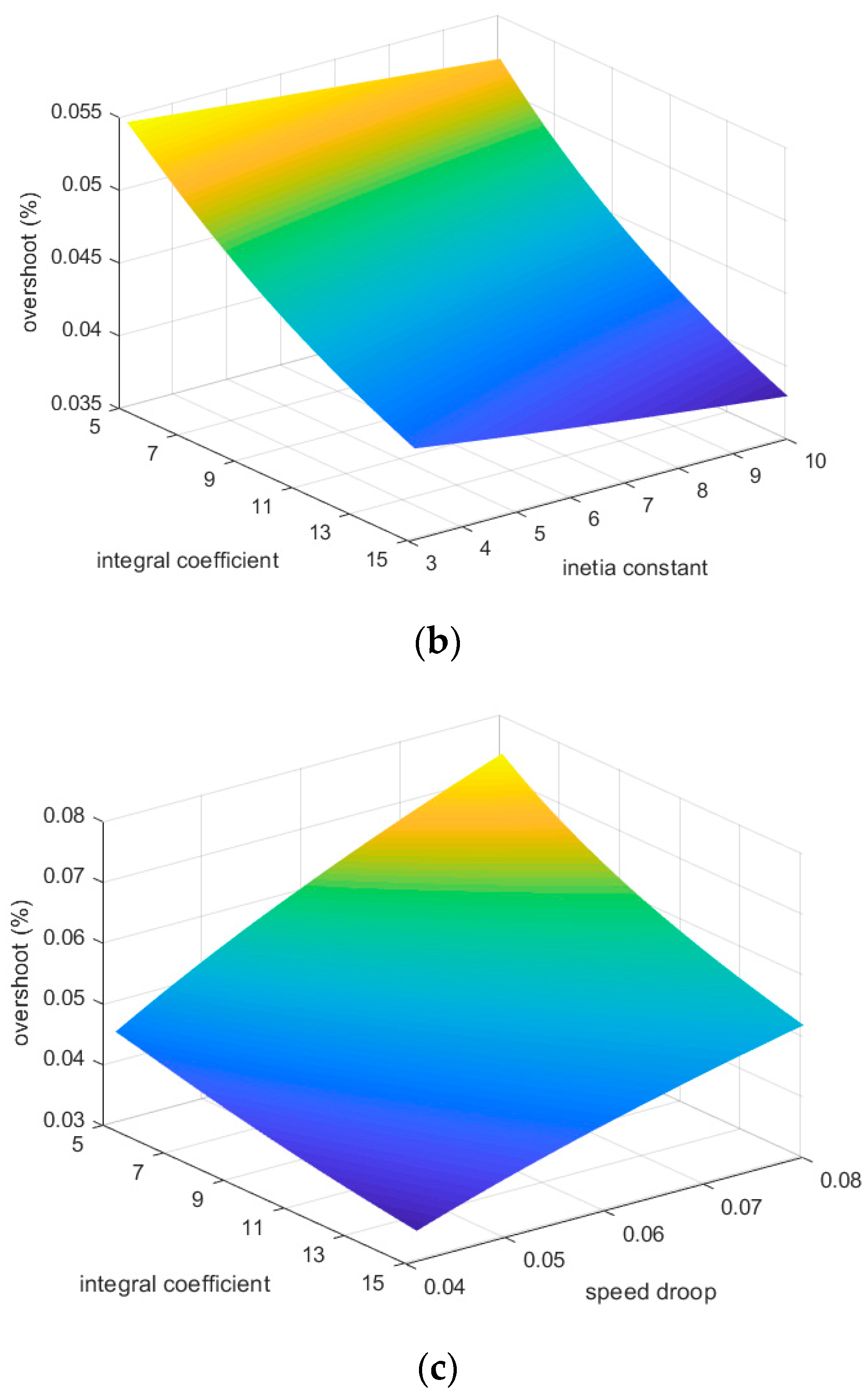
From Figure 9a,d,f, the coefficient of the integrator is irrelative to the magnitude of the ROCOF, the settling time, and the settling frequency. From (b), (c), (e), the increase of the integral effect would decrease the peak frequency, the peak time, and the overshoot.

From Figure 10a,b,e, the increasing of inertia constant would decrease the magnitude of the ROCOF, the peak frequency, and the overshoot. However, from (c) and (d), the increase of inertia property would also increase the peak time and the settling time. From (f), the inertia constant is irrelative to the settling frequency.

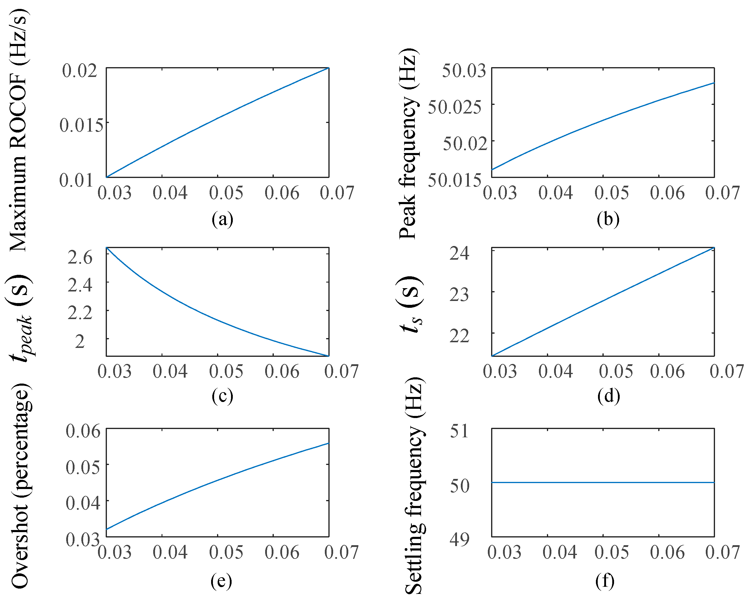
From Figure 11a,b,d,e, the increase of speed droop R would also increase the magnitude of ROCOF, the peak frequency, the settling time and the overshoot. However, from (c), the increase in speed droop would decrease the peak time. From (f), the speed droop is irrelative to the settling frequency.

5. Parameter Tuning for Frequency Response and Regulation

From the derived expressions before, the performance indices are influenced by multiple parameters. In the process of IR and PFR, the performances are determined by the composite effects of the inertia constant H and the speed droop R. In the following process of SFR, the performances are determined by the integral coefficient K_I, as well as the inherited or readjusted H and R.

5.1. Composite Parameter Analysis for IR and PFR

During the processes of IR and PFR, four key performance indices (the maximum magnitude of ROCOF, the frequency nadir, the settling frequency, and the settling time) are influenced by the composite effects of the coefficients H and R, which are shown in Figure 12. In Figure 12, H varies from 3 to 10, R varies from 0.04 to 0.08, and the step increase of load is constant.

From Figure 12, the magnitude of ROCOF decreases as H increases, but does not relate to R. The frequency nadir improves with the increase of H and the decrease of R. The settling frequency increases with the decrease of R but does not relate to H. The settling time is influenced by both H and R.

5.2. Composite Parameter Analysis for SFR

During the process of SFR, as the effect of the integration is gradual and small, two key indices, the settling time and the overshoot, are selected. The parameters in the SFR stage involve H, R, and the integral coefficient K_I. From previous results, the settling time in the SFR stage is irrelative to K_I. The overshoot is relative to all three parameters. The composite parameter influences are shown in Figure 13.

5.3. Parameter Tuning for Performance Indices

In some countries (such as Germany, the USA, and the UK), the system operators have developed a time frame for renewable penetrated grids. For example, the prescribed limit for ROCOF is 0.125 Hz/s [38]. Also, in this material, the maximum ROCOF and PFR delivery time in its case study are set to be 0.5 Hz/s and 10s, respectively. In another research, the maximum frequency deviation $\Delta f_{max}$ is set as 0.2 Hz [24]. It is noted that if the ROCOF exceeds 1 Hz/s, the frequency relay would be tripped and incur a large disturbance to a power system [39]. Generally, the delivery of PFR is required to be within 10–30s, and the time for SFR delivery is from 30 s to several minutes. The PFR capacity should always limit the frequency between 49.5–50.5Hz. The typical standards (nominal frequency is 50 Hz) are summarized in

Table 3. Performance indices for IR and PFR.

Performance Indices	Standard
Maximum ROCOF magnitude	0.125–0.5 Hz/s
Frequency nadir/peak magnitude	0.2–0.5 Hz
Settling frequency	49.5–50.5 Hz
PFR delivery time	10–30 s
SFR delivery time	30 s–minutes

.

It is noted that the stages of IR, PFR, and SFR activate in chronological order. Therefore, based on the composite effects and the standards, a flowchart of parameter design for VSG-PEIs is shown in Figure 14. In step A, the standards for ROCOF and frequency nadir are input. The maximum ROCOF only relates to inertia constant, so the range of H could be determined according to the ROCOF standard. The frequency nadir relates to both H and R, then according to the H range and the nadir requirement, the range of R could be determined. Therefore, in step B, the satisfying ranges of H and R are obtained. In step C, the desired H and R are determined by checking the settling frequency and the settling time. If the VSG-PEI does not participate in the following SFR, the design comes to an end. Otherwise, the parameter design goes on for the SFR stage. If the parameters of H and R are inherited from the previous, it jumps to step F. If not, in step D and E, the standard of settling time is input, and the satisfying ranges of H and R are obtained. In step F, K_I, and H, R are determined by checking the overshoot.

6. Case Study and Simulation

In this section, the proposed VSG emulation strategies and the parameter tuning approach are verified in simulation through MATLAB/Simulink. Based on the predetermined standards of the performance indices shown in

Table 4. Predetermined standards of performance indices.

Performance Indices	Standard
Maximum ROCOF magnitude	0.5 Hz/s
Frequency nadir/peak magnitude	0.2 Hz
PFR Delivery time	Within 20 s
SFR Delivery time	Within 40 s

, the parameters in the simulation are shown in

Table 5. Parameters in simulation.

Parameter	Value	Unit	Parameter	Value	Unit
Vdc	800	V	Heq	5	pu
Vac	0.22	kV	D	1	pu
L	10	mH	R	0.05	-
C	350	$\mu F$	Voltage droop	3%	pu
f	50	Hz	Load step	0.03	pu
fpwm	5000	Hz	Step time	1	s
VAbase	15000	W	KI	10	-
$\tau$	20	s

.

6.1. Frequency Response in the Initial Systems and Previous Approaches

From 1996–2016, the equivalent inertia constants H_eq in many European countries and districts have decreased larger than 15%, which are shown in Figure 15 [40]. Considering the worst case in which the inertia constant H_eq = 3.0, the frequency response of the system without renewable participation is shown in Figure 16. The percentage droop is set as 5.

In the previous research, renewable penetration is typically set varying from 10% to 30% [38], and the inertia constant for VSG-IBG is usually set as 5.0 s. According to Equation (5), under the worst case (the initial H_eq = 3.0), the equivalence inertia constant is no more than 3.6 (when renewable penetration is 30%). The frequency response with renewable participation but without parameter tuning is shown in Figure 17. The percentage droop is set as 5.

6.2. Frequency Response with Renewable Participation and Parameter Tuning

In order to satisfy the performance standards, the equivalent inertia constant H_eq is set as 5 by the parameter tuning. The generation units in a power system can be divided into two parts: (1) synchronous generators coupled to the power system, and (2) renewable generation units with virtual inertia. From Equation (5), H_eq obeys

$$H_{eq}=\frac{{\displaystyle \sum _{i=1}^{SG}(H_i{S}_{\mathrm{rated},i}})+{\displaystyle \sum _{j=1}^{RG}(H_{vir,j}{S}_{RT,j})}}{S_{sys}}$$

(35)

where H_i is the inertia constant of synchronous generators i, and S_{rate, i} is the rated power of a single unit. H_{vir, j} is the virtual inertia constant emulated by renewable generation units, and S_{RT, j} is the output power of the j-th unit in real-time. S_sys is the rated power of the mix power system. Then, from Equation (35), the equivalent inertia property emulated by the RG units can be derived.

When subjected to a step increment of demand by 0.03 pu, the frequency response is shown in Figure 18. By the predetermined settings, the proposed parameter tuning method satisfies the standards of performance indices. From Figure 18a, the maximum frequency deviation is 0.1799 Hz, and the PFR settling frequency is 49.9237 Hz. From (b), the maximum ROCOF is 0.1602 Hz/s. From (c), the output power of the converter interface increases to suppress the ROCOF. The final value of the power in the PFR loop is a little higher than the actual load increment because of the power loss in the switches and the filter.

The comparison of the simulation results between the frequency response with or without the participation of renewable generation is listed in

Table 6. Comparison of system performance in different scenarios.

	Without Renewable Participation	With Renewable Participation without Parameter Tuning	With Renewable Participation and Parameter Tuning
Heq (s)	3.0	3.6	5
Nadir (Hz)	49.6895	49.7014	49.8201
|ROCOF|max (Hz/s)	0.4452	0.3707	0.1602
Settling frequency (Hz)	49.8330	49.8730	49.9237

.

From Table 6, it can be concluded that:

(1) Due to the growing penetration of renewable generation and the consequent loss of inertia, the overall inertia property decreases, and the system performance could not satisfy the standard of the nadir index.

(2) Previous research on VSG focuses on the validity of control strategies but lacks the parameter analysis of the equivalent inertia based on conditions in actual power systems. Therefore, the emulation approaches based on typical inertia constants could not satisfy the standard of the nadir index as well.

(3) By parameter tuning, all the standards are satisfied. It is also noted that the settling frequency stabilized by the PFR is also improved, which is advantageous to cope with another possible disturbance before the frequency is restored by the SFR.

6.3. Frequency Regulation

Following the IR and PFR, the SFR kicks in after the frequency is stabilized at the 20th second. By the calculated parameter K_I, the proposed parameter tuning method satisfies the standard of the SFR delivery time. From Figure 19a, the SFR restores the frequency to the nominal. The settling time is within 40 s. From (b), the ROCOF is stabilized when the SFR ends. From (c) and (d), the power in the SFR loop gradually overrides the power from the PFR loop.

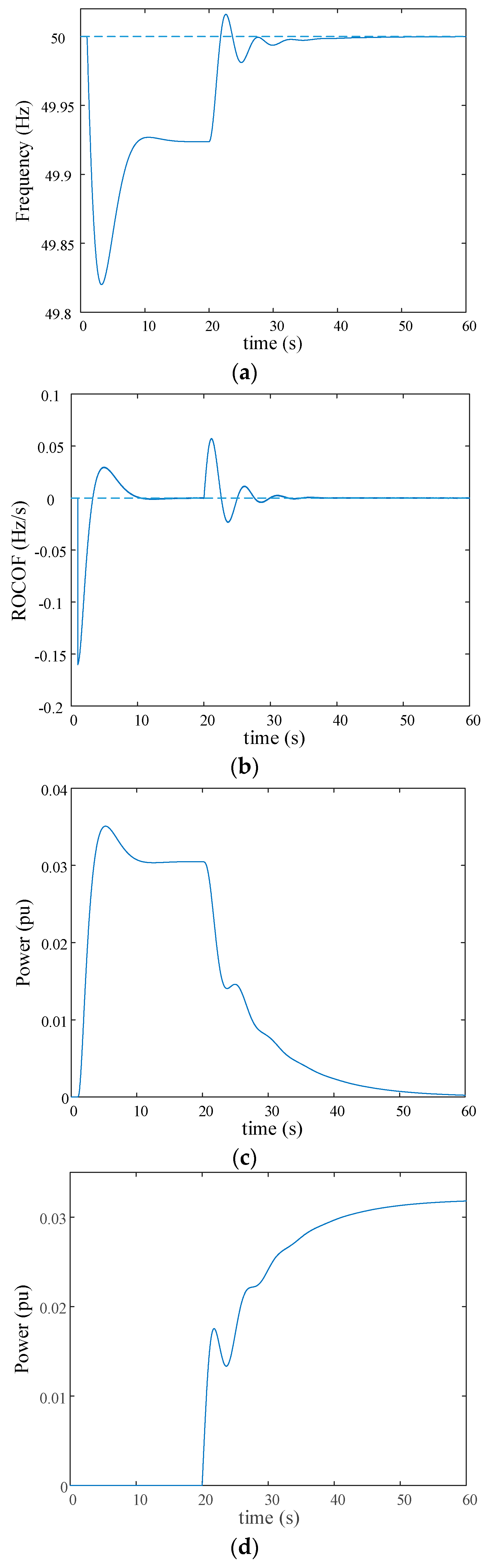
7. Conclusion

Based on the quantitative analysis of performance indices, this paper proposes a parameter tuning method for VSG-PEIs performing frequency control. From the above analysis, the following conclusions are made:

(1) From the perspective of the time scale and the activation, the frequency control is divided into two parts: the frequency response including IR and PFR, and the frequency regulation including SFR. Two dynamic systems are formed in different parts.

(2) By the effects of the dominant poles and zeros, the dynamic systems of the VSG-based PEIs in both parts are simplified into approximation models with second-order transfer functions. The performance indices are deduced from the reduced-order models.

(3) Different stages of frequency control kick in chronological order. In the proposed algorithm, the inertia constant is considered first for the ROCOF standard in the inertial response stage. Then the inertia constant and the speed droop are designed by checking the requirements of the nadir, the settling time, and settling frequency.

(4) In frequency regulation, the parameter of inertia and speed droop are inherited or readjusted from the previous part. The integral coefficient is determined according to the standard of SFR delivery time.

(5) The proposed algorithm can be utilized in two scenarios: (1) the parameter determination for the dominated PEIs in a stand-alone system, and (2) the equivalent parameter determination for a synchronous area with different units with inertia properties.

By the simulation results, the proposed method can fully satisfy typical performance standards.