Supervised Learning of Natural-Terrain Traversability with Synthetic 3D Laser Scans

Abstract

Autonomous navigation of ground vehicles on natural environments requires looking for traversable terrain continuously. This paper develops traversability classifiers for the three-dimensional (3D) point clouds acquired by the mobile robot Andabata on non-slippery solid ground. To this end, different supervised learning techniques from the Python library Scikit-learn are employed. Training and validation are performed with synthetic 3D laser scans that were labelled point by point automatically with the robotic simulator Gazebo. Good prediction results are obtained for most of the developed classifiers, which have also been tested successfully on real 3D laser scans acquired by Andabata in motion.

1. Introduction

Traversability is a key issue for motion planning of ground vehicles on unstructured terrain that has been addressed in different ways [1]. Among them, this relevant analysis can also be carried out with three-dimensional (3D) point clouds acquired at the ground level with stereo vision [2] or laser scanners [3].

3D laser scanners are of common use when moving on rough surfaces because they offer a great quantity of reliable information of the surroundings [4]. However, the resulting scans often have a complex structure and an uneven point density that decays with the distance to the sensor [5]. Nevertheless, these problems have not hindered autonomous navigation by processing raw point clouds directly [6,7].

Ground extraction is a process very related with traversability assessment, which is commonly performed just before scene segmentation [8]. Instead of designing specific segmentation procedures for floor detection [9], different machine learning techniques can be trained with spatial features computed right from the 3D point cloud [10,11].

Supervised learning usually employs hand-labelled points to obtain predictive models that can be applied to new data [12]. In this way, the Classification Learner App of Matlab has been employed to extract ground from 3D point clouds of an urban dataset [13]. Accordingly, a support vector machine was used to detect urban and rural roads with stereo vision [14].

However, tagging point by point real 3D data from ground vehicles on natural environments requires a laborious and error-prone effort [15]. In addition, to the best knowledge of the authors, there are no tagged repositories with this kind of data. As an alternative to manually-labelled data, learning from demonstration with 3D point clouds acquired from a teleoperated vehicle on traversable zones can be employed by a Positive Naive Bayes classifier [16], a Gaussian Process [17], or a support vector machine [18].

Moreover, synthetic depth data offers interesting opportunities for training traversability [19]. In this sense, virtual Lidar data generated with Matlab has been employed to build a neural network that classifies traversable terrain of planetary surfaces [20]. Similarly, in [21], a convolutional neural network has been trained to distinguish traversable patches from heightmap images obtained by the robotic simulator Gazebo [22].

To obtain natural-terrain traversability classifiers for 3D point clouds acquired by the mobile robot Andabata [23] on non-slippery solid ground, this paper develops the following main contributions.

• Synthetic 3D point clouds from Gazebo, that were previously labelled without errors [15], are employed for training and validation.
• The performance of seven potent supervised learning techniques from the free software Scikit-learn library [24] of the Python programming language is evaluated.
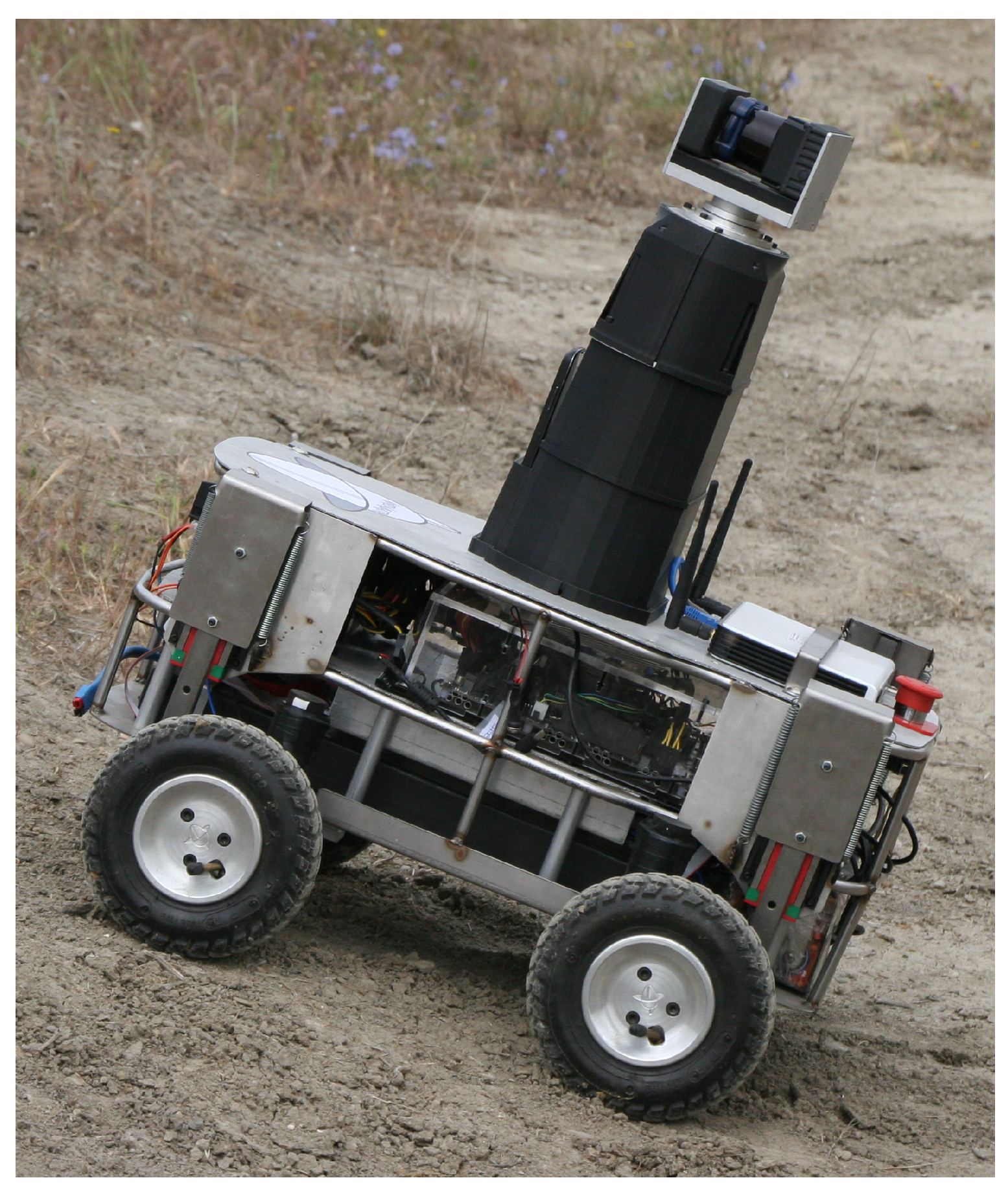
• The resulting classifiers are also tested with real data acquired, whereas Andabata was teleoperated on natural terrain.

The rest of the paper is organised as follows. The following section overviews the procedure used to obtain synthetic 3D laser scans with point traversability labels. Section 3 presents the training of various classifiers with these labelled point clouds. Then, Section 4 and Section 5 contain validation results for both simulated and real data, respectively. The paper ends with conclusions, acknowledgements and references.

2. Traversability-Labeling of 3D laser scans

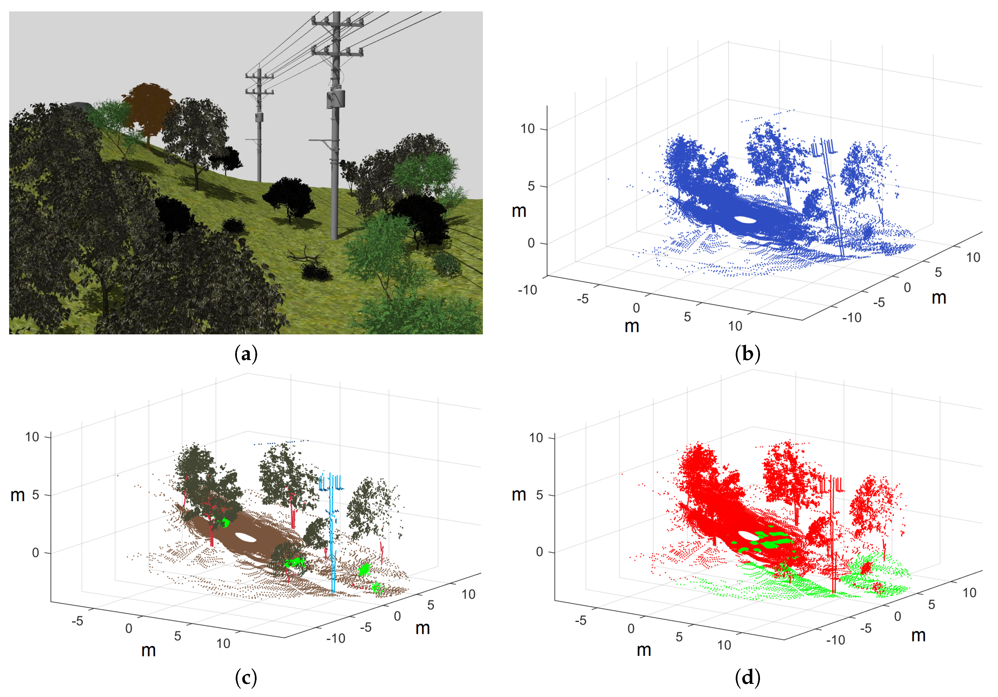
This section overviews how synthetic 3D laser scans of the mobile robot Andabata on natural environments can be labelled automatically [15]. Andabata is a ground vehicle for outdoor navigation, which is 0.67 m long, 0.54 m wide and 0.81 m high [23]. This skid-steered robot carries a 3D laser rangefinder on top and centered (see Figure 1), which is based on the unrestrained rotation of a commercial two-dimensional (2D) laser scanner around its optical centre [25].

The vertical and horizontal fields of view of the 3D sensor are 270° and 360°, respectively. The 3D sensor has inherited from the 2D scanner its vertical resolution of 0.25°, its $\pm 3$ cm accuracy and its range of measurements from 0.1 m to 15 m under direct sunlight [25]. The horizontal resolution of the 3D rangefinder depends on the turns performed by the entire 2D sensor and its turning speed. Once mounted on Andabata, the blind region of the 3D sensor is a cone that begins at its optical centre ( 0.723 m above the ground) and encompasses all the vehicle below [23].

The robotic simulator Gazebo [22] can be employed to obtain realistic point clouds of rough terrain from 3D rangefinders [3,19]. Figure 2 shows a general view of the natural environment generated with Gazebo, whose maximum dimensions are 150 m long, 150 m wide and 20 m high [15]. It contains natural elements like uneven ground, grass, bushes, rocks, trees and water. However, it also has artificial elements like tables, benches, fences, power lines and pavement. Five different zones can be distinguished inside: hills (A), a cave (B), a forest (C), a lake (D) and a park (E).

Apart from modelling the natural environment, Gazebo simulates the range and intensity measurements of the 2D laser scanner [22]. Successive rotations are applied to the 2D sensor around its optical center to obtain a full 3D scan [15]. The ranges are employed to calculate the 3D Cartesian coordinates of detected objects. Moreover, by taking into account the pitch and roll angles on the terrain [15], the whole point cloud is levelled to operate as Andabata does [23]. Besides, the intensity measurements are used to label each 3D point distinctively by assigning different reflectivity values to each natural or artificial element. In addition, points from the water element are removed from the 3D point cloud to emulate laser beam deflections [15].

Three laser scans with a horizontal resolution of 1° have been obtained for each zone of the natural environment by placing Andabata on different spots on the ground. Then, these synthetic scans are binarized in the following way; those points that belong to the ground, pavement and low grass (with a maximum height of 5 cm) are labelled as traversable and the rest as non-traversable. In addition, the inclination of every traversable point is estimated by computing the normal of the local plane fitted with the twenty nearest traversable neighbours. Finally, all the points with a slope greater than 20° (maximum inclination that Andabata can navigate) are re-labelled as non-traversable.

Figure 3 summaries the different stages required for labelling traversability:

(a)

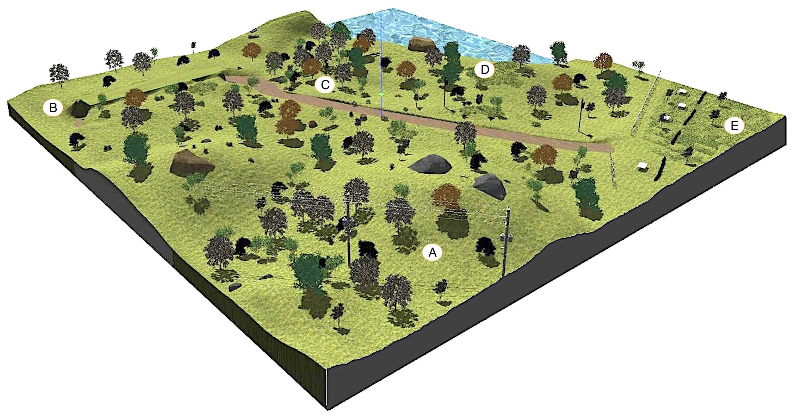
Represents a view of the hills zone (A) built with Gazebo [22].

(b)

Shows a simulated 3D scan acquired with Andabata. The empty circle on the ground at the center of the laser scan corresponds to the blind area of the 3D sensor.

(c)

Represents the previous scan once it has been levelled and its 3D points tagged with different colours according to their intensity values [15].

(d)

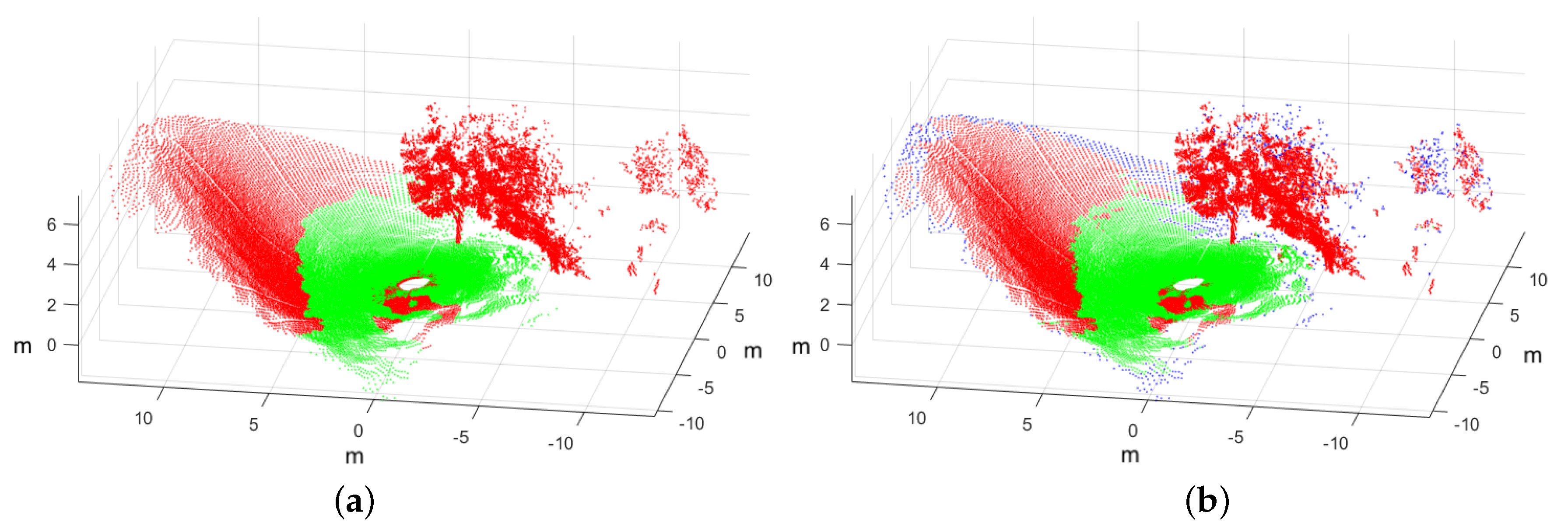
Shows the traversable points of the laser scan in green colour, and the rest in red. In this case, non-traversable points originate from trees, bushes, the electric line and very sloped terrain.

3. Training Terrain Traversability

The first step is to extract appropriate spatial features for traversability classification. Then, different supervised learning techniques can be trained.

3.1. Feature Computation

Spatial features are extracted for each 3D point from its neighbourhood, which is computed with a fixed proximity radius of 0.3 m. Those Cartesian points with less than five neighbours are discarded from feature calculation to ensure a minimum of information. Nearest neighbour search for every levelled point cloud is accelerated by using a 3D-tree data structure, which is built with the Python function KDTree from the Scikit-learn library [24].

The following combination of simple spatial features, which has been already used for reliable ground extraction [13], is employed for every 3D laser point.

• The minimum height coordinate among all the neighbours [11].
• The vertical orientation, which is obtained from an eigenvector of the lowest eigenvalue of the principal components analysis (PCA) [17].
• Scatterness, which is related with the value of the smallest eigenvalue from PCA [10].

PCA is sped up for each point neighbourhood with the Python compiler Numba (http://numba.pydata.org). Even so, the processing time of features still depends on the number of points of each 3D laser scan. To improve this time, by taking advantage of the four cores of the processor of Andabata (16 GB RAM, Intel Core i7 at 3.5 GHz), the Python library multithreading (https://docs.python.org/3/library/multiprocessing.html has been tested, but with disappointing results, and it has been discarded. Thus, for an average synthetic scan of 76,000 points, where ~3% of points do not have enough neighbours, data preprocessing is performed in 3.16 s.

3.2. Supervised Learning

Different classification algorithms from the Python library Scikit-learn [24] have been chosen to predict 3D point traversability using the above set of spatial features. This machine learning library was designed to operate with the numerical and scientific libraries of Python NumPy and SciPy, respectively [24].

Taking into account that it is not necessary to employ complex classification methods to extract ground accurately from 3D Lidar scans [13], seven relevant supervised learning techniques have been selected for training: Decision Trees (DT), Gaussian Naive Bayes (GNB), K-Nearest Neighbors (KNN), Linear Support Vector Machine (LSVM), Bagged Decision Trees (BDT), Random Forest (RF) and Gradient Boosted Trees (GBT). The last three are ensemble methods that combine various base estimators.

Ten of the fifteen generated 3D point clouds are dedicated exclusively to the training process. This error-free synthetic data contains a total of 743,346 points, where 721,616 comply with the minimum neighbourhood restriction. The training data is unbalanced because about 70% of points belong to the traversable class. This happens mainly because most of the laser points are acquired from the ground near Andabata.

Table 1. Training times for traversability classification.

Estimator	Acronym	Time (s)
Decision Trees	DT	3.3
Gaussian Naive Bayes	GNB	0.1
K-Nearest Neighbors	KNN	1.1
Linear Support Vector Machine	LSVM	136.3
Bagged Decision Trees	BDT	21.0
Random Forest	RF	8.1
Gradient Boosted Trees	GBT	41.3

shows the training times required by each estimator tuned with its default options. The most time-demanding methods are LSVM and GBT, whereas the less demanding methods are GNB and KNN. It is remarkable the big gap of 136 s between the best and the worst times. Nevertheless, these times are not critical for navigation because training is only performed once off-line.

4. Validating Traversability Classifiers

Five synthetic 3D point clouds, one per each zone of the natural environment, are employed for validation purposes exclusively. This data contains a total of 397,426 points where 385,959 have at least five neighbours. This validation data is also unbalanced with ~68% of points in the traversable class.

For all the classifiers, the prediction time for an average synthetic scan is almost negligible with respect to its preprocessing time with the exception of the KNN estimator that requires 0.2 s.

Table 2. Components of the confusion matrices for synthetic data.

Estimator	TP	TN	FP	FN
Decision Trees	111,912	252,446	10,007	11,594
Gaussian Naive Bayes	89,890	259,351	3102	33,616
K-Nearest Neighbors	111,538	256,915	5538	11,968
Linear Support Vector Machine	97,559	21,8384	44,069	25,947
Bagged Decision Trees	113,111	254,622	7831	10,395
Random Forest	112,547	257,396	5057	10,959
Gradient Boosted Trees	111,335	258,922	3531	12,171

contains the components of the confusion matrix of each trained classifier, where TP, FP, TN and FN stand for the number of true positives, false positives, true negatives and false negatives, respectively. True refers to points classified correctly and false to the opposite, whereas positive refers to the non-traversable class and negative to the traversable class.

To compare the performance of the binary classifiers, five accuracy indices for imbalanced data, computed by Scikit-learn functions (https://scikit-learn.org/stable/_downloads/scikit-learn-docs.pdf), are considered. The precision (PR), the recall (RE) and the F1 scores are the first, the second and the third indices, respectively:

$$PR=\frac{TP}{TP+FP},RE=\frac{TP}{TP+FN},F1=2\frac{PR·RE}{PR+RE}.$$

(1)

The fourth index is the balanced accuracy score (BA):

$$BA=\frac{1}{2}\left(RE+\frac{TN}{TN+FP}\right).$$

(2)

All the above indices vary between 0 and 1 for the worst and the best classification results, respectively. The last index is the Matthews correlation coefficient (MC):

$$MC=\frac{TP·TN-FP·FN}{\sqrt{(TP+FP)(TP+FN)(TN+FP)(TN+FN)}},$$

(3)

that ranges from −1 to 1, where −1 indicates an inverse classification, 0 a random prediction and 1 a perfect prediction.

Table 3. Balanced accuracy indices for synthetic data.

Estimator	PR	RE	F1	BA	MC
Decision Trees	0.918	0.906	0.912	0.934	0.871
Gaussian Naive Bayes	0.967	0.728	0.830	0.858	0.781
K-Nearest Neighbors	0.953	0.903	0.927	0.941	0.895
Linear Support Vector Machine	0.689	0.790	0.736	0.811	0.602
Bagged Decision Trees	0.935	0.916	0.925	0.943	0.891
Random Forest	0.957	0.911	0.934	0.946	0.904
Gradient Boosted Trees	0.969	0.901	0.934	0.944	0.906

includes the five accuracy indices for every estimator. In general, high accuracy is achieved, but the best performance comes from the RF and GBT classifiers and the least from the GNB and LSVM estimators.

Figure 4, Figure 5, Figure 6, Figure 7 and Figure 8 illustrate the results of applying the RF classifier to the five validation scans. Excellent estimations of both classes can be observed in red and green colours. Blue colour represents 3D points that have not been classified due to the lack of neighbours. These unclassified points are usually located far from Andabata, where scan density decreases.

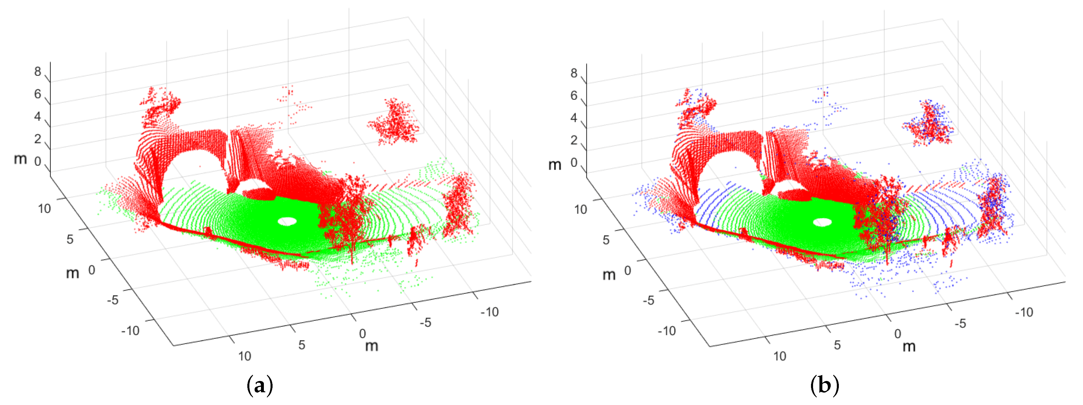
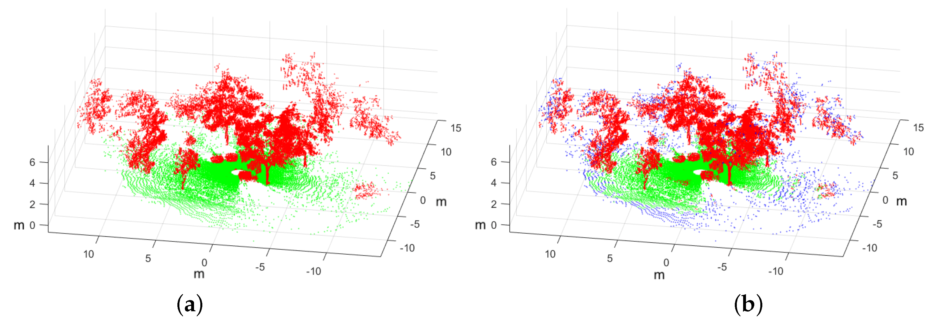
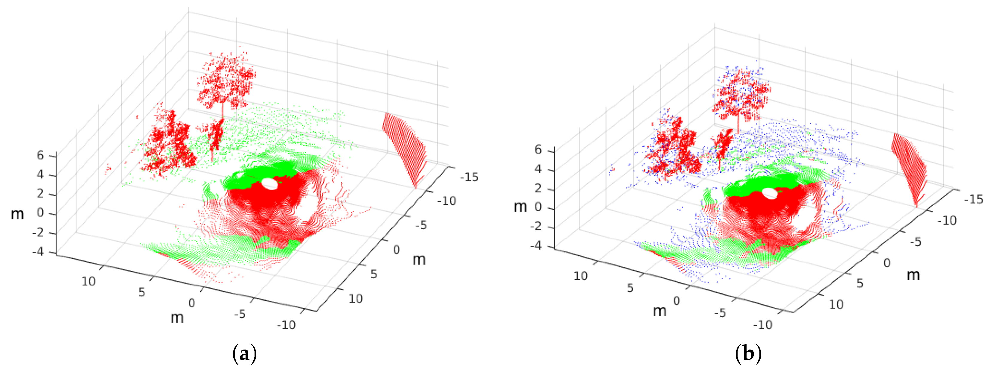
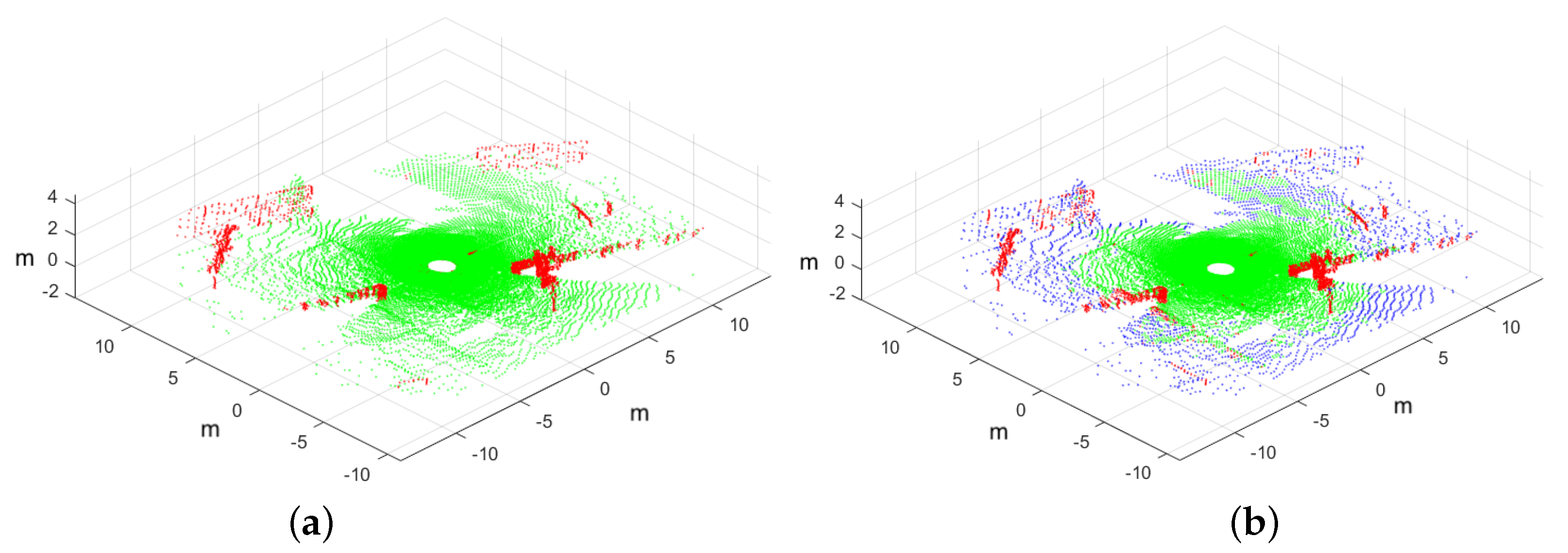
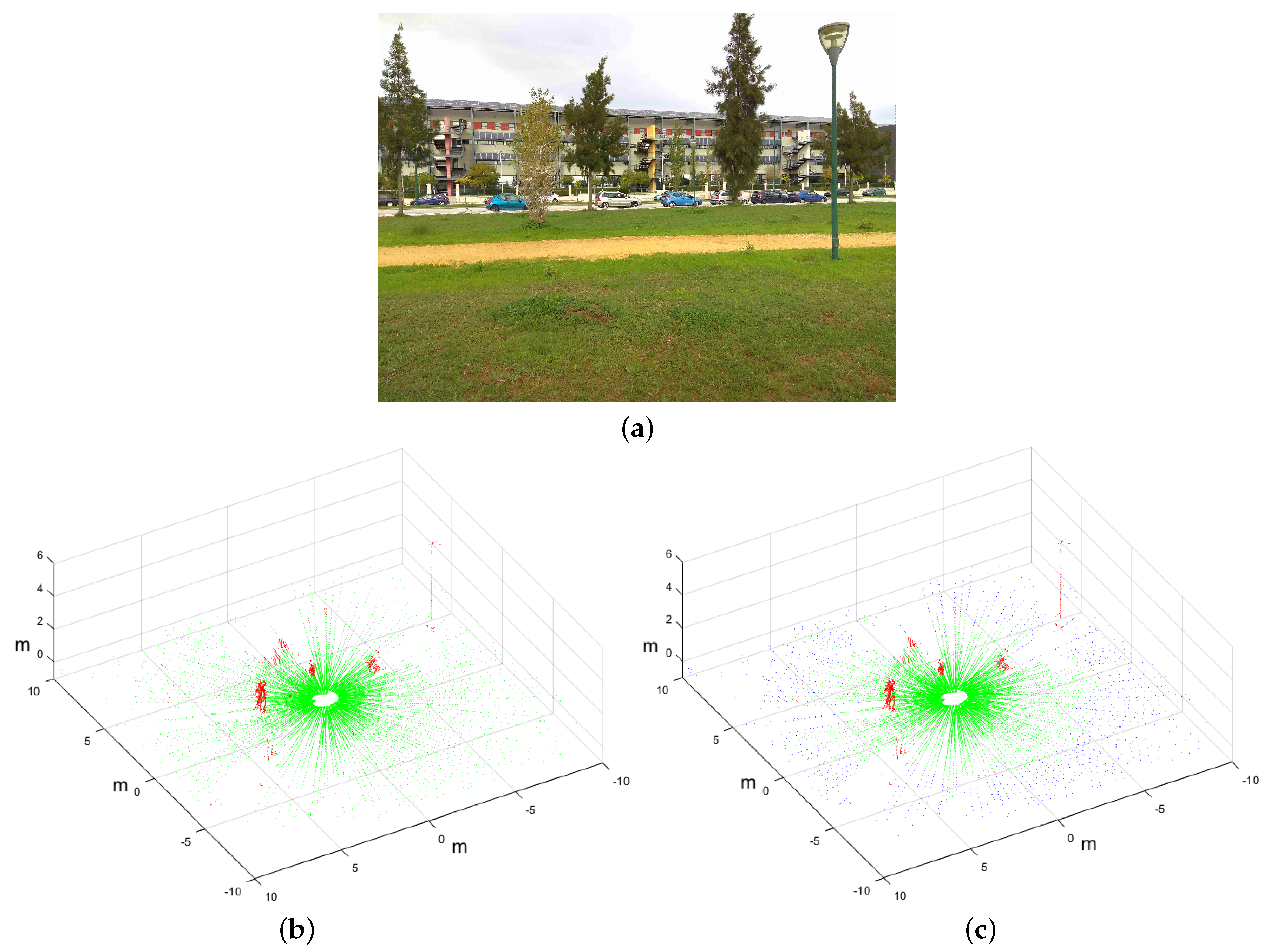
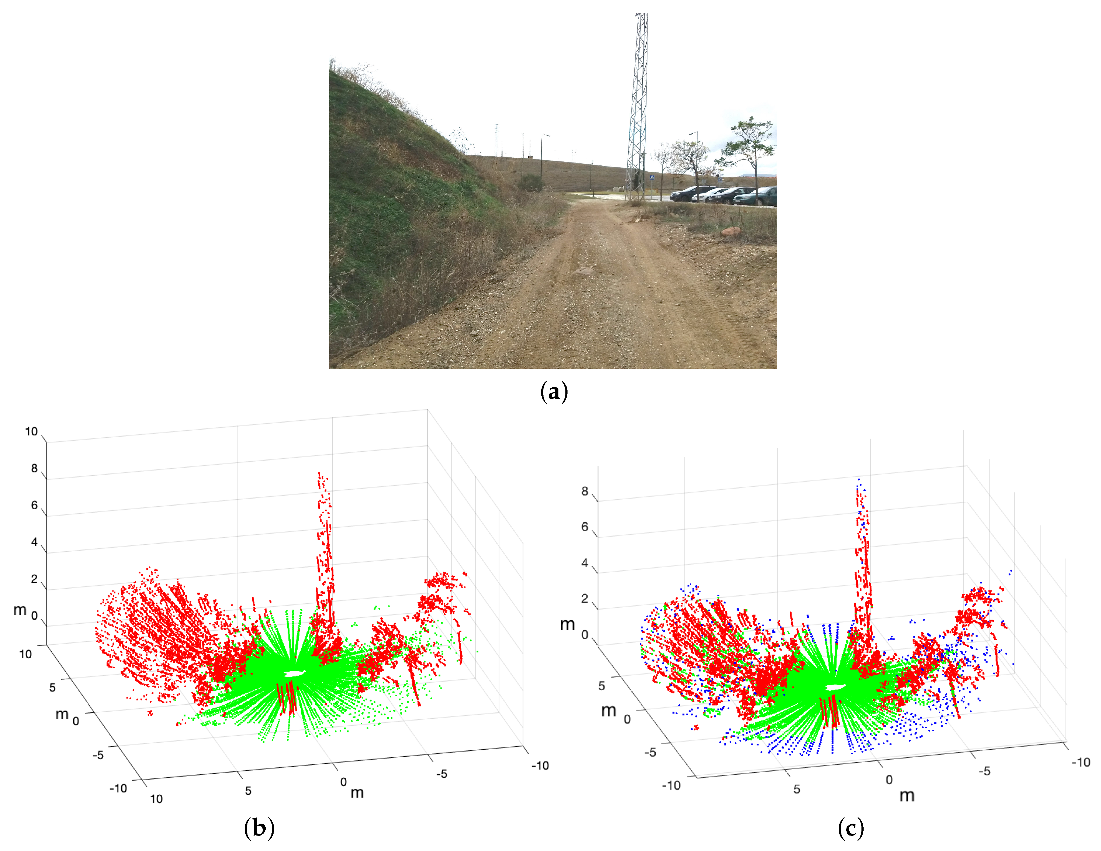
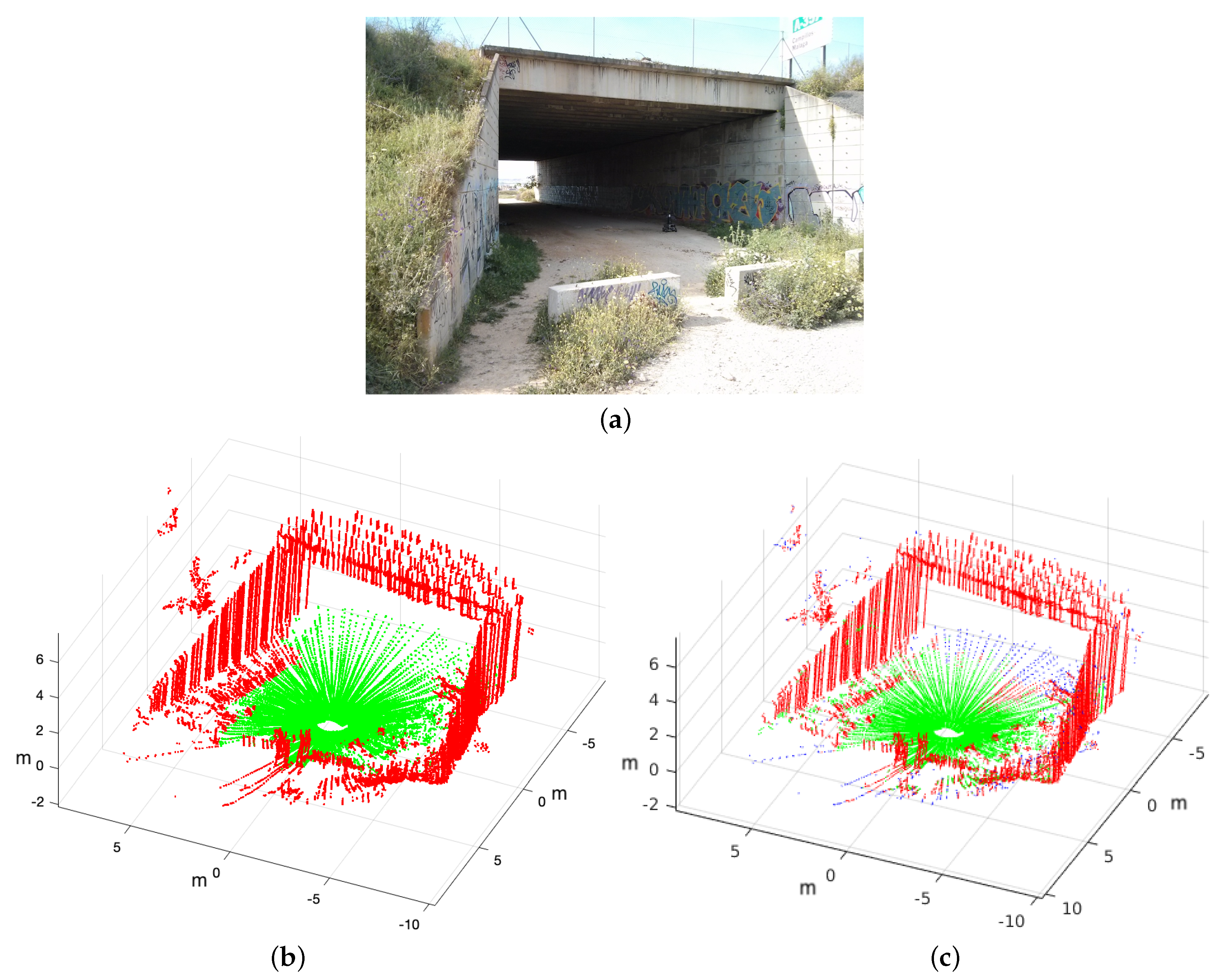
5. Classification Tests With Real 3D Laser Scans

Figure 9a and Figure 10a and Figure 11a show a park, a rural path and an underpass where Andabata has been teleoperated. For each scene, a levelled 3D point cloud with a horizontal resolution of 1.2° and without intensity data has been obtained in 3.75 s [23]. Sky visibility determines the number of points for each laser scan, ranging from 32,795 for the park to 83,183 for the underpass.

All this real data has been manually tagged to serve as ground truth (see Figure 9b and Figure 10b and Figure 11b). In these figures, it is noticeable that the blind area on the ground is reduced because Andabata was moving during scan acquisition. The hand-labelled data contains a total of 162,999 points, where 90,074 belong to the traversable class.

Feature extraction and traversability prediction for each scan can be obtained in 2.5 s for all the estimators with the exception of KNN that requires 2.7 s. In any case, these classification times make possible to process each 3D laser scan separately for autonomous navigation. Only 3215 points have not been classified due to the lack of five neighbours.

Table 4. Components of the confusion matrices for real data.

Classifier	TP	TN	FP	FN
Decision Trees	66,060	80,747	6918	6059
Gaussian Naive Bayes	51,110	83,541	4123	21,010
K-Nearest Neighbors	64,810	84,887	6679	3408
Linear Support Vector Machine	69,630	74,623	13,192	2339
Bagged Decision Trees	66,423	81,624	6027	5710
Random Forest	67,390	81,175	6475	4744
Gradient Boosted Trees	65,025	80,657	7893	6209

contains the confusion matrices obtained by each classifier. The balanced accuracy indices corresponding to this table can be found in

Table 5. Balanced accuracy indices for real data.

Classifier	PR	RE	F1	BA	MC
Decision Trees	0.905	0.916	0.911	0.919	0.836
Gaussian Naive Bayes	0.925	0.709	0.803	0.831	0.692
K-Nearest Neighbors	0.907	0.950	0.928	0.939	0.873
Linear Support Vector Machine	0.841	0.968	0.900	0.909	0.814
Bagged Decision Trees	0.917	0.921	0.920	0.926	0.852
Random Forest	0.912	0.934	0.923	0.930	0.859
Gradient Boosted Trees	0.892	0.913	0.902	0.912	0.822

. With real data, a slightly worst accuracy is achieved than with synthetic data, but it is still very high. The worst ranked estimators—GNB and LSVM—coincide with those pointed out in previous section. It also repeats as best ranked RF, this time accompanied by KNN.

Figure 9c and Figure 10c and Figure 11c illustrate the results of applying the RF classifier to the three real points clouds. Good classification results can be observed visually for all these scenes in these figures. Nevertheless, they contain errors such as some isolated green points on the slope near the rural path and on the vertical walls of the tunnel.

6. Conclusions

This paper has developed point-traversability classifiers for the 3D laser scans acquired by the mobile robot Andabata on natural environments. For this purpose, seven potent supervised learning methods from the Python library Scikit-learn have been employed. Apart from being very complete and using free software, this library has also facilitated the work flow to a great extent.

Furthermore, to perform training and validation, it has been necessary to use binary-tagged 3D point clouds obtained automatically with the robotic simulator Gazebo. This gravity-levelled data resembles closely that obtained by the 3D sensor of Andabata on non-slippery solid terrain. The main difference is that each synthetic point has associated a traversability label, that depends mainly on its intensity measurement.

For traversability assessment, three simple spatial features have been computed for every Cartesian point. However, feature extraction is a time-demanding process in Python that has been necessary to accelerate via compilation. On the contrary, prediction times, once obtained the features, are generally negligible. All in all, Andabata would be able to determine the traversability of a whole 3D laser scan well before the following 3D scan is available.

High accuracy indices for unbalanced validation data have been obtained for most estimators, outstanding the Random Forest method for both synthetic and real 3D point clouds. It has also been confirmed that the traversability classifiers, trained only with simulated data, can perform very well with real data.

Work in progress includes autonomous navigation of Andabata on natural environments based on the continuous traversability classification of successive 3D laser scans. It is also of interest to perform the tuning of hyper-parameters of classifiers to improve traversability estimations.

References

1. Papadakis, P. Terrain traversability analysis methods for unmanned ground vehicles: A survey. Eng. Appl. Artif. Intell. 2013, 26, 1373–1385. [Google Scholar] [CrossRef] [Green Version]
2. Kostavelis, I.; Nalpantidis, L.; Gasteratos, A. Supervised traversability learning for robot navigation. Lect. Notes Artif. Int. 2011, 6856, 289–298. [Google Scholar]
3. Zhang, K.; Yang, Y.; Fu, M.; Wang, M. Traversability assessment and trajectory planning of unmanned ground vehicles with suspension systems on rough terrain. Sensors 2019, 19, 4372. [Google Scholar] [CrossRef] [PubMed] [Green Version]
4. Zhu, Q.; Wu, J.; Hu, H.; Xiao, C.; Chen, W. LIDAR point cloud registration for sensing and reconstruction of unstructured terrain. Appl. Sci. 2018, 8, 2318. [Google Scholar] [CrossRef] [Green Version]
5. Bagnell, J.A.; Bradley, D.; Silver, D.; Sofman, B.; Stentz, A. Learning for autonomous navigation. IEEE Robot. Autom. Mag. 2010, 17, 74–84. [Google Scholar] [CrossRef]
6. Droeschel, D.; Schwarz, M.; Behnke, S. Continuous mapping and localization for autonomous navigation in rough terrain using a 3D laser scanner. Robot. Auton. Syst. 2017, 88, 104–115. [Google Scholar] [CrossRef]
7. Krusi, P.; Furgale, P.; Bosse, M.; Siegwart, R. Driving on point clouds: Motion planning, trajectory optimization, and terrain assessment in generic nonplanar environments. J. Field Robot. 2017, 34, 940–984. [Google Scholar] [CrossRef]
8. Douillard, B.; Underwood, J.; Kuntz, N.; Vlaskine, V.; Quadros, A.; Morton, P.; Frenkel, A. On the segmentation of 3D LIDAR point clouds. In Proceedings of the IEEE International Conference on Robotics and Automation (ICRA), Shanghai, China, 9–13 May 2011; pp. 2798–2805. [Google Scholar]
9. Vu, H.; Nguyen, H.T.; Chu, P.M.; Zhang, W.; Cho, S.; Park, Y.W.; Cho, K. Adaptive ground segmentation method for real-time mobile robot control. Int. J. Adv. Robot. Syst. 2017, 14. [Google Scholar] [CrossRef] [Green Version]
10. Lalonde, J.F.; Vandapel, N.; Huber, D.F.; Hebert, M. Natural terrain classification using three-dimensional ladar data for ground robot mobility. J. Field Robot. 2006, 23, 839–861. [Google Scholar] [CrossRef]
11. Kragh, M.; Jorgensen, R.; Pedersen, H. Object detection and terrain classification in agricultural fields using 3D Lidar data. Lect. Notes Comput. Sci. 2015, 9163, 188–197. [Google Scholar]
12. Xiong, X.; Munoz, D.; Bagnell, J.; Hebert, M. 3-D scene analysis via sequenced predictions over points and regions. In Proceedings of the IEEE International Conference on Robotics and Automation (ICRA), Shanghai, China, 9–13 May 2011; pp. 2609–2616. [Google Scholar]
13. Pomares, A.; Martínez, J.L.; Mandow, A.; Martínez, M.A.; Morán, M.; Morales, J. Ground extraction from 3D Lidar point clouds with the Classification Learner App. In Proceedings of the 26th Mediterranean Conference on Control and Automation (MED), Zadar, Croatia, 19–22 June 2018; pp. 400–405. [Google Scholar]
14. Bellone, M.; Reina, G.; Caltagirone, L.; Wahde, M. Learning traversability from point clouds in challenging scenarios. IEEE Trans. Intell. Transp. Syst. 2018, 19, 296–305. [Google Scholar] [CrossRef]
15. Sánchez, M.; Martínez, J.L.; Morales, J.; Robles, A.; Morán, M. Automatic generation of labelled 3D point clouds of natural environments with Gazebo. In Proceedings of the IEEE International Conference on Mechatronics (ICM), Ilmenau, Germany, 18–20 March 2019; pp. 161–166. [Google Scholar]
16. Suger, B.; Steder, B.; Burgard, W. Traversability analysis for mobile robots in outdoor environments: A semi-supervised learning approach based on 3D-Lidar data. In Proceedings of the IEEE International Conference on Robotics and Automation (ICRA), Seattle, WA, USA, 26–30 May 2015; pp. 3941–3946. [Google Scholar]
17. Santamaria-Navarro, A.; Teniente, E.; Morta, M.; Andrade-Cetto, J. Terrain classification in complex three-dimensional outdoor environments. J. Field Robot. 2015, 32, 42–60. [Google Scholar] [CrossRef] [Green Version]
18. Ahtiainen, J.; Stoyanov, T.; Saarinen, J. Normal Distributions Transform Traversability Maps: LIDAR-Only Approach for Traversability Mapping in Outdoor Environments. J. Field Robot. 2017, 34, 600–621. [Google Scholar] [CrossRef]
19. Shan, T.; Wang, J.; Englot, B.; Doherty, K. Bayesian generalized kernel inference for terrain traversability mapping. In Proceedings of the 2nd Conference on Robot Learning, Zurich, Switzerland, 29–31 October 2018; Volume 87, pp. 829–838. [Google Scholar]
20. Hewitt, R.A.; Ellery, A.; de Ruiter, A. Training a terrain traversability classifier for a planetary rover through simulation. Int. J. Adv. Robot. Syst. 2017, 14, 1–14. [Google Scholar] [CrossRef]
21. Chavez-Garcia, R.O.; Guzzi, J.; Gambardella, L.M.; Giusti, A. Learning ground traversability from simulations. IEEE Robot. Autom. Lett. 2018, 3, 1695–1702. [Google Scholar] [CrossRef] [Green Version]
22. Koenig, K.; Howard, A. Design and use paradigms for Gazebo, an open-source multi-robot simulator. In Proceedings of the IEEE-RSJ International Conference on Intelligent Robots and Systems (IROS), Sendai, Japan, 28 September–2 October 2004; pp. 2149–2154. [Google Scholar]
23. Martínez, J.L.; Morán, M.; Morales, J.; Reina, A.J.; Zafra, M. Field navigation using fuzzy elevation maps built with local 3D laser scans. Appl. Sci. 2018, 8, 397. [Google Scholar] [CrossRef] [Green Version]
24. Pedregosa, F.; Varoquaux, G.; Gramfort, A.; Michel, V.; Thirion, B.; Grisel, O.; Blondel, M.; Prettenhofer, P.; Weiss, R.; Dubourg, V.; et al. Scikit-learn: Machine learning in Python. J. Mach. Learn. Res. 2011, 12, 2825–2830. [Google Scholar]
25. Martínez, J.L.; Morales, J.; Reina, A.J.; Mandow, A.; Pequeño-Boter, A.; García-Cerezo, A. Construction and calibration of a low-cost 3D laser scanner with 360° field of view for mobile robots. In Proceedings of the IEEE International Conference on Industrial Technology (ICIT), Seville, Spain, 17–19 March 2015; pp. 149–154. [Google Scholar]
Figure 1. Andabata mobile robot equipped with its 3D laser scanner on the upper end.
Applsci 10 01140 g001
Figure 2. Overview of the natural environment built with Gazebo. Five different zones are marked with capital letters.
Applsci 10 01140 g002
Figure 3. A view of the hills generated with Gazebo (a), a synthetic 3D scan taken from this zone (b), its gravity-levelled and intensity-tagged point cloud (c) and the traversability-labelled 3D data (d).
Applsci 10 01140 g003
Figure 4. The validation scan on the hills (a) and the prediction results with RF (b).
Applsci 10 01140 g004
Figure 5. The validation scan at the entrance of the cave (a) and the prediction results with RF (b).
Applsci 10 01140 g005
Figure 6. The validation scan inside the forest (a) and the prediction results with RF (b).
Applsci 10 01140 g006
Figure 7. The validation scan near the shore of the lake (a) and the prediction results with RF (b).
Applsci 10 01140 g007
Figure 8. The validation scan on the park (a) and the prediction results with RF (b).
Applsci 10 01140 g008
Figure 9. A photograph of a park (a) and a real 3D point cloud from Andabata manually-tagged (b) and classified with RF (c).
Applsci 10 01140 g009
Figure 10. A photograph of a rural path (a) and a real 3D point cloud from Andabata manually-tagged (b) and classified with RF (c).
Applsci 10 01140 g010
Figure 11. A photograph of an underpass (a) and a real 3D point cloud from Andabata manually-tagged (b) and classified with RF (c).
Applsci 10 01140 g011