Efficient Management of Road Intersections for Automated Vehicles—The FRFP System Applied to the Various Types of Intersections and Roundabouts

Abstract

In the last decade, automatic driving systems for vehicles circulating on public roads have become increasingly closer to reality. There is always a strong interest in this topic among research centers and car manufacturers. One of the most critical aspects is the management of intersections, i.e., who will have to go first and in what ways? This is the question we want to answer through this research. Clearly, the goal is to manage the intersection safely, making it possible to reduce road congestion, travel time, emissions, and fuel consumption as much as possible. The research is conducted by comparing a new management system with the systems already known in the state of the art for different types of intersections. The new system proposed by us is called FRFP (first to reach the end of the intersection first to pass). In particular, vehicles will increase or decrease their speed in collaboration with each other by making the right decision. The vehicle that can potentially reach the intersection exit first.

1. Introduction

In the last few years, a number of companies (Google, Nissan, Tesla, etc.) and university research centers have been exploring the potential of automatic driving systems. In particular we are analyzing solutions for cooperation between vehicles, especially in the context of urban mobility. Undoubtedly, intersections represent one of the most complex and important scenarios to be managed for automatic vehicles. In fact, the level of interactions between vehicles, in these contexts, is very high. The vehicles will have to work together to optimize their crossing along the intersection, avoiding collisions and reducing the crossing times, emissions, and fuel consumption.

Poor management of the intersections certainly gives rise to possible road congestion, especially if there is a high presence of vehicles. The vehicles will therefore have to work together to modulate their speed in order to make the above mentioned possible.

The same scenario can be characterized by different conditions, for example, an intersection with a low presence of vehicles is certainly less critical in management than a strongly congested crossroads. In the latter case, the decisions made are of fundamental importance to avoid a critical increase in congestion.

This publication examines the development of a new intersection management system by comparing it with other state-of-the-art systems. Different types of intersections are analyzed, including roundabouts, in different vehicle flow conditions.

The approach used allows the management of collaboration between vehicles by means of vehicle-to-vehicle communication (V2V). This type of communication offers several advantages compared to other systems that can also be used in our system. For example, management based on the presence of the intersection manager (AIM) has the great disadvantage of requiring the installation of intersection managers at each intersection thus making the initial phase of real implementation of these systems at the urban level very complicated.

In a less critical and more extensive approach, the proposed system can provide a vehicle-to-cloud-edge communication (V2EC) for a coarser collaboration already at long distances. This can also be used for intelligent routing of vehicles based on the emission limits imposed according to the real traffic and weather conditions of the areas concerned. The use of this type of communication can also be used for optimization in the choice of routing according to different parameters such as, for example, the reduction of road congestion and the facilitation of pedestrian crossings. Furthermore, the possibility of collaborating over long distances allows us to limit abrupt variations in speed with a consequent reduction in consumption, CO₂ emissions and vehicle wear. Our work is focused on the management-collaboration of vehicles near the intersection (50–100 m) but it is also proposed to give an important starting point on the use of the same system in V2EC communication.

The publication is structured as follows. Section 2 describes the state of the art on the topics covered and then focuses on the motivations of the research carried out. In Section 3, our system is described in detail. Section 4 presents the results obtained. In Section 5, the conclusions are described. Section 5 exposes possible future works.

2. Related Work

The management of road intersections has become in recent years a fundamental theme in the management of automatic vehicles. Our research starts from an accurate analysis of the state of the art on this topic and then investigates possible solutions not yet explored and that can improve the efficiency of the intersection management algorithms.

Dresner and Stone in [1,2] present an intersection management reservation-based approach. The proposed system is based on the coordination of the intersection by the presence of AIM (Autonomous Intersection Management). The reservation policy is based on the FCFS system (first come, first served). This system results in some situations not very effective. The vehicle near the intersection could have a low speed compared to a more distant vehicle that, therefore, could potentially be the first to overcome the intersection with a minimum variation of the parameters of the vehicles involved. In this case the FCFS management could be more expensive in terms of time and efficiency (consumption, CO₂ emissions, vehicle wear).

Tsz-Chiu Au and Peter Stone present a system for managing vehicle parameters (acceleration, speed) at the intersections in FCFS systems managed by AIM [3].

The authors in [4] present a cooperative vehicle intersection control (CVIC) that manages the trajectories of the vehicles involved in an intersection so that the vehicles do not suffer collisions.

Azimi in [5] present a system based on vehicle-to-vehicle communications (V2V). The system provides for the crossing of vehicles at intersections in a synchronized manner. The presented protocol ballroom intersection protocol (BRIP) takes inspiration from the synchronization of the participants in the ballroom dancing. The system is very efficient as the vehicles will arrive at the intersection at the same time and will cross it at the same time occupying a very precise cell. The intersection is divided into cells never occupied by several vehicles at the same time. This system, although very efficient in homogeneous traffic conditions, has several limitations: all vehicles must have the same speed and same size; it is a system without priority and with difficult management of emergency; in non-homogeneous traffic conditions this system does not dispose of the traffic by balancing the congestions for their quick disposal. Furthermore, this approach cannot be used in certain types of intersections such as roundabouts, two lane intersections and connecting ramps.

In [6], a system based on the priority of lanes is proposed. The approach is based on three different states: full-priorized, semi-priorized, and fair-state. The system provides for the blocking of vehicles in non-priority lanes and does not manage any congestion conditions of the lanes.

In [7], the intersection management algorithm based on the FRFP approach is proposed (first to reach the end of the intersection first to pass).

The authors in [8] propose an approach based on an intersection manager that processes the parameters of all the vehicles periodically determining the optimal solution for crossing the intersection. The system is applied assuming straight trajectories of the vehicles that therefore will not turn at the intersections. An algorithm based on vehicle arrival priority is applied.

In [9] provides a general overview of the different projects used to adapt a factory vehicle, without access to low-level control systems, into a fully automated cooperative vehicle suitable to compete in GCDC2016. Communication and data degradation have been combined and validated experimentally in real-world scenarios, together with other vehicles with different implementations.

In [10] a system characterised by connected and autonomous vehicles (CAV) based on pre-assignment of slots is presented. A status adjustment area is created, at this area the vehicles are routed for a collision-free crossing.

A cooperative intersection control strategy is proposed in [11]. The proposed solution, called Cooperative Intersection Control (CIC), is based on the new concept of virtual platoon; platoons of vehicles that are in different lanes of the intersection and have different directional intentions. The performance of the presented strategy is evaluated and a comparison between the CIC and a controlled intersection with traffic lights is presented.

In [12] a platoon-based approach to the problem of cooperative management of intersections is proposed. It is stated that leveraging the platoon capabilities of autonomous vehicles could improve the efficiency of any policy at an intersection, in terms of average delay time per vehicle and reduce communication near intersections by a factor up to the average platoon size. A single 4-way intersection is examined in a simulated environment.

In [13] an intersection control algorithm is proposed assuming that there are bi-directional communication links with approaching vehicles. The intersection control node plans the crossing of the vehicles. The vehicle-intersection coordination problem is formulated as a mixed-integrated linear program (MILP).

In [14] a mechanism for estimating traffic by combining vehicle spacing information collected through the vehicle network and the calculation of the average spacing at a specific location over a short period of time is presented.

In [15] a possible solution to the problem of sudden road delays is discussed considering mobile traffic sensors installed directly on private and/or public transport and on volunteers’ vehicles. An IoT Cloud system for traffic monitoring and alarm notification based on OpenGTS and MongoDB is discussed.

In [16] it is proposed to analyse the performance of existing location-based routing protocols for the ad-hoc network of vehicles and to introduce the IDTAR (Intersection-based Distance and Traffic-Aware Routing) protocol.

In [17] the exploitation of vehicle storage capacity during a traffic jam is discussed and a scheme is proposed to create a Vehicle Data Centre (VDC) on a road segment (RS).

A number of conflicting assessment criteria are discussed in [18] and need to be balanced when designing an AIM system. Their priority-based design is introduced, where an intersection controller assigns priorities to incoming vehicles. Vehicles cross the intersection at the highest priority.

Our starting point is based on a V2V approach to overcome the large initial implementation limit that would require an intersection manager approach instead. Our research uses a FRFP protocol that allows a more natural management of trajectories over time. The system will be compared with different systems at the state of the art and in different conditions and in different types of intersections, including roundabouts. We will see how the proposed system minimizes the changes in the parameters of the vehicles involved so it is more effective in terms of consumption, emissions, wear, and time of crossing.

3. System Description

The idea developed is based on the principle that whoever has the potential to arrive first at the end of the intersection must be the one who has the priority to cross the intersection. This principle is believed to be very effective as the speed variations of the vehicles involved are certainly lower than other systems such as the FCFS system [1,2]. Just think of the case in which a vehicle, at a greater distance from the intersection than another, has a much higher speed than the one closest to the intersection. If the time required for the arrival at the end of the intersection of the fastest vehicle (t₁) is less than the time required by the other vehicle (t₂), priority will be given to the vehicle at a greater distance.

In the most optimistic case the fastest vehicle could pass the crossing even without requiring any reduction in the speed of the other vehicle involved in crossing the intersection; it would be very unnatural and certainly expensive to give priority to a very slow vehicle by imposing a strong reduction in the speed of the other vehicle. Therefore, it is believed that the system adopted can have significant advantages in terms of reducing the average crossing time, reducing fuel consumption, reducing vehicle wear and reducing CO₂ emissions.

We will then start to consider the simplest case of intersection, i.e. only two vehicles involved that can cross a single lane incident without being able to turn.

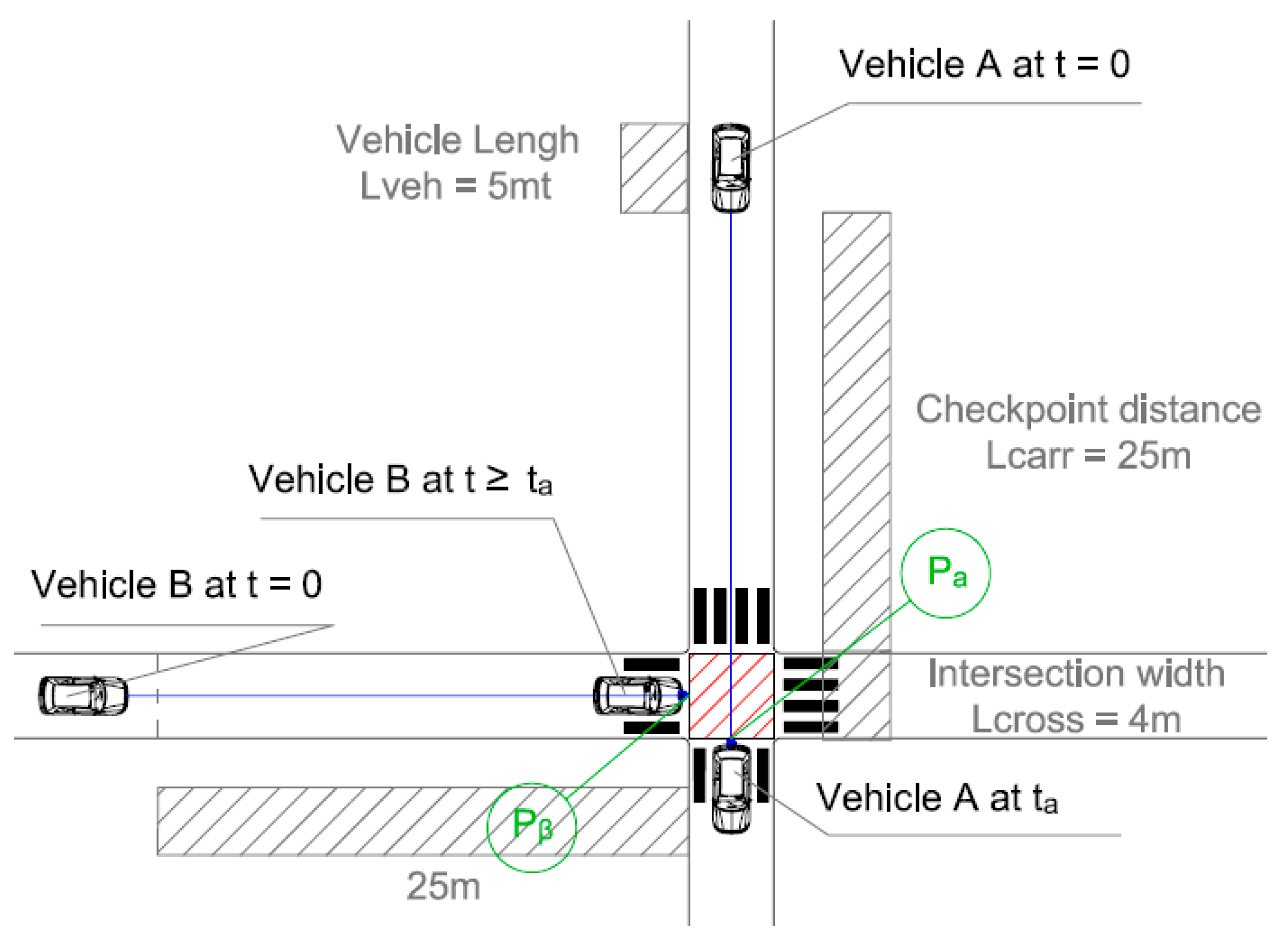
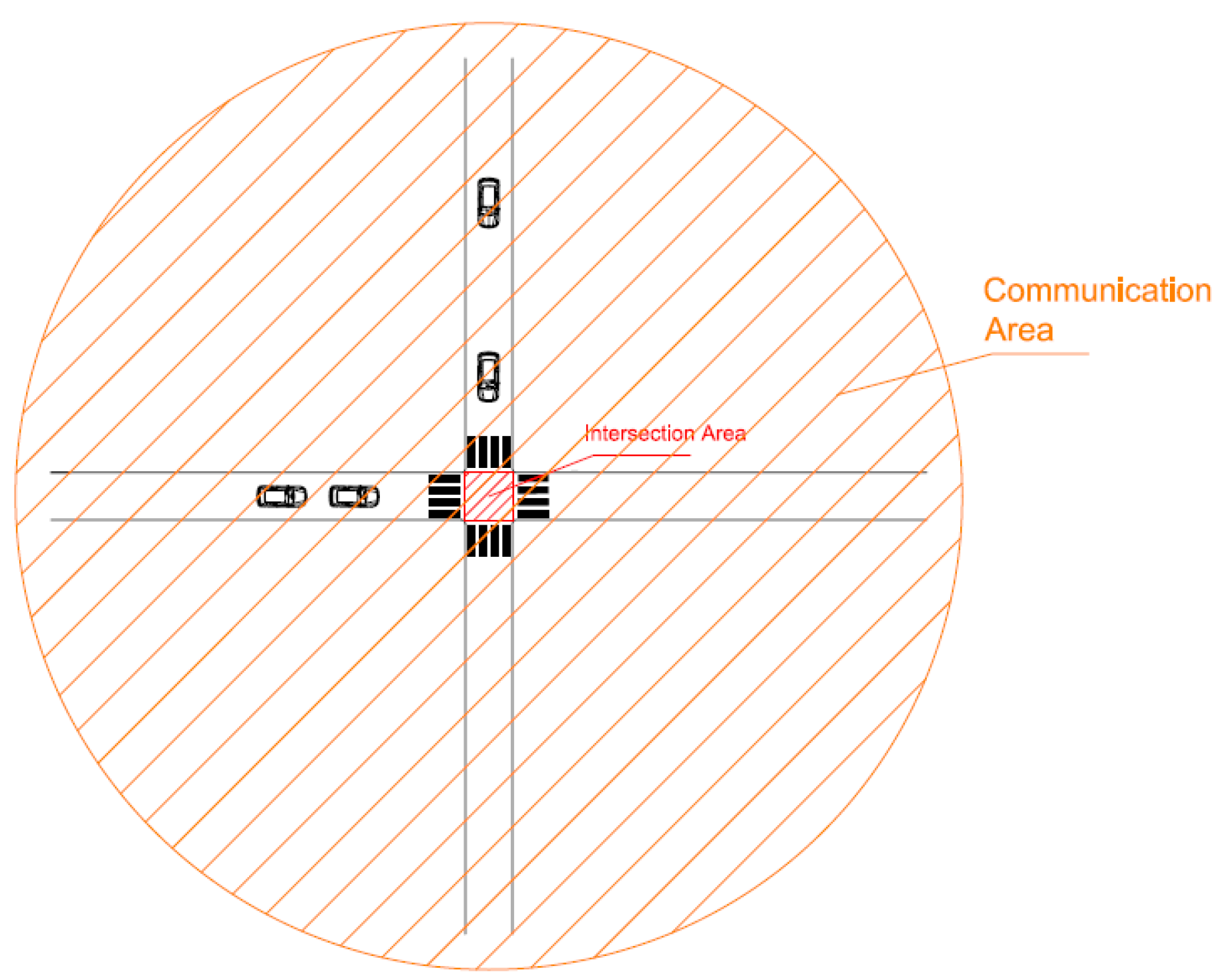
In Figure 1, the vehicle near the intersection communicate his position [S_A], its speed [v_A] and therefore the estimated arrival time at point P_A [t_A]. The vehicle that can arrive in less time has the priority. The vehicle with less priority will notice that it will pass through the intersection for second and calculate the deceleration [a_B] that it will have to maintain (a accelerated or decelerated motion is supposed to minimize fuel consumption and wear on the car). The vehicle with less priority must arrive at the beginning of the crossing at the same time or after the exit of the priority vehicle from the intersection (point P_A). In this case, as in the rest of our research, to ensure maximum security we are setting the entire intersection area as an area that will have to be occupied by only one vehicle at a time. The same system can be used by dividing the intersection area into cells. In this case we would increase the efficiency of the system but we would inevitably reduce the safety margins. In this case only the area occupied by the vehicles plus a small safety margin will have to be occupied only by one vehicle at a time.

Vehicle A communicates with its cadence [S_A, v_A, t_A] in the course of a path, so that vehicle B can constantly check that the calculation made at start does not have to be modified.

Vehicle A, assuming it moves at constant speed, will arrive at point P_A at the time ${\mathrm{t}}_{\mathrm{A}}=\frac{{\mathrm{S}}_{\mathrm{A}}}{{\mathrm{v}}_{\mathrm{A}}}$; where S_A is the distance between the vehicle and the P_A point (assuming the distance of the checkpoint from the intersection of 25 m [L_carr], the width of the intersection equal to 4 m [L_cross] and the length of the vehicle equal to 5 m L_veh)

$${\mathrm{t}}_{\mathrm{A}}=\frac{{\mathrm{S}}_{\mathrm{A}}}{{\mathrm{v}}_{\mathrm{A}}}=\frac{{\mathrm{L}}_{\mathrm{carr}}+{\mathrm{L}}_{\mathrm{cross}}+{\mathrm{L}}_{\mathrm{veh}}}{{\mathrm{v}}_{\mathrm{A}}}$$

(1)

where v_A is the speed of the vehicle A.

In the present case t_A = 8.5 s [we are assuming a constant speed of 4 m/s].

If Vehicle B can arrive to the end of the intersection in less time it will be the priority and will cross the intersection for first.

If the Vehicle B doesn’t have the priority it crosses the intersection for second.

Vehicle B will have to reach P_B point after a time greater than or equal to t_A. Applying the following formula the vehicle will be able to calculate the deceleration necessary to cross the intersection safely.

$$\mathrm{S}=\frac{1}{2}{\mathrm{a}\mathrm{t}}^2+{\mathrm{v}}_0\mathrm{t}+{\mathrm{S}}_0$$

(2)

Time t will be equal to t_A, space S will be equal to the distance between vehicle B and P_B point, speed V₀ will be equal to vehicle B speed (assumed constant), S₀ is the assumed starting point. So obtaining the following reverse formula for a it yields:

$$\mathrm{a}=2\times \frac{{\mathrm{S}}_{\mathrm{B}}-{\mathrm{v}}_{\mathrm{B}}{\mathrm{t}}_{\mathrm{A}}}{{\mathrm{t}}_{\mathrm{A}}{}^2}=2\times \frac{{\mathrm{S}}_{\mathrm{B}}-{\mathrm{v}}_{\mathrm{B}}\frac{{\mathrm{S}}_{\mathrm{A}}}{{\mathrm{v}}_{\mathrm{A}}}}{{\left(\frac{{\mathrm{S}}_{\mathrm{A}}}{{\mathrm{v}}_{\mathrm{A}}}\right)}^2}$$

(3)

The speed limit and the distance of the communication have to guarantee a feasible acceleration or deceleration. Assuming the constant speed V_B equal to 3.8 m/s Replacing the values in the example:

$$\mathrm{a}=2\times \frac{26.5-3.8\times 8.5}{{\left(8.5\right)}^2}=0.1605\mathrm{m}/{\mathrm{s}}^2$$

(4)

In this case, the vehicle B can accelerate to get to P_B point at the same time as the arrival of the vehicle A to the point P_A. If the value of a is positive the vehicle B can decide to accelerate to increase its speed and reduce the mean travel time. The decision may depend on the driving mode chosen and in any case known by the other vehicles as communicated together with the parameters. If the value of a is negative, vehicle B must apply the required deceleration. The accelerations or decelerations to be applied will be the less abrupt the greater the communication distance will be. Now suppose we have a more complex situation, i.e. an intersection always with 2 lanes but with many more vehicles involved. In this case, each vehicle, through V2V communication, will communicate its parameters to the other vehicles involved in the intersection.

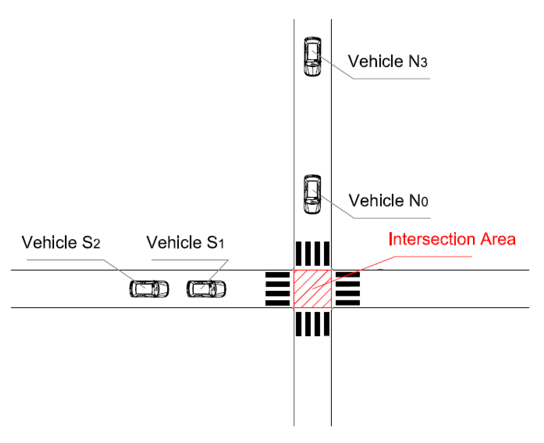
Then each of them will create a priority list based on the arrival time of each vehicle ${\mathrm{t}}_{\mathrm{x}}=\frac{{\mathrm{S}}_{\mathrm{x}}}{{\mathrm{v}}_{\mathrm{x}}}$ so, assuming the zero error communication system, each vehicle will know exactly the priority list. The list of priorities will be determined considering that if the system provides only one lane per direction, the vehicles of the same lane will necessarily have to respect the sequence of their positions.

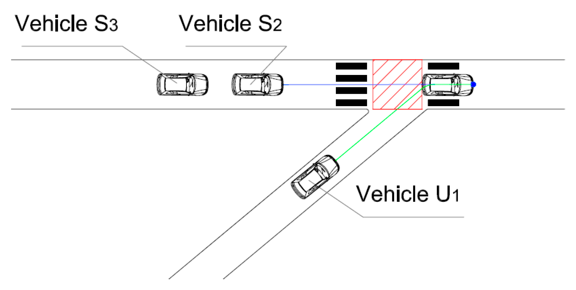
In Figure 2, for example, the priority will be the following [N₀, S₁, S₂, N₃, …] so the vehicle S₁ will adapt its speed according to the vehicle N₀, the vehicle S₂ will adapt its speed only to guarantee the minimum distance of safety from S₁, the vehicle N₃ will adjust its speed so as to arrive at the intersection at the moment when S₂ will arrive at the end of the intersection and so on.

Therefore, in the list of priorities the vehicles will distinguish the vehicle with conflict (coming from other lane) from those with no conflict (on the same lane).

The calculations described so far do not take into account two fundamental factors: maximum speed on the lane and maximum acceleration of each vehicle. In the implemented system the priority calculation is performed not considering the vehicle speed but its potential speed ($\mathrm{v}={\mathrm{v}}_0+\mathrm{a}\mathrm{\Delta }\mathrm{t}$). Clearly we must consider the speed limit and the performance in terms of maximum acceleration of the vehicle. In this case, in particular we might think that the vehicle can be set in different driving modes. A vehicle set in Eco drive will not want to apply high acceleration with the goal, for example, to reduce fuel consumption. In this case, the maximum acceleration desired by the vehicle will be taken into account in the calculations.

The time for calculating the priority and for calculating the acceleration/deceleration to be applied actually cannot be simply the one considered until now ${\mathrm{t}}_{\mathrm{x}}=\frac{{\mathrm{S}}_{\mathrm{x}}}{{\mathrm{v}}_{\mathrm{x}}}$. We must take into account various factors such as the maximum acceleration that the vehicle intends to apply and the maximum speed required for the lane in question.

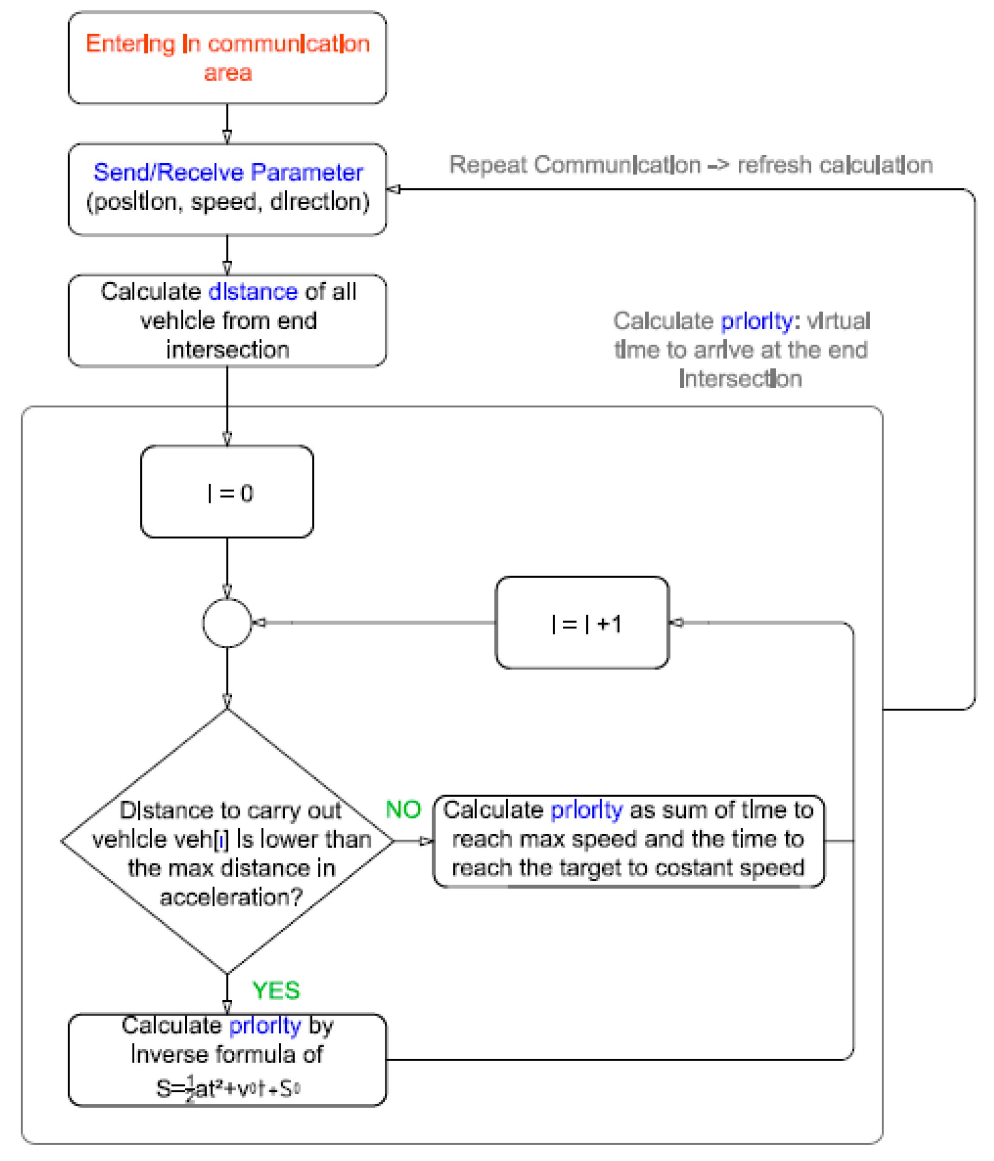
The procedure for calculating the priority for “regulation status”, as schematically shown in Figure 3, follows:

• Calculate the distance of vehicle list[i] from the end intersection [Dist]
• Survey the speed [Vel]

Determine priority as a time needed to carry out the vehicle from intersection.

Supply the maximum acceleration at the speed detected for a time t_max answer period of which the reached speed corresponds to the maximum speed or limit of the path.

If the distance to be left is lower than the maximum distance in acceleration, calculate the necessary time, which corresponds also to priority, between the inverse formula of

$$\mathrm{S}=\frac{1}{2}\mathrm{a}{\mathrm{t}}^2+{\mathrm{v}}_0\mathrm{t}+{\mathrm{S}}_0$$

(5)

where S is the distance to be made, a the maximum applicable acceleration, v₀ is the initial speed

$$\mathrm{t}=\frac{-{\mathrm{v}}_0+\sqrt{{{\mathrm{v}}_0}^2-2{\mathrm{a}}_{\max }\mathrm{S}}}{\mathrm{a}}$$

(6)

If the distance to be made is higher to the maximum distance in acceleration, calculate the necessary time, which corresponds also to priority, between the sum of t_max and t.

$$\mathrm{t}=\frac{\mathrm{Dist}-\mathrm{Dist}\_\max }{{\mathrm{v}}_{\max }}$$

(7)

where ${\mathrm{t}}_{\max }=\frac{{\mathrm{v}}_{\max }-{\mathrm{v}}_0}{{\mathrm{a}}_{\max }}$ from the inverse formula of ${\mathrm{v}}_{\max }={\mathrm{v}}_0+\mathrm{at}$.

Dist_max is the distance leaving after the time t_max.

When calculating the priority, it must also be taken into account that, regardless of speed, vehicles occupying the same lane must have sequential priority. The vehicle closest to the intersection will still have priority over the vehicles that occupy the same lane (except in the case where there are more lanes dedicated to overtaking). In this case, in calculating the priorities of the vehicle x we will not use the velocity v_x but we will use the speed of the vehicle that precedes it v_x–1.

At this point, we order the list of vehicles from two or more lanes according to the list of calculated priorities. We provide an example of priority list: [nord_1, right_1, right_2, nord_2, right_3, nord_3, ….]

Calculated vehicle priorities will apply the speed adjustment function by calculating the acceleration/deceleration to be applied for each of them. Then we apply function_decel between vehicles _[0] and _[1], after _[1] and _[2], and so on. If the vehicles are provided by the same lanes we do not modulate any of them. Other modules are as specified following: the vehicle_[0] will accelerate to the maximum value, the vehicle_[1] modules the speed that will be reached at the start of the crossing after the vehicle_[0] will be outside, and so on for the other vehicles _[i] and _[i+1].

In this function, the time needed to the priority vehicle to exit from intersection is calculated:

$$\mathrm{t}=\mathrm{Dist}/\mathrm{speed}$$

(8)

For safety we consider that the vehicle is moving at the speed communicated without applying any acceleration. Then, we calculate the acceleration with the following form:

$$\mathrm{a}=2\times \frac{\mathrm{S}-{\mathrm{v}}_0\mathrm{t}}{{\mathrm{t}}^2}$$

(9)

where S is the distance from the start of the intersection an v₀ is the speed of the non-priority vehicle, when the time t is calculated by the previous form (time so that priority vehicle can reach the end of crossing).

The system described up to this point, although it is very efficient, presents a critical point. Let’s assume we have a lot of high speed Sx vehicles and only one very low speed vehicle at the intersection. In this limit condition we may find ourselves never to witness the crossing of the Nx vehicle.

To deal with these situations in conjunction with, in general, situations of particular intersection congestion, we have introduced three different work states. The one seen so far represents the “regulation state” and manages the intersection as long as there are no blocking or intersection congestion situations. In case of congestion and/or self-intersection blocking we will talk about “balance state”. In case of post-intersection congestion, for example due to a vehicle failure, we will talk about “Freeze state”.

The “balance state” status is introduced both to eliminate the previously presented case and to more effectively manage high congestion characterized by many low-speed vehicles. The last state “freeze state” provides that since there is a post-intersection block all vehicles in that direction will remain in the pre-intersection lane giving priority to vehicles with free lanes.

The state “balance state” was initially implemented with a platoon algorithm, thus foreseeing the passage of vehicles no longer according to the list of priorities according to the “regulation state” but balancing the crossing of a number of vehicles per lane depending on the percentage of vehicle presence on lane interested. For example, if we have 10 vehicles involved in a lane and five vehicles in the other, then double the number of vehicles in the lane that is more congested, then the other group will pass. For example, two vehicles N and four S vehicles. From the simulations carried out, this type of approach was less efficient than the FCFS system, which was then adopted for the Balance status.

Conditions that imply the state of balance clearly in an evolution of the system may differ depending on the type of intersection. In our implementations we have imposed a percentage threshold of the presence of vehicles on one lane compared to the others involved.

Balance State: when we have a congestion or when the gap between the vehicles blocks the passage from the other lane.

If the vehicle_[1] is stopped and it must restart to reach the end of the crossing we then assume that the initial speed [v_i] is 0 and a maximum acceleration a.

The time necessary to cross (t_c) is:

$${\mathrm{t}}_{\mathrm{c}}=\sqrt{\frac{2\mathrm{S}}{\mathrm{a}}}$$

(10)

where: $\mathrm{S}=\frac{1}{2}{\mathrm{at}}^2+{\mathrm{v}}_{\mathrm{i}}\mathrm{t}$

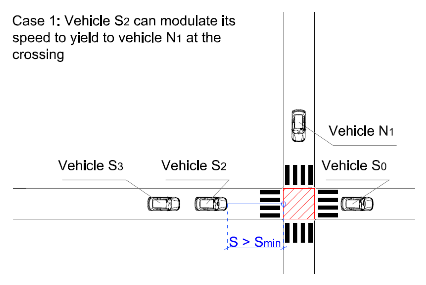
We can consider two different scenarios:

• [Figure 4, Regulation State] The vehicle_[2] has a long gap with the vehicle_[0] and has the time t_i to permit the crossing of the vehicle_[1]; in this case t_i, the time required by vehicle S₂ to arrive at the beginning of the intersection must be greater than or equal to t_c, the time required by vehicle N₁ to reach the end of the intersection.
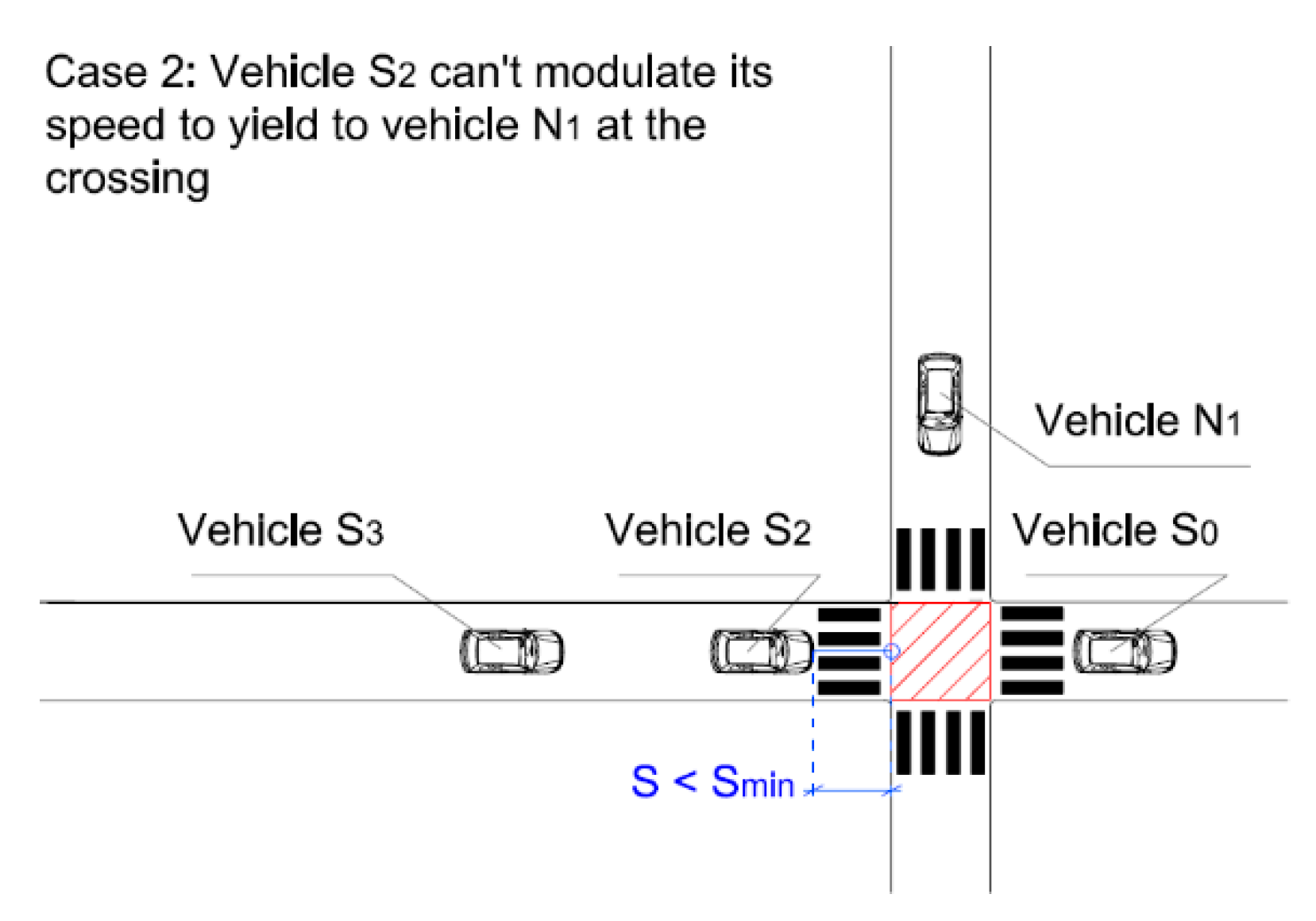
• [Figure 5] The vehicle_[2] has a short gap with the vehicle_[0] and the priority may never be released to the vehicle_[1]. The necessary minimum time to crossing the intersection of vehicle_[1] is given by following inverse formula:

  $${\mathrm{S}}_1=\frac{1}{2}{\mathrm{at}}_{\mathrm{cmin}}{}^2+{\mathrm{v}}_{\mathrm{i}}{\mathrm{t}}_{\mathrm{cmin}}$$

  (11)

where a is the maximum acceleration applicable, S₁ is the distance of vehicle_[1] from the end of the intersection, t_cmin is the minimum time required from vehicle_[1] to reach the end intersection.

The real solution of the follow formula is the minimum time required to guarantee the crossing the intersection of vehicle_[1]

$${\mathrm{t}}_{\mathrm{cmin}}=\frac{-{\mathrm{v}}_{\mathrm{i}}\pm \sqrt{{\mathrm{v}}_{\mathrm{i}}{}^2+2{\mathrm{aS}}_1}}{\mathrm{a}}$$

(12)

The maximum time required to vehicle_[2] to arrive at begin of the intersection is given by the following inverse formula:

$${\mathrm{S}}_2=\frac{1}{2}{\mathrm{at}}_{\max }{}^2+{\mathrm{v}}_{\mathrm{i}}{\mathrm{t}}_{\max }$$

(13)

where a is the maximum deceleration applicable, S₂ is the distance of vehicle_[1] from the begin of the intersection, t_max is the maximun time required from vehicle_[2] to reach the begin intersection.

The real solution of the follow formula is the maximum time required to reach the begin intersection of vehicle_[2]

$$t_{max}= \frac{-v_i\pm \sqrt{v_i{}^2+2a{S}_2}}{a}$$

(14)

If t_max will be greater than t_cmin the vehicle_[1] will be able to have priority and therefore will be able to cross the intersection; otherwise the vehicle_[1] may never have priority.

To guaranteed the release of the priority, the minimum distance of vehicles from the begin intersection must be over:

$$S_{min}= \frac{1}{2}a{t}_c{}^2+v_i{t}_c$$

(15)

where t_c is the time request to vehicle_[1] to reach the end of intersection.

To manage case 2 we’ll change the status from regulation in balance.

The basic concepts remain almost identical but with the appropriate considerations in intersections of different types. The system has also been applied to on-ramp systems, 8 lanes intersections and roundabouts.

Figure 6 shows the case of the on-ramp intersection. In this case, the different vehicle trajectories must be considered to arrive at the end of the intersection. In general, vehicles coming from the low lane must travel a greater distance to reach the end of the crossing. Therefore, in the formulas previously presented, the relative distances between the vehicles and the end intersection must be entered considering the trajectories that the vehicles will carry out.

In the systems applied to eight-lane intersections, the algorithm has been applied considering also the possibility of vehicles to turn at the intersection. In this case, obviously, the different distance of travel must be considered to exit the intersection zone with respect to a vehicle that continues straight.

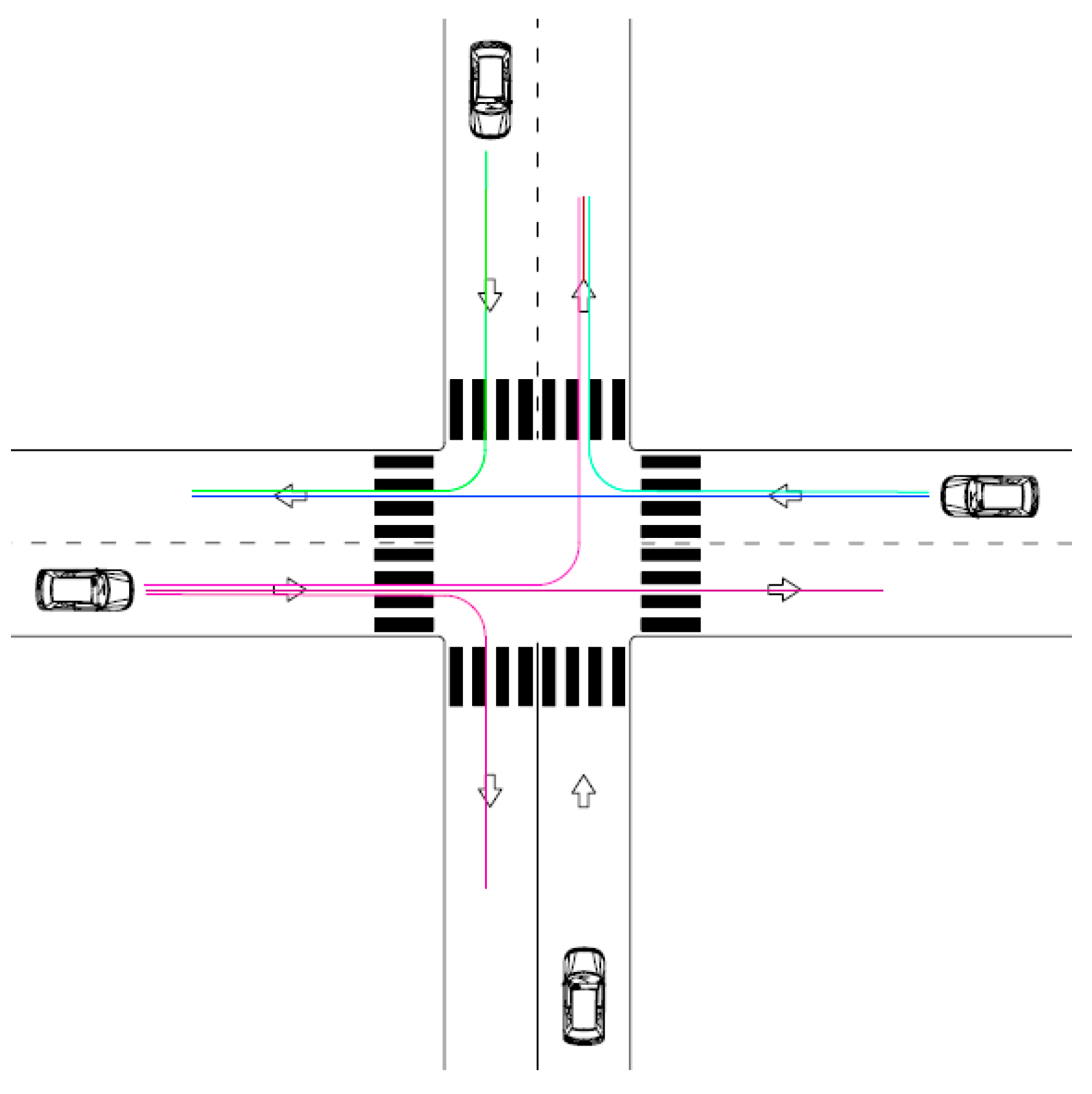
Moreover, in more complex systems like eight-lanes intersections (Figure 7), all possible trajectories must be considered.

In this type of crossing, each vehicle can travel three different trajectories, in total so there will be 12 different possible trajectories. For each possible trajectory it is necessary to identify the trajectories without any collisions between them and therefore the critical ones with possible collisions that must be managed by the vehicle speed control. The system determines the list of priorities by calculating the estimate of the time needed to reach the end of intersection point. At this point the vehicle that holds the priority passes first and in cascade all adapt to the vehicle that precedes them. In the modulation of speed, the vehicles, to adapt to the competitors that precede them, will take into account the fact that the trajectories of the other vehicles may or may not be compatible with their route.

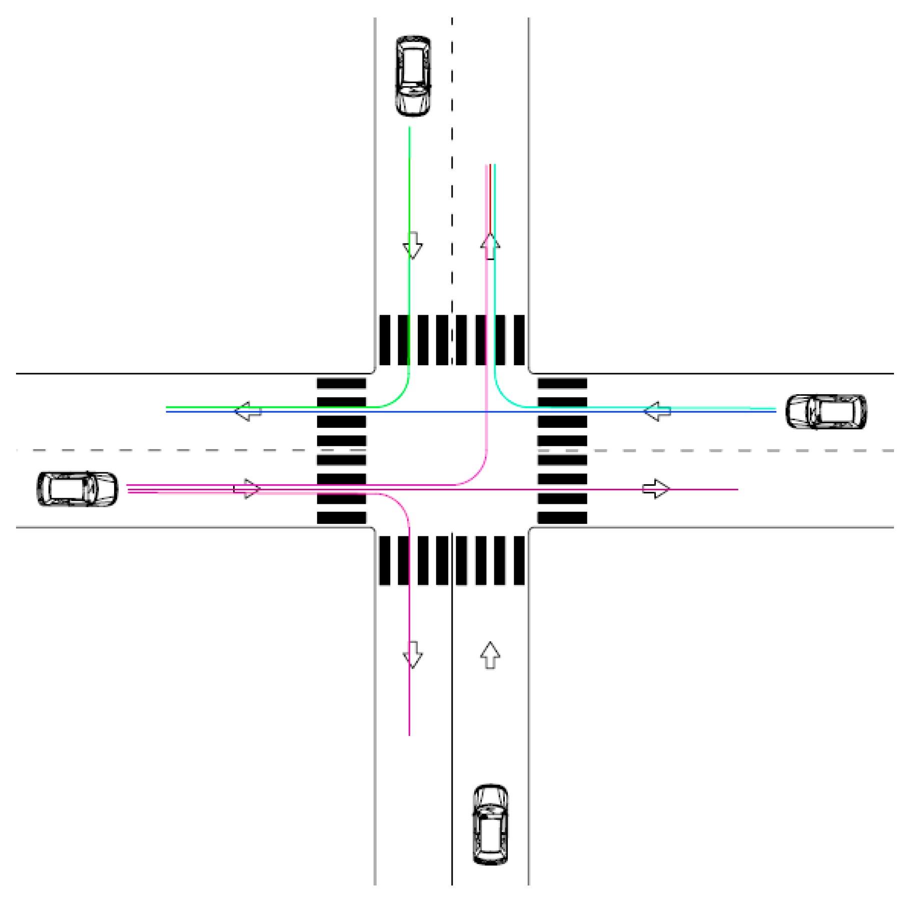
Figure 8 shows the collision-free trajectories with vehicles in the right direction, direction highlighted in violet. In this case the collision-free paths are those of the vehicles in the down_left, left, left_up, right_down and right up direction.

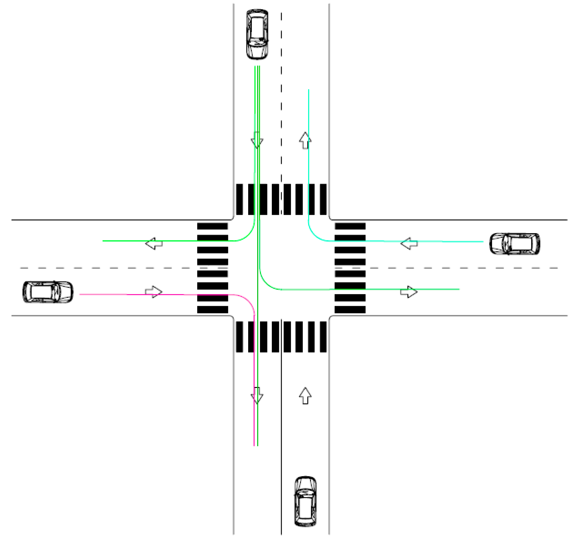
Figure 9 shows the trajectories without collisions with the vehicles in the down-right direction, the direction highlighted in green. In this case, the collision-free paths are those of the vehicles in the down_left, down, left_up, and right_down directions.

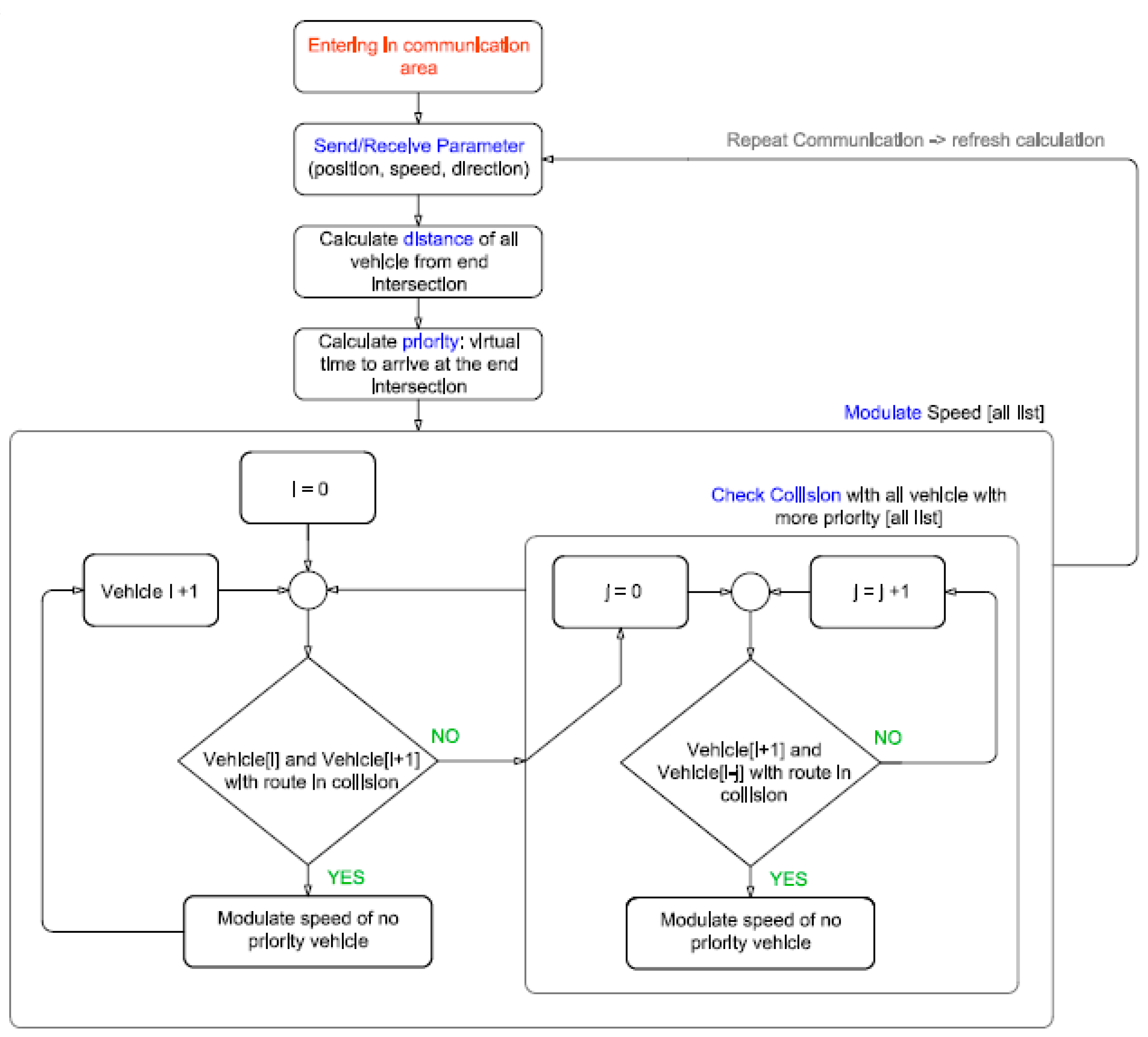
Therefore, all possible collisions in the possible routes must be detected, in this case 12, and then manage the regulation state according to the fact that the two consecutive priority vehicles can have collisions or not. In the event of a possible collision we will adjust the speed of consecutive vehicles. Otherwise the vehicles will safely cross the intersection without any adjustment. Figure 10 follows the block diagram of the implemented system.

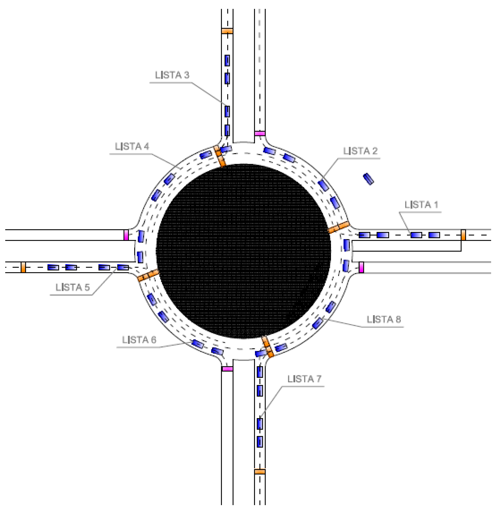
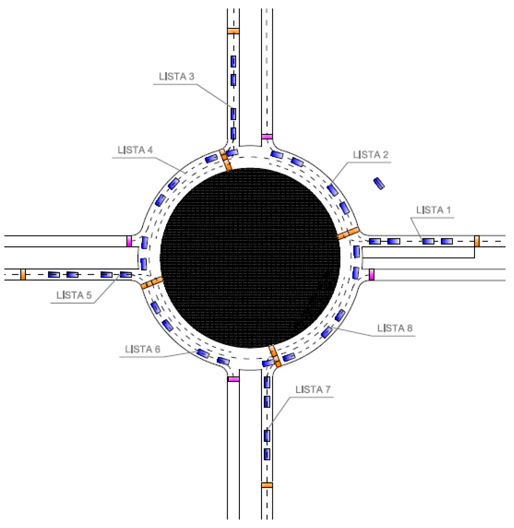
The same system can be applied at roundabouts. In this case, the system is complicated because basically we have a system composed of crossings. In the example in Figure 11, the roundabout has 4 intersections.

The principle remains the same, but in this case we have to manage 4 different intersections. Referring to the figure, the vehicles of list 1 and list 8 will have to work together to form list 2. It will take into account both the presence of vehicles that will exit the roundabout before meeting the vehicles on list 1 and the lanes to be occupied according to path that you will have to follow. The vehicles ready to exit the roundabout will occupy the most external lane, the others the internal one. In the same way the vehicles of the list 2 will collaborate with those of the list 3 and so on. The optimization of the roundabout certainly has as main objective to dispose as quickly as possible the cars already inside the same. In fact, faster entry into disposal will lead to an inevitable saturation with a consequent slowing down of the vehicles involved. As we will see later, from the simulations performed, the use of roundabouts is not suitable for optimizing travel time in the presence of driverless vehicles.

4. Results

The developed algorithm has been simulated and compared to different state-of-the-art systems. In particular, it has been compared with the classic traffic light system, with the FCFS system, with the Ballroom system and with the priority system on the lane. Four different intersection systems have been implemented: two-lane intersection, on-ramp, eight-lane intersection, and roundabout. The implemented systems have been tested under various congestion conditions. In our simulations, we have used SUMO (Simulation of Urban MObility) and netedit to implement the intersection system. All the simulations were performed by setting a maximum speed of 13 m/s, a minimum gap between vehicles equal to 1 m, a maximum acceleration of 4 m/s² and a maximum deceleration of 3 m/s². The communication system between vehicles is considered to be devoid of any error and a distance of 40 meters from the intersection is considered. The refresh time of the communication is equal to 1 s.

Intersection type 1 (two lanes) (Figure 12):

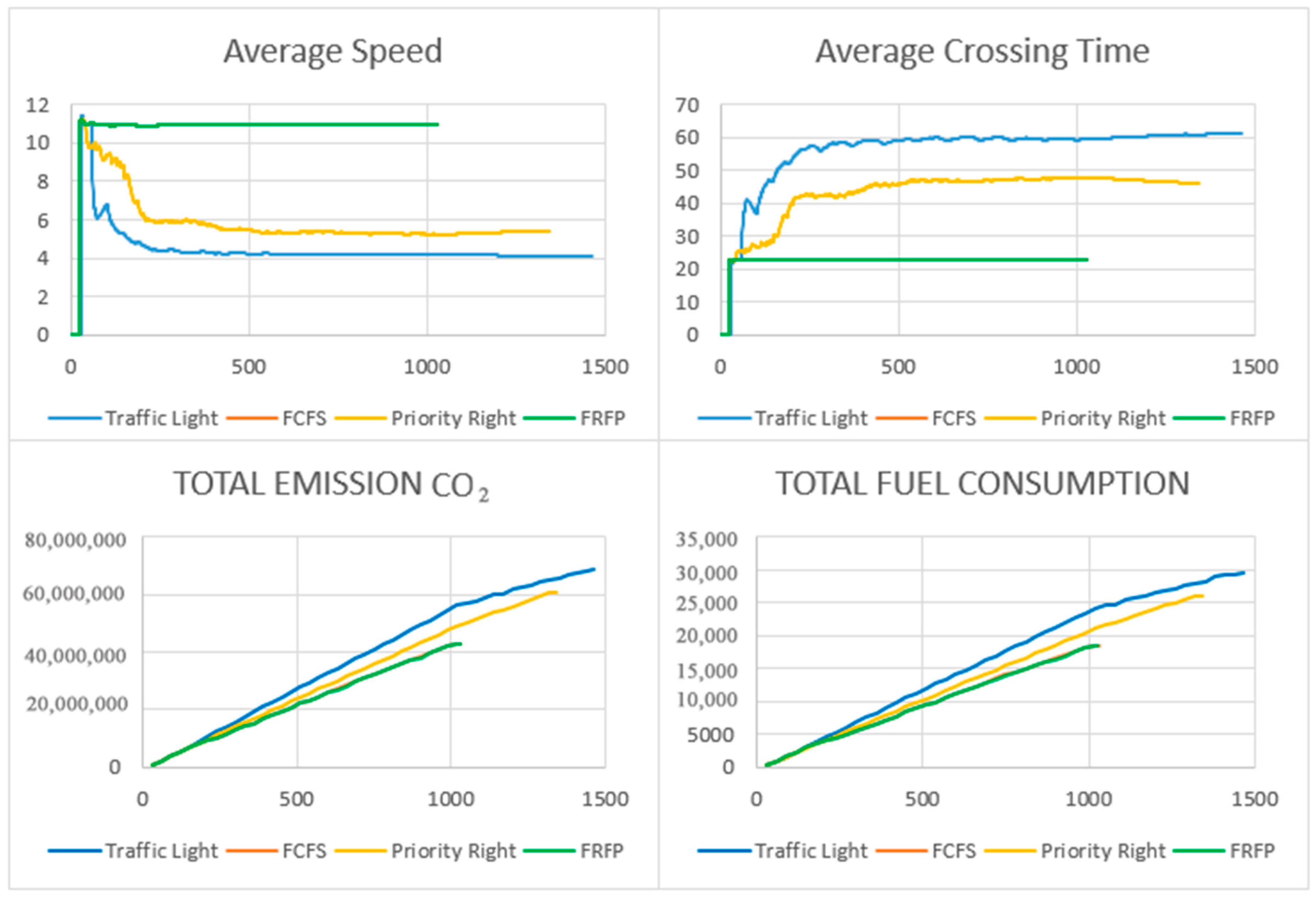
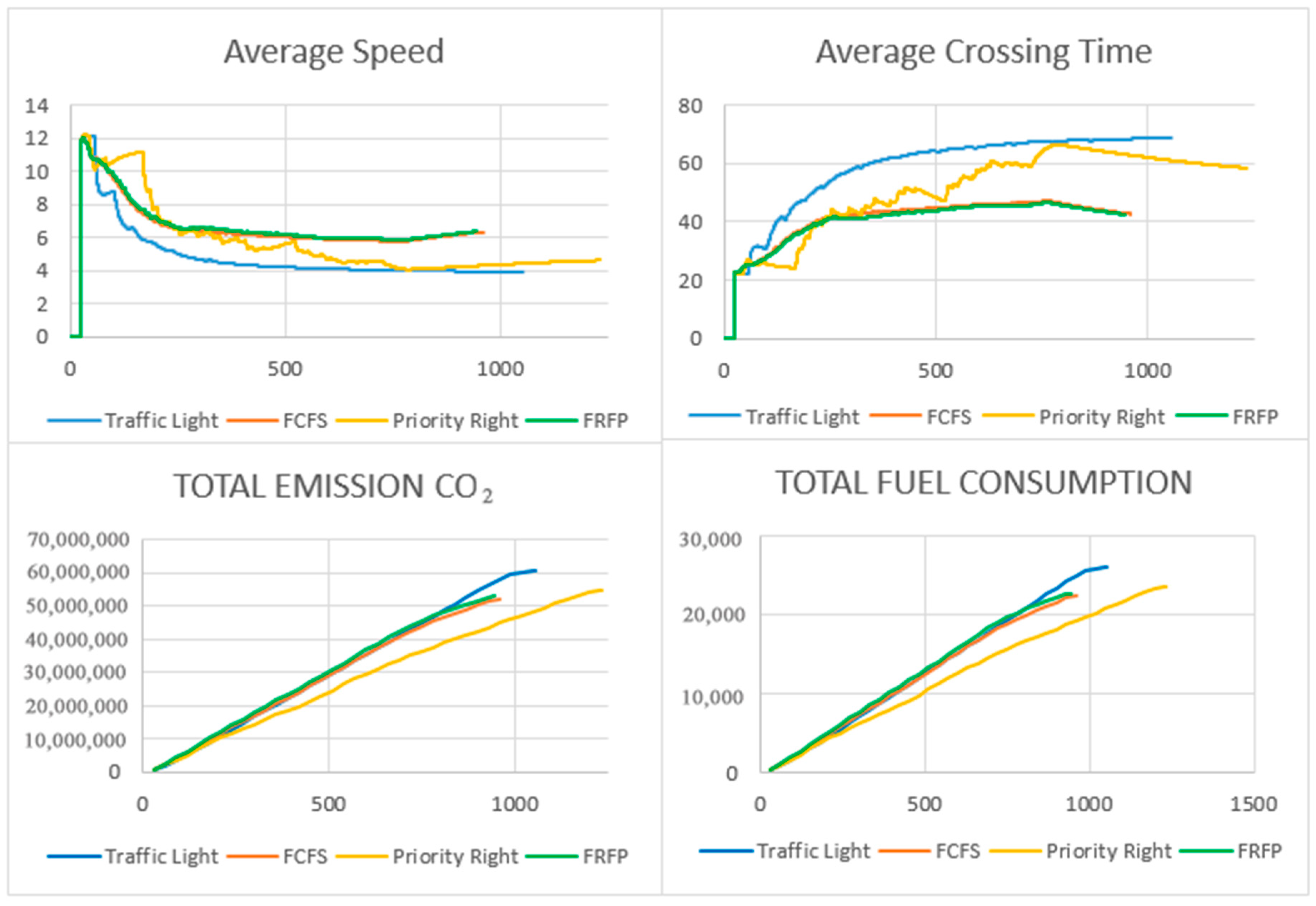
For the two-lane intersection (Figure 12) the two FCFS and FRFP sets have very similar performances. The simulation was performed generating a flow of vehicles equal to about 1950 per hour in a first case and equal to about 3450 per hour in a second case. The following algorithms have been compared (Figure 13): FCFS, FRFP, traffic light, priority right. For congestions so high, it is normal not to notice any difference between the FCFS and FRFP algorithms, in fact the vehicles will be so crowded that the algorithms will behave in an almost equivalent way. The advantage over conventional systems is noticeable. In fact in this case we see an increase in average speed of around 143% and a reduction in emissions of about 60%.

Case 1 (1950 Vehicles/H): The following table (

Table 1. Intersection 2 lanes 1950 Vehicles/h.

	AVERAGE SPEED [m/sec]	Increase FRFP Vs Algorithm	AVERAGE CROSSING TIME [sec]	Reduction FRFP Vs Algorithm
Traffic Light	4.49	143.8%	57.26	60.1%
Priority R.	6.07	80.3%	42.84	46.7%
FCFS	4.49	0.1%	22.87	0.1%
FRFP	6.07	0.0%	22.86	0.0%
	EMISSION CO2 [mg]	Reduction FRFP Vs Algorithm	FUEL CONSUMPTION [mL]	Reduction FRFP Vs Algorithm
Traffic Light	68,344,189	37.2%	29,379	37.2%
Priority R.	60,673,945	29.3%	26,082	29.3%
FCFS	42,990,996	0.2%	18,480	0.2%
FRFP	42,900,123	0.0%	18,441	0.0%

) shows the considerable advantages of the developed system compared to traditional intersection management systems. As we can see from the results, the developed algorithm (FRFP) presents considerably higher performances comparing it to the classic traffic light system and they are not much better than the FCFS system. The FRFP system shows an increase of 143.8% on average speed compared to the traffic light system and 0.1% on the FCFS system. As shown in the table above, it exhibits better performance also in terms of average transit time, emissions and fuel consumption.

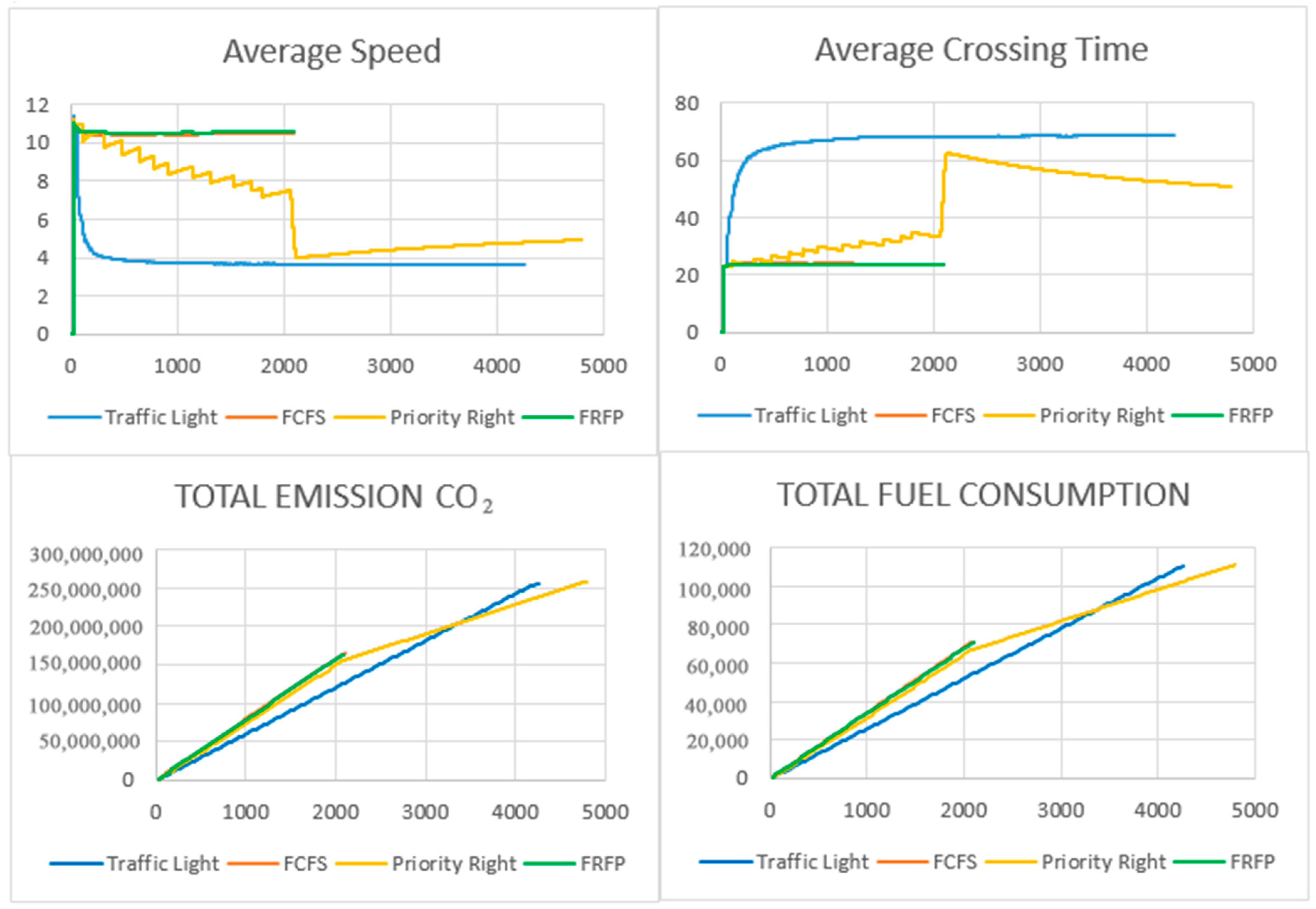
Case 2 (3450 Vehicles/H)): Also in this case, with a congestion considerably higher than the previous case, as we can see from the results, the algorithm developed (FRFS) presents considerably higher performances comparing it to the classic traffic light system and they are little better than the FCFS system (Figure 14). The FRFS system shows (

Table 2. Intersection 2 lanes 3450 Vehicles/H.

	AVERAGE SPEED [m/sec]	Increase FRFP Vs Algorithm	AVERAGE CROSSING TIME [sec]	Reduction FRFP Vs Algorithm
Traffic Light	3.83	175.3%	66.41	64.3%
Priority R.	6.35	66.2%	44.01	46.1%
FCFS	10.46	0.8%	23.90	0.8%
FRFP	10.54	0.0%	23.71	0.0%
	EMISSION CO2 [mg]	Reduction FRFP Vs Algorithm	FUEL CONSUMPTION [mL]	Reduction FRFP Vs Algorithm
Traffic Light	258,094,493	36.7%	110,946	36.7%
Priority R.	255,912,571	36.2%	110,008	36.2%
FCFS	164,778,985	0.9%	70,831	0.9%
FRFP	163,263,697	0.0%	70,180	0.0%

) a 173.3% increase in average speed compared to the traffic light system and 0.8% compared to the FCFS system. As shown in the table above, it exhibits better performance also in terms of average transit time, emissions and fuel consumption.

Intersection type 2 (on-ramp) (Figure 15):

The on-ramp system (Figure 15) has been simulated by inserting around 500 vehicles for an equivalence of 1773 vehicles/h. Also in this case the algorithm is very performing compared to traditional systems but very similar to the FCFS system (Figure 16).

As for the two-lane intersections, for congestions so high, it is normal not to notice any difference between the FCFS and FRFP algorithms, in fact the vehicles will be so crowded that the algorithms will behave in an almost equivalent way. In this case we see an increase in average speed (

Table 3. Intersection on-ramp 1773 Vehicles/H.

	AVERAGE SPEED [m/sec]	Increase FRFP Vs Algorithm	AVERAGE CROSSING TIME [sec]	Reduction FRFP Vs Algorithm
Traffic Light	4.91	38.8%	59.39	31.0%
Priority R.	5.96	14.2%	50.37	18.6%
FCFS	6.7	1.7%	41.73	1.7%
FRFP	6.81	0.0%	41.00	0.0%
	EMISSION CO2 [mg]	Reduction FRFP Vs Algorithm	FUEL CONSUMPTION [mL]	Reduction FRFP Vs Algorithm
Traffic Light	60,569,184	12.6%	26,037	12.6%
Priority R.	54,780,609	3.4%	23,548	3.4%
FCFS	51,981,274	−1.8%	22,345	−1.8%
FRFP	52,912,280	0.0%	22,745	0.0%

) of around 39% and a reduction in emissions of about 12.6% compared to the FCFS system.

Clearly, the variation in the advantages is linked to the type of intersection and the flow of vehicles. This simulation was set by forcing a large number of vehicles on the intersection ramp.

Intersection type 3 (8 lanes) (Figure 17):

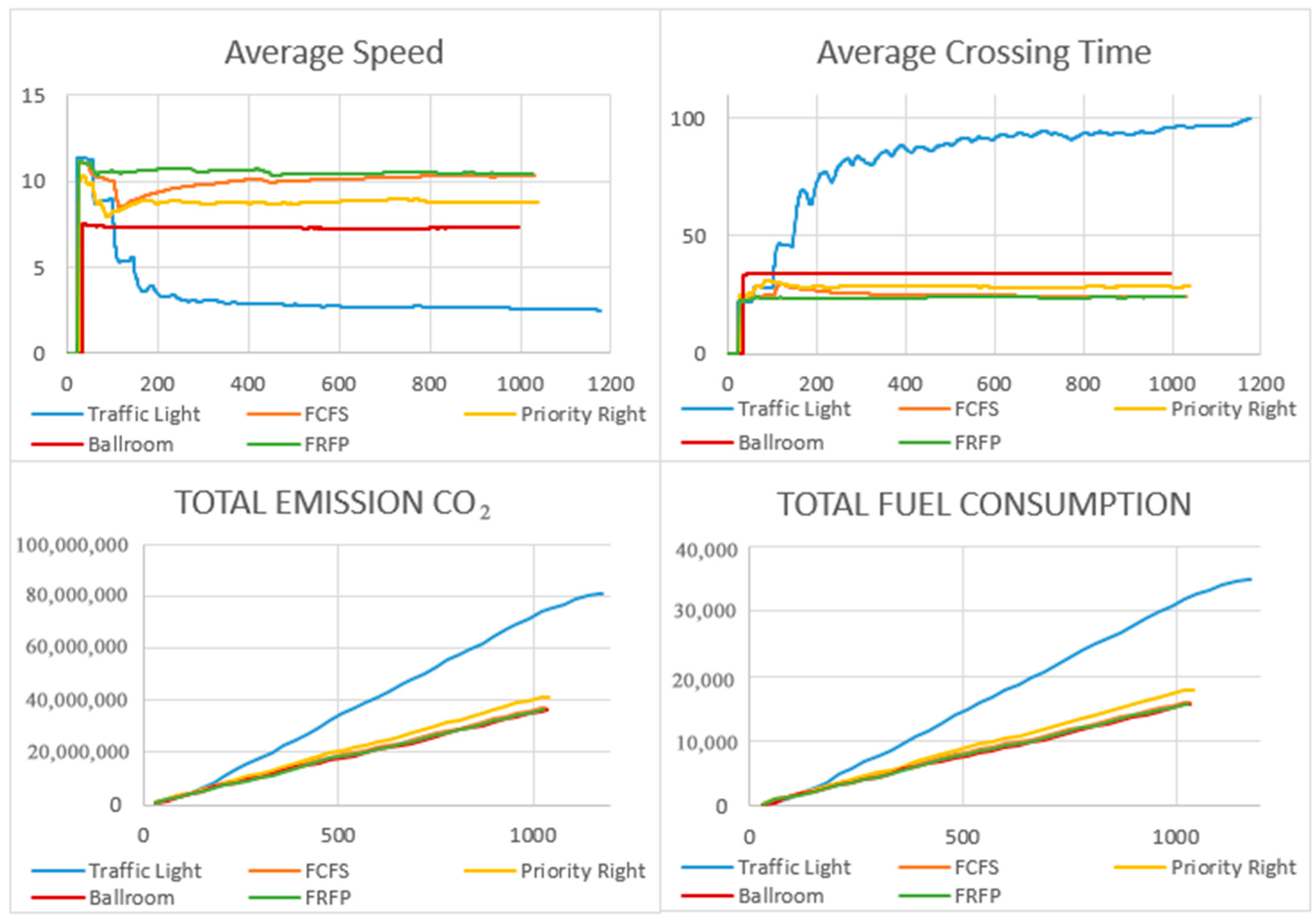
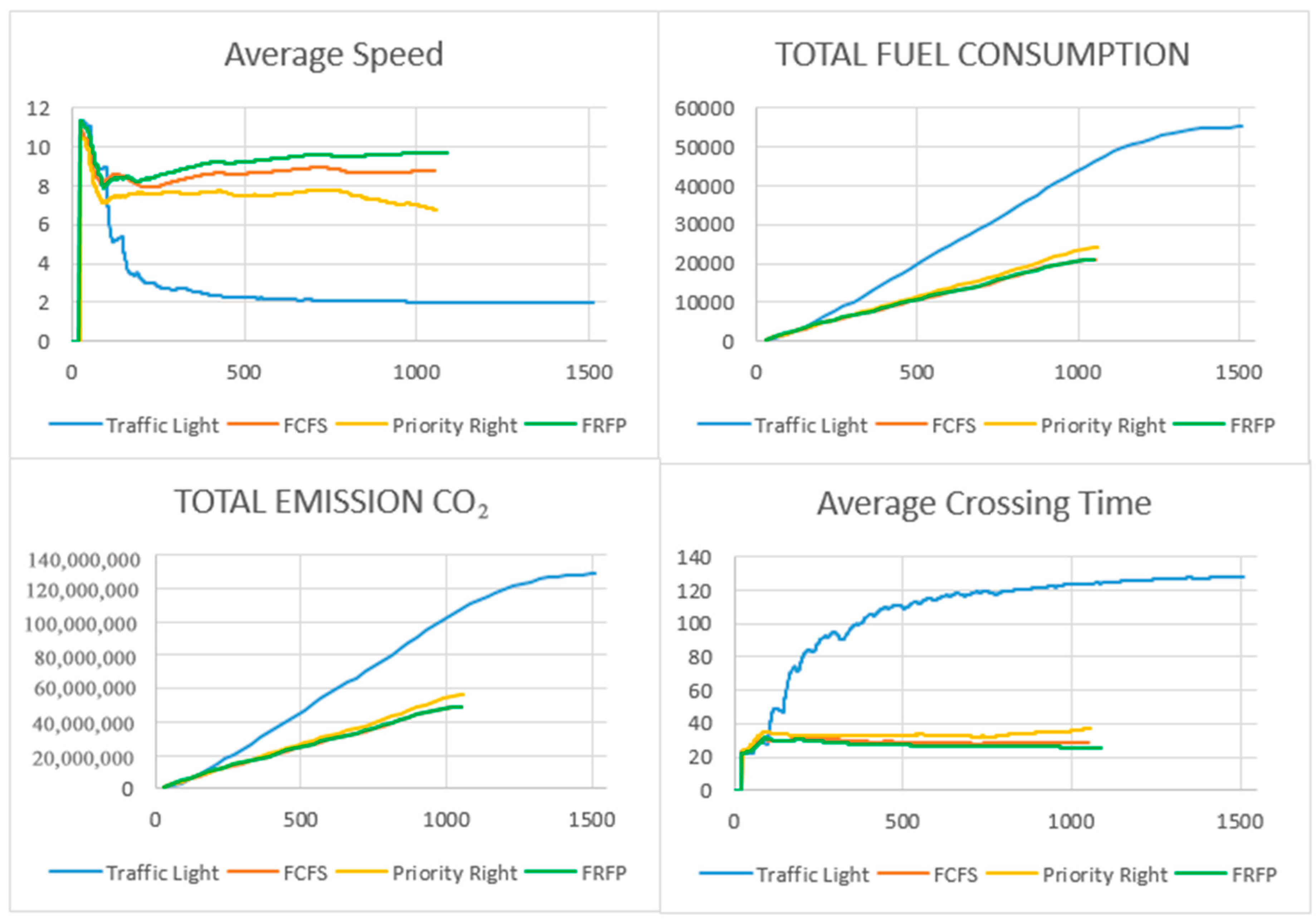
This type of intersection is the most complex (Figure 17). The “ballroom” algorithm, even if compared, has been implemented with considerable application limits. The results obtained provide, in fact, for the “ballroom” algorithm, that all the vehicles involved cannot turn at the intersection, the vehicles can cross the intersection always keeping the same trajectory. Moreover, this algorithm foresees that all vehicles have equal dimensions. In the real application this system, even if in some conditions it has good performances, is not easily applicable both for application limits and for too limited safety margins. The algorithm will no longer be considered in the other tests. This type of intersection has been tested with 4 different levels of congestion: 1640, 1950, 2380, and around 2530. The results are remarkable, showing at best an increase of 22.4% on average speed and a reduction of 14.4% on emissions compared to the FCFS system. The system is all the more effective the more difficult the congestion conditions are. Obviously the results do not improve any more reaching the levels of saturation of the lanes

Case 1 (1640 Vehicles/H): In this case, which is the first case with greater complexity (

Table 4. Intersection 8 lanes 1640 Vehicles/H.

	AVERAGE SPEED [m/sec]	Increase FRFP Vs Algorithm	AVERAGE CROSSING TIME [sec]	Reduction FRFP Vs Algorithm
Traffic Light	3.41	208.9%	83.41	71.6%
BALLROOM	7.3	44.4%	34.26	30.7%
Priority R.	8.8	19.7%	28.42	16.5%
FCFS	10.02	5.2%	25.01	5.1%
FRFP	10.54	0.0%	23.73	0.0%
	EMISSION CO2 [mg]	Reduction FRFP Vs Algorithm	FUEL CONSUMPTION [mL]	Reduction FRFP Vs Algorithm
Traffic Light	81,138,991	55.2%	34,879	55.2%
Priority R.	41,503,757	12.4%	17,841	12.4%
FCFS	36,855,093	1.3%	15,842	1.3%
FRFP	36,371,317	0.0%	15,634	0.0%
BALLROOM	36,168,224	−0.6%	15,548	−0.6%

), we obtain an increase in average speed of 5.2% and a reduction in emissions of 1.3% compared to the FCFS system. The comparison with the traditional traffic light system leads to an increase in the average speed of 208.9%.

From the table the ballroom system results with better performances (Figure 18), but the comparison can not be done on a par with the considerable limits imposed to simulate the algorithm.

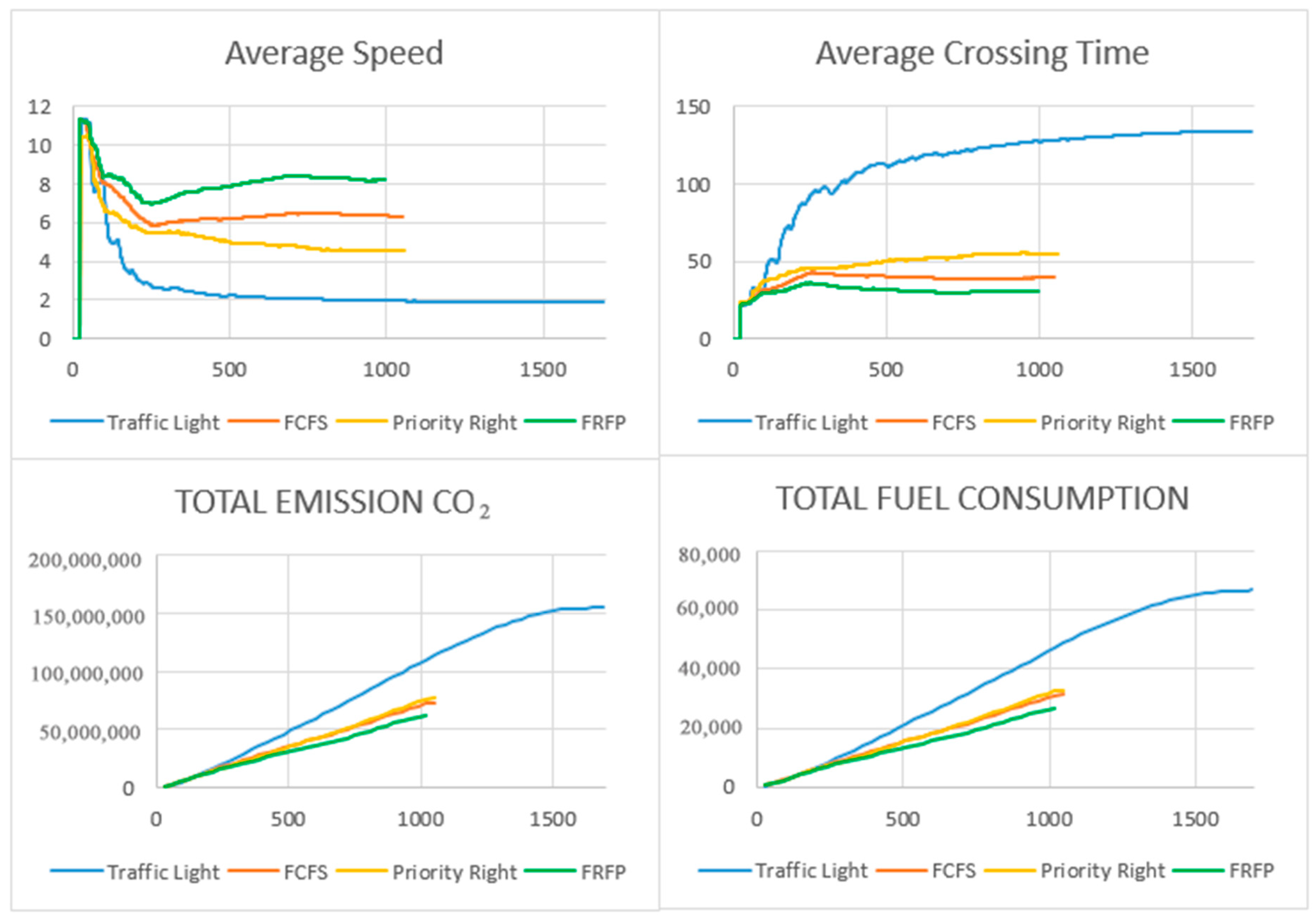
Case 2 (1950 Vehicles/H): As the congestion increases (Figure 19), the performance of the developed system (FRFP) is always more efficient than the other systems compared (

Table 5. Intersection 8 lanes 1950 Vehicles/H.

	AVERAGE SPEED [m/sec]	Increase FRFP Vs Algorithm	AVERAGE CROSSING TIME [sec]	Reduction FRFP Vs Algorithm
Traffic Light	2.73	238.8%	107.86	74.9%
Priority R.	7.56	22.4%	33.19	18.3%
FCFS	8.63	7.3%	29.04	6.6%
FRFP	9.25	0.0%	27.12	0.0%
	EMISSION CO2 [mg]	Reduction FRFP Vs Algorithm	FUEL CONSUMPTION [mL]	Reduction FRFP Vs Algorithm
Traffic Light	128,514,065	61.9%	55,245	61.9%
Priority R.	56,154,276	12.8%	24,138	12.8%
FCFS	49,186,934	0.5%	21,143	0.5%
FRFP	48,961,661	0.0%	21,047	0.0%

).

Case 3 (2380 Vehicles/H): As the congestion increases (Figure 20), the performance of the developed system (FRFP) is always more efficient than the other systems compared (

Table 6. Intersection 8 lanes 2380 Vehicles/H.

	AVERAGE SPEED [m/sec]	Increase FRFP Vs Algorithm	AVERAGE CROSSING TIME [sec]	Reduction FRFP Vs Algorithm
Traffic Light	2.56	217.3%	113.45	72.7%
Priority R.	5.33	52.5%	48.46	36.1%
FCFS	6.64	22.4%	38.26	19.1%
FRFP	8.23	0.0%	30.97	0.0%
	EMISSION CO2 [mg]	Reduction FRFP Vs Algorithm	FUEL CONSUMPTION [mL]	Reduction FRFP Vs Algorithm
Traffic Light	155,409,183	59.7%	66,807	59.7%
Priority R.	77,506,256	19.3%	33,317	19.3%
FCFS	73,131,010	14.4%	31,436	14.4%
FRFP	62,571,993	0.0%	26,897	0.0%

).

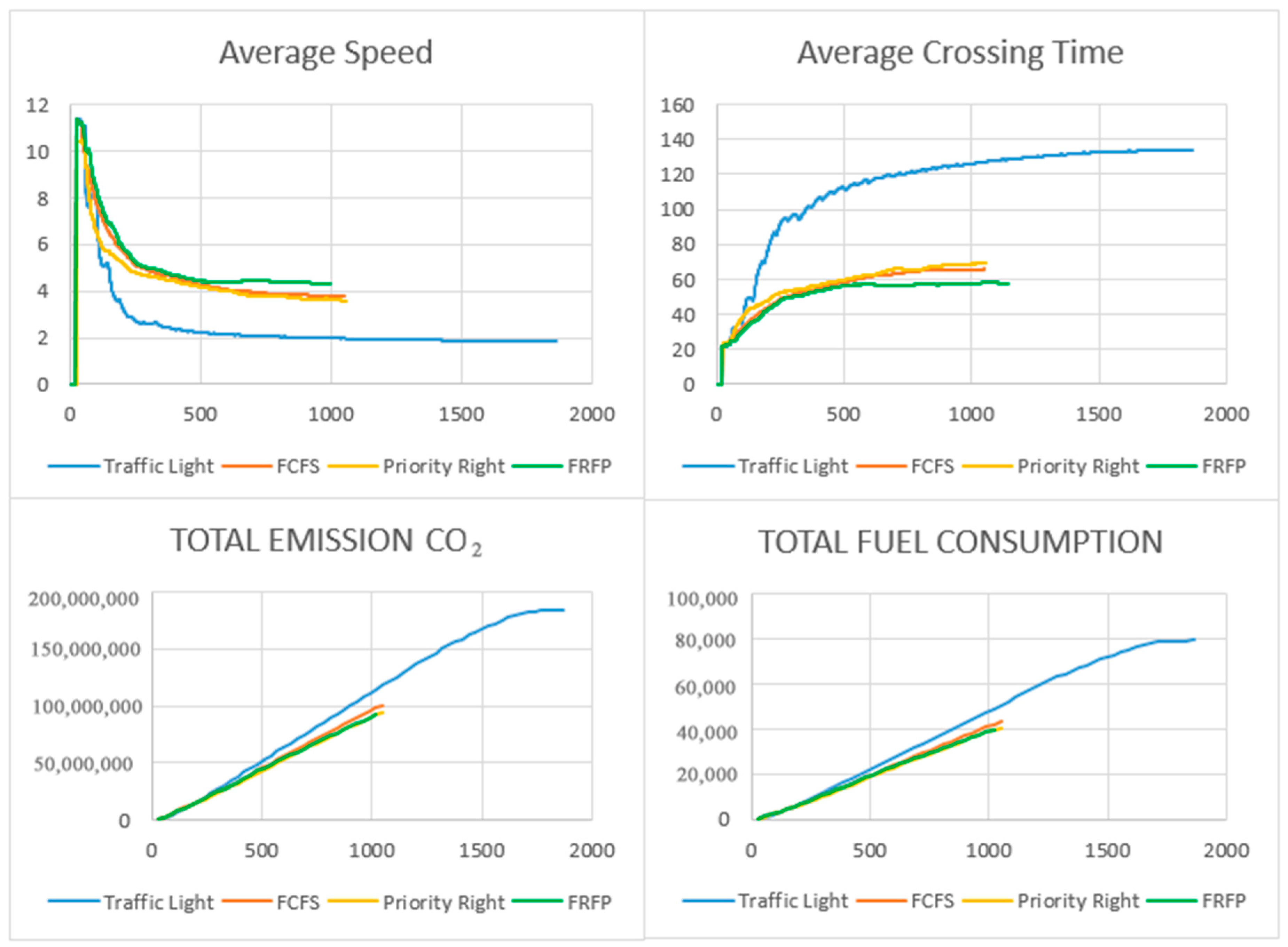
Case 4 (2535 Vehicles/H): In this case we are close to the capacity limit of the lanes, in fact we see a collapse of the performance of the tested algorithms (Figure 21). Also, in this case, our algorithm outperforms the other systems compared (

Table 7. Intersection 8 lanes 2535 Vehicles/H.

	AVERAGE SPEED [m/sec]	Increase FRFP Vs Algorithm	AVERAGE CROSSING TIME [sec]	Reduction FRFP Vs Algorithm
Traffic Light	2.52	104.9%	114.81	55.2%
Priority R.	4.42	16.5%	59.79	13.9%
FCFS	4.77	8.0%	56.17	8.4%
FRFP	5.15	0.0%	51.46	0.0%
	EMISSION CO2 [mg]	Reduction FRFP Vs Algorithm	FUEL CONSUMPTION [mL]	Reduction FRFP Vs Algorithm
Traffic Light	184,500,946	45.9%	79,312	45.9%
Priority R.	107,698,980	7.4%	46,296	7.4%
FCFS	101,270,765	1.5%	43,533	1.5%
FRFP	99,760,467	0.0%	26,897	0.0%

).

In the best case, we have an increase in average speed, with a consequent reduction in average travel time equal to about 240% compared to the classic traffic light system and about 22% compared to the FCFS system. In the worst case the percentages are lowered by about 105% and 5% respectively.

Intersection type 4 (roudabout) (Figure 22):

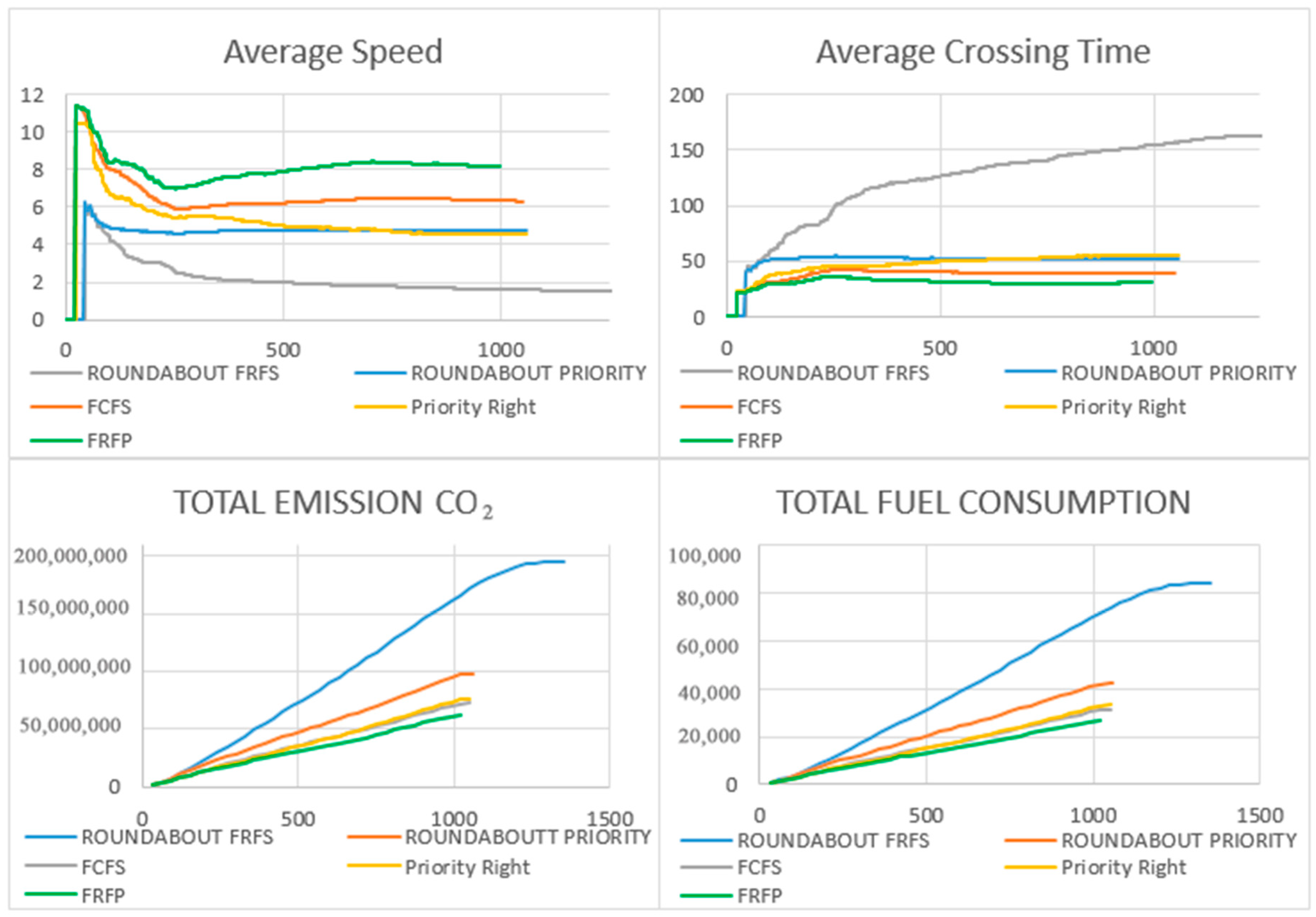
The comparison between the intersection and the roundabout highlights (Figure 22) how in an automatic driving approach the roundabout is much less efficient compared to a classic crossing. In addition, the management of the roundabout is certainly more effective based on priority. Speeding up the entry of vehicles through other systems congested the roundabout and slows down the system.

In the figures below (Figure 23) and in the following tables (

Table 8. Intersection 8 lanes Vs Roundabout 2378 Vehicles/H.

	AVERAGE SPEED [m/sec]	Increase FRFP Vs Algorithm	AVERAGE CROSSING TIME [sec]	Reduction FRFP Vs Algorithm
ROUND FRFP	2.11	285.5%	130.4	76.2%
ROUND PRIORITY	4.78	70.1%	52.34	40.8%
PRIORITY R. 8 lanes	5.33	52.5%	48.46	36.1%
FCFS 8 lanes	6.64	22.4%	38.26	19.%
FRFP 8 lanes	8.13	0.0%	30.97	0.0%
	EMISSION CO2 [mg]	Reduction FRFP Vs Algorithm	FUEL CONSUMPTION [mL]	Reduction FRFP Vs Algorithm
ROUND FRFP	195,903,582	68.1%	84,213	68.1%
ROUND PRIORITY	97,958,974	36.1%	42,108	36.1%
PRIORITY R. 8 lanes	77,506,256	19.3%	33,317	19.3%
FCFS 8 lanes	73,131,010	14.4%	31,436	14.4%
FRFP 8 lanes	62,571,993	0.0%	26,897	0.0%

), we compare our algorithm (FRFP) and the same system by applying the right priority. The right-priority system is more effective than any algorithm tested. The same graphs show another interesting comparison. In the same traffic conditions, the roundabout system is compared to the eight-lane intersection. In particular, it is compared to the right-priority algorithms, FCFS, and FRFP. As is evident from the graphs and the tables that follow, roundabouts in the presence of self-driving vehicles without driver are not effective with characteristics significantly lower than the classic road intersections.

5. Conclusions

In this paper, a new algorithm for the management of road intersections is developed in the exclusive presence of automatically guided vehicles. The proposed method, which can be used in any type of intersection, is simulated and compared with other state-of-the-art algorithms in two lanes, eight lanes, on-ramp, and roundabout intersections. The vehicles involved are free to go straight or turn at the intersection. The entire intersection area is considered as a safety area that can be occupied by only one vehicle at a time. The aforementioned area can also be divided into cells. The proposed system does not necessarily require an intersection operator but is based on vehicle-to-vehicle communications (V2V). The results obtained are very promising. In the best case, which coincides with one of the most critical cases (eight-lane crossing), we obtain an average speed increase equal to 22.4% compared to the FCFS system and 217.3% compared to the classic traffic light system; a reduction in the average crossing time of 19.1% compared to the FCFS system and 72.7% compared to the classic traffic light system; a reduction in CO₂ emissions and fuel consumption of 14.4% compared to the FCFS system and 59.7% compared to the classic traffic light system. The system developed, as shown by the results obtained from the simulations, presents excellent performance in all the types of intersections examined. Another important result was obtained in the analysis of roundabouts in systems with only the presence of self-driving vehicles without a driver. In fact, in this case, it is true that roundabouts are less effective than the classic road crossings, and that through the proposed system (FRFP), both travel times, CO₂ emissions, and consumption are considerably reduced. The system can be further improved by applying V2IC communication systems to perform a pre-setting already at long distances.

6. Future Work

The evolution of this work can be the integration of pedestrians into the system and the analysis of a pre-regulation by means of V2IIC communication. This type of communication could also facilitate the routing of vehicles both according to different environmental parameters for a reduction of emissions and to facilitate the pedestrian crossing in cases with a high presence of pedestrians. It is also useful to analyze a certain percentage of non-automatic vehicles.