Sampling-Based Motion Planning for Free-Floating Space Robot without Inverse Kinematics

Abstract

Motion planning is one of the most important technologies for free-floating space robots (FFSRs) to increase operation safety and autonomy in orbit. As a nonholonomic system, a first-order differential relationship exists between the joint angle and the base attitude of the space robot, which makes it pretty challenging to implement the relevant motion planning. Meanwhile, the existing planning framework must solve inverse kinematics for goal configuration and has the limitation that the goal configuration and the initial configuration may not be in the same connected domain. Thus, faced with these questions, this paper investigates a novel motion planning algorithm based on rapidly-exploring random trees (RRTs) for an FFSR from an initial configuration to a goal end-effector (EE) pose. In a motion planning algorithm designed to deal with differential constraints and restrict base attitude disturbance, two control-based local planners are proposed, respectively, for random configuration guiding growth and goal EE pose-guiding growth of the tree. The former can ensure the effective exploration of the configuration space, and the latter can reduce the possibility of occurrence of singularity while ensuring the fast convergence of the algorithm and no violation of the attitude constraints. Compared with the existing works, it does not require the inverse kinematics to be solved while the planning task is completed and the attitude constraint is preserved. The simulation results verify the effectiveness of the algorithm.

1. Introduction

Free-floating space robots (FFSRs) are composed of a manipulator and a base spacecraft. The base attitude and position control system is closed, and the base attitude is adjusted by joint motion. This mechanism has the advantages of saving fuel and prolonging system life. Therefore, FFSRs are widely employed for on-orbit services [1]. Motion planning is one of the fundamental technologies for FFSRs to achieve autonomy [2]. For a manipulator, it is required that the joint motion is planned so that the end-effector (EE) moves from the initial pose to the goal pose. The general motion planning framework for a manipulator consists of three steps [3]. First, inverse kinematics is used to map the goal EE’s pose to a goal configuration. For a fixed base manipulator, the configuration space is the joint space, and the configuration space for FFSRs includes joint space and base attitude space. Then, the path from the initial configuration to the goal configuration is generated through a sampling-based planning algorithm or other algorithms. Finally, the generated path points are interpolated to obtain the trajectory. This framework works well for a base-fixed manipulator, while it is not suitable for FFSRs. FFSRs have nonholonomic characteristics, and a first-order differential relationship exists between joint angles and base attitude. In addition, this planning framework still has the following disadvantages. First, it is difficult to obtain the analytical inverse kinematics resolution. Second, the obtained goal configuration and the initial configuration may not be in the same connected domain.

For the motion planning of an FFSR, scholars have studied the steering problem at an early stage, where obstacles were not considered in their methods. The FFSR can move from an initial configuration to a goal configuration by using action series generated by these steering methods. Based on the virtual manipulator (VM) model [4], Vafa, Z. et al. developed the self-correcting motions method [4] and the disturbance map (DM) method [5]. In the self-correcting motions method, periodic joint motions are used to adjust base attitude. In the DM method, the joint space is divided into grid points, and the joint motion directions with the largest and smallest base attitude disturbances are drawn at each point. Based on this, the path with less base attitude disturbance is selected. Nakamura, Y. and Mukherjee, R. [6] used Lie brackets and the Frobenius theorem to discuss the nonholonomic characteristics of FFSRs and proposed the bi-directional approach using the Lyapunov function. In this method, the base attitude and the joint position are simultaneously controlled by using only the motion of joints. Fernandes, C. et al. [7] proved that the cat-falling problem is equivalent to the nonlinear controllability problem. Then, they proposed the steering method of coupled rigid bodies and used this method to control the base of an FFSR. The above methods emphasize the nonholonomic characteristics of FFSRs. Joint motion is used to manipulate the base attitude in these methods. However, obstacles are not considered, and they did not discuss the situation where the initial configuration and the goal configuration are not in the same connected domain.

The second method is to convert the motion planning of an FFSR into a nonlinear optimization problem through direct and indirect methods. Yamada, K. [8] used the variational method to plan the joint path, and the base attitude can be arbitrarily changed in this method. Suzuki, T. and Nakamura, Y. [9] extended Yamada, K.’s method, and the spiral perturbation was used to approximate joint motions. The pose of EE and the base attitude can be arbitrarily changed by only controlling 6-degree-of-freedom joints in the method proposed by Suzuki, T. and Nakamura, Y. In 2010, Lampariello, R. [10] studied the motion planning problem of capturing a spin target for space robots, and the problem was converted into a nonlinear optimization problem. The success of this optimization-based approach for robotic motion planning [11,12,13] inspired scholars to apply this idea to the motion planning of space robots. Misra, G. et al. [14] studied the motion planning problem of a space robot with task constraints in 2017, and the problem was constructed as a convex quadratic programming problem. Inspired by Schulman, J. et al. [11], Virgili-Llop, J. et al. [15] used convex optimization to develop a motion planning method for a space robot to capture a spin target. This method divides the process of capturing the spin target into the whole system transfer phase and the internal reconstruction phase. Therefore, the whole planning process is divided into two suboptimization problems. However, the aforementioned methods are not aimed at a space robot working in free-floating mode. Due to the advancement of nonlinear optimization technology and the promotion of various open-source optimization tools, regarding robotic motion planning problem as an optimal control problem is receiving more and more attention. However, this method can lead to local minimum results.

The last type of method is specially developed for FFSRs and is called the approach based on direct kinematics (ABDK). Polynomials with unknown coefficients are first used to parameterize joint trajectories, and then the initial and final configurations of FFSRs are used to eliminate some unknown coefficients of polynomials. The remaining unknown parameters are finally regarded as parameters to be optimized. The objective function is set as a base attitude disturbance at the final time, and the motion planning problem is converted into a nonlinear optimization problem. The nonlinear optimization problem can be solved using particle swarm optimization [16], genetic algorithm [17], differential evolution algorithm [18], and other metaheuristic algorithms. Optimization-based approach for robotic motion planning (OPMP), such as CHOMP (covariant Hamiltonian optimization for motion planning) [12] and STOMP (stochastic trajectory optimization for motion planning) [13], also convert motion planning problems into nonlinear optimization problems, but they are different from ABDK. The trajectory is discretized into N-1 segments in OPMP, and then positions of N discrete points are selected as the variables to be optimized. Therefore, the trajectory shape is easy to be controlled by optimizing N discrete points, and the no-collisions constraint is also easily formulated. Finally, in OPMP, the optimization problem is solved using fast convergence optimization methods based on gradient or the Hessian matrix. In ABDK for FFSRs, the trajectory is parameterized, with only the initial and final configurations, so the trajectory shape cannot be controlled. Finally, ABDK for FFSRs does not consider obstacle avoidance, so the researchers who use this method do not consider whether the initial configuration and the target configuration are in the same connected domain.

Sampling-based motion planners (SBMPs) can efficiently solve the motion planning problem for robots with high degrees-of-freedom (DOF), and local minima can also be avoided in SBMPs. Among existing SBMPs, rapidly exploring random trees (RRTs) are especially suitable for motion planning with differential constraints. Basic RRTs usually take the initial configuration and the goal configuration as input to construct a tree data structure. The initial configuration is selected as the root node, and the goal configuration is used as a heuristic. The tree is grown in the iterative process, and local planning is performed from one selected node of the tree in each iteration; we call this node a node to be extended. During the process of local planning, a guiding point is used to guide the growth of the tree. The guiding point can be a randomly selected configuration or the goal configuration. Goal configuration guiding growth ensures the rapid convergence of the algorithm, while random guiding growth prevents the algorithm from falling into a local minimum. However, this framework also has the following problems. First, it is difficult to obtain an analytical inverse kinematics resolution for a manipulator. Second, the target configuration and the initial configuration may not be in the same connected domain [19]. In order to solve this problem, Weghe, M. V. et al. [20] gave a solution based on the basic framework of RRTs and called this method Jacobian transpose-directed rapidly exploring random trees (JT-RRTs). The goal EE pose was used in goal guiding growth in JT-RRTs. Moreover, in order to deal with local planning in goal guiding growth, the error of the EE pose was mapped to the configuration space through the transpose of the Jacobian matrix. The JT-RRTs method is very powerful for the motion planning of a base-fixed manipulator, but it is not enough for the motion planning of FFSRs for the following two reasons. First, FFSR is a nonholonomic system with differential constraints, while JT-RRTs can only give a geometric path. Second, the local planning approach for goal guiding growth in JT-RRTs cannot ensure that there is no violation of base attitude constraints.

Faced with these questions, this paper investigates a novel motion planning method based on RRT for an FFSR from an initial configuration to a goal EE pose. The main problem in motion planning of FFSRs is that it is a system with differential constraints, and the base attitude disturbance must be restricted in the final trajectory planned for it. The final trajectory is composed of several locally planned trajectories when using RRTs for motion planning. In order to meet the above requirements, the following specific local planners are designed.

• For random configuration guiding growth, three local planning schemes can be found for the motion planning of robots with differential constraints. The first scheme selects a random action and integrates for a certain period of time from the node to be extended with this action. The selected action is treated as a constant during the integration. The second scheme solves a two-point boundary value problem. The third scheme gives several actions that are reasonably distributed in the action space and then integrates for a certain period of time from the node to be extended with these actions. The selected actions are also treated as constants during the integration. Finally, the action with an integration result that is closest to the guiding point is chosen. Obviously, the first and third schemes are not convenient for considering the base disturbance, and the second scheme is time-consuming. This paper proposes a control-based local planner for random configuration guiding growth of the tree. Actions are selected according to the error between the guiding point and the point to be expanded in this local planner. This local planner can achieve rapid local planning and restrict the base attitude disturbance.
• For goal EE pose guiding growth, the requirements of base attitude disturbance cannot be omitted. For JT-RRTs, only the error of EE needs to be considered in the local planning of goal EE pose guiding growth. In JT-RRTs, the DOF of the EE pose is 6, while the DOF of joint space is 7, which is redundant relative to the former. However, the local planner for FFSRs must deal with not only the error of EE but also the base disturbance, which has another 3 DOF. This paper proposes a control-based goal EE pose guiding local planner (CB-EEPG-LP) for goal EE pose guiding growth. Different from the local planner in JT-RRTs, CB-EEPG-LP can not only guide the tree toward the goal pose but also coordinate the base attitude when necessary. The actions are designed based on two kinds of errors: the first is the error between the goal EE pose and the EE pose corresponding to the configuration to be expanded, and the second is the error between the reference goal base attitude and the attitude corresponding to the configuration to be expanded. The proposed local planner can complete the goal EE pose guiding growth and avoid singularity as much as possible. Moreover, the base attitude disturbance meets the requirements.

The rest of this paper is organized as follows. Motion equations for FFSRs are presented in Section 2. The proposed motion planning algorithm is introduced in Section 3. In Section 4, two scenarios of numerical simulations are carried out to validate the proposed motion planning algorithm. Section 5 concludes the work.

2. Motion Equations of an FFSR

The motion model is fundamental for the motion planning and control of a robot, and this part establishes the motion equation of FFSRs. In this paper, RRTs are used for the motion planning of FFSRs, which uses a random configuration and the goal EE pose to guide the growth of the tree. We call them random configuration guiding growth (RC-GG) and goal EE pose guiding growth (GEE-GG), respectively. The Jacobian matrix related to the state transition is needed to perform local planning in RC-GG. For local planning of GEE-GG, the generalized Jacobian matrix and the Jacobian matrix related to base attitude will be used, of which the former is used to reduce the end error and the latter is used to adjust the attitude of the base. In order to detect whether an FFSR is in collision, a method is proposed to calculate the centroid position of each rigid body of the FFSR.

The derivation of the above equations is based on the geometric relations between links. However, the special characteristic also needs to be considered when establishing the motion equations of FFSRs. Therefore, this section also gives the linear momentum and angular momentum conservation equations in velocity form and the linear momentum conservation equation in position form. The symbol definition is the same as that of general space robotics literature.

2.1. Basic Equations of Motion in Position Form

The basic equations of motion in position form only considers that the geometric relationship between rigid bodies belongs to the FFSR. From the base to the $n^{th}$ link, the attitude transformation matrix between the fixed coordinate systems of adjacent rigid bodies is ${}^{i-1}{\mathit{R}}_i,i=1,2,\dots ,n$, and it is a function of the joint angle: ${}^{i-1}{\mathit{R}}_i={\mathit{f}}_1\left({\theta }_i\right),i=1,2,\dots ,n$. ${}^I{\mathit{R}}_0$ denotes the attitude transformation matrix from the base coordinate system to the inertial coordinate system. It is a function of the base attitude angle ${}^I{\mathit{R}}_0={\mathit{f}}_2\left({\mathit{\Psi }}_b\right)$. Through the chain transformation, the attitude of each rigid body can be obtained, and it can be described by the attitude transformation matrix from the coordinate system of each rigid body to the inertial coordinate system:

$${}^I{\mathit{R}}_i{=}^I{\mathit{R}}_0{}^0{\mathit{R}}_1{}^1{\mathit{R}}_2{\dots }^{i-1}{\mathit{R}}_i$$

(1)

As mentioned before, the configuration space for FFSRs includes joint space and base attitude space. Therefore, the configuration parameter of FFSRs includes $\mathit{\Theta }={\left[\begin{array}{cccc}{\theta }_1& {\theta }_2& \dots & {\theta }_n\end{array}\right]}^T$ and ${\mathit{\Psi }}_b$. The above formula reflects the mapping relationship between the attitude of each rigid body and the configuration parameter. Let ${\mathit{r}}_0$ denotes the centroid position vector of the base; the centroid position vector of each rigid body can be obtained recursively from ${\mathit{r}}_0$:

$${\mathit{r}}_i={\mathit{r}}_0+{\mathit{b}}_0+{\displaystyle \sum _{j=1}^{i-1}\left({\mathit{a}}_j+{\mathit{b}}_j\right)}+{\mathit{a}}_i,i=1,2,\dots ,n$$

(2)

The position vector of the end of each rigid body is still recursively obtained from ${\mathit{r}}_0$:

$${\mathit{p}}_i={\mathit{r}}_0+{\mathit{b}}_0+{\displaystyle \sum _{j=1}^i\left({\mathit{a}}_j+{\mathit{b}}_j\right)},i=0,1,2,\dots ,n$$

(3)

Vectors can be added only if they are expressed in the same coordinate system. Therefore, the above vectors must be expressed in the inertial coordinate system when performing the calculation. Representations of ${\mathit{b}}_i,{\mathit{a}}_i$ in the inertial space are denoted as ${}^I\mathit{b}{}_i,{}^I\mathit{a}{}_i$. ${}^I\mathit{b}{}_i,{}^I\mathit{a}{}_i$, depending on the configuration parameter, so in order to calculate ${\mathit{r}}_i$ and ${\mathit{p}}_i$, ${\mathit{r}}_0$ and the configuration parameter must be known. In Section 2.3, we will show how to calculate ${\mathit{r}}_0$ when the configuration parameter is given.

2.2. Basic Motion Equation and Momentum Conservation Equation in Velocity Form, Jacobian Matrix

The momentum conservation equation in velocity form is employed to derive the Jacobian matrix related to state transition, the generalized Jacobian matrix, and the Jacobian matrix related to base attitude. In order to obtain the momentum conservation equation in velocity form, the velocity equation of each link must be given. The angular velocity of each link is

$${\mathit{\omega }}_i={\mathit{\omega }}_0+{\displaystyle \sum _{j=1}^i{\mathit{k}}_j{\dot{\theta }}_j},i=1,2,\dots ,n$$

(4)

The linear velocity of the mass center of each link is

$${\mathit{v}}_i={\dot{\mathit{r}}}_i={\mathit{v}}_0+{\mathit{\omega }}_0\times \left({\mathit{r}}_i-{\mathit{r}}_0\right)+{\displaystyle \sum _{j=1}^i\left[{\mathit{k}}_j\times \left({\mathit{r}}_i-{\mathit{p}}_j\right)\right]{\dot{\theta }}_j},i=1,2,\dots ,n$$

(5)

In addition, the linear velocity of EE is

$${\mathit{v}}_e={\dot{\mathit{p}}}_e={\mathit{v}}_0+{\mathit{\omega }}_0\times \left({\mathit{p}}_e-{\mathit{r}}_0\right)+{\displaystyle \sum _{j=1}^n\left[{\mathit{k}}_j\times \left({\mathit{p}}_e-{\mathit{p}}_j\right)\right]{\dot{\theta }}_j}$$

(6)

According to Equations (4) and (6), the linear velocity and angular velocity of the EE can be obtained. The matrix form is

$$\left[\begin{array}{c}{\mathit{v}}_e\\ {\mathit{\omega }}_e\end{array}\right]={\mathit{J}}_b\left[\begin{array}{c}{\mathit{v}}_0\\ {\mathit{\omega }}_0\end{array}\right]+{\mathit{J}}_m\dot{\mathit{\Theta }}$$

(7)

where ${\mathit{J}}_b$ and ${\mathit{J}}_m$ are the Jacobian matrixes relative to the base and the joint angle, respectively.

$${\mathit{J}}_b=\left[\begin{array}{cc}{\mathit{E}}_{3\times 3}& -{\tilde{\mathit{p}}}_{0e}\\ {\mathit{0}}_{3\times 3}& {\mathit{E}}_{3\times 3}\end{array}\right],{\mathit{p}}_{0e}={\mathit{p}}_e-{\mathit{r}}_{0e},{\mathit{J}}_m=\left[\begin{array}{cccc}\begin{array}{c}{\mathit{k}}_1\times \left({\mathit{p}}_e-{\mathit{p}}_1\right)\\ {\mathit{k}}_1\end{array}& \begin{array}{c}{\mathit{k}}_2\times \left({\mathit{p}}_e-{\mathit{p}}_2\right)\\ {\mathit{k}}_2\end{array}& \dots & \begin{array}{c}{\mathit{k}}_n\times \left({\mathit{p}}_e-{\mathit{p}}_n\right)\\ {\mathit{k}}_1\end{array}\end{array}\right]$$

Given two vectors $\mathit{v}={\left[\begin{array}{ccc}x& y& z\end{array}\right]}^T$ and $\mathit{w}$, the cross-product operator is defined as follows:

$$\tilde{\mathit{v}}=\left[\begin{array}{ccc}0& -z& y\\ z& 0& -x\\ -y& x& 0\end{array}\right],\mathit{v}\times \mathit{w}=\tilde{\mathit{v}}\mathit{w}$$

The linear momentum is

$$\mathit{P}=m_0{\dot{\mathit{v}}}_0+{\displaystyle \sum _{i=1}^n\left(m_i{\dot{\mathit{v}}}_i\right)}=m_0{\dot{\mathit{r}}}_0+{\displaystyle \sum _{i=1}^n\left(m_i{\dot{\mathit{r}}}_i\right)}$$

(8)

Additionally, the angular momentum is

$$\mathit{L}={\displaystyle \sum _{i=0}^n\left[I_i{\mathit{\omega }}_i+{\mathit{r}}_i\times \left(m_i{\dot{\mathit{v}}}_i\right)\right]}={\displaystyle \sum _{i=0}^n\left[I_i{\mathit{\omega }}_i+{\dot{\mathit{r}}}_i\times \left(m_i{\dot{\mathit{r}}}_i\right)\right]}$$

(9)

Substituting (4) and (5) into the above formulas and sorting them into matrix form, we can get the linear momentum equation:

$$\mathit{P}=\left[\begin{array}{cc}M\mathit{E}& M{\tilde{\mathit{r}}}_{og}{}^T\end{array}\right]\left[\begin{array}{c}{\dot{\mathit{v}}}_0\\ {\omega }_0\end{array}\right]+{\mathit{J}}_{T\mathit{w}}\dot{\mathit{\Theta }}$$

(10)

where

$${\mathit{r}}_{og}={\mathit{r}}_g-{\mathit{r}}_0,{\mathit{J}}_{Tw}={\displaystyle \sum _{i=1}^n\left(m_i{\mathit{J}}_{Ti}\right)}$$

$${\mathit{J}}_{Ti}=\left[\begin{array}{ccccccc}{\mathit{k}}_1\times \left({\mathit{r}}_i-{\mathit{p}}_1\right)& {\mathit{k}}_2\times \left({\mathit{r}}_i-{\mathit{p}}_2\right)& \dots & {\mathit{k}}_i\times \left({\mathit{r}}_i-{\mathit{p}}_i\right)& 0& \dots & 0\end{array}\right]$$

The angular momentum is

$$\mathit{L}=\left[\begin{array}{cc}M{\tilde{\mathit{r}}}_{0g}& {\mathit{H}}_w\end{array}\right]\left[\begin{array}{c}{\dot{\mathit{v}}}_0\\ {\mathit{\omega }}_0\end{array}\right]+{\mathit{H}}_{w\varphi }\dot{\mathit{\Theta }}$$

(11)

where

$${\mathit{H}}_w={\displaystyle \sum _{i=1}^n\left(I_i+m_i{\tilde{\mathit{r}}}_{0i}{}^T{\tilde{\mathit{r}}}_{0i}\right)}+I_0,{\mathit{H}}_{w\varphi }={\displaystyle \sum _{i=1}^n\left(I_i{\mathit{J}}_{Ri}+m_i{\tilde{\mathit{r}}}_{0i}{\mathit{J}}_{Ti}\right),}{\mathit{r}}_{0i}={\mathit{r}}_i-{\mathit{r}}_0$$

$${\mathit{J}}_{Ri}=\left[\begin{array}{ccccccc}{\mathit{k}}_1& {\mathit{k}}_2& \dots & {\mathit{k}}_i& 0& \dots & 0\end{array}\right]$$

Put linear momentum and angular momentum equations together, and we can get

$$\left[\begin{array}{c}\mathit{P}\\ \mathit{L}\end{array}\right]=\left[\begin{array}{c}\begin{array}{cc}M\mathit{E}& M{\tilde{\mathit{r}}}_{og}{}^T\end{array}\\ \begin{array}{cc}M{\tilde{\mathit{r}}}_{0g}& {\mathit{H}}_w\end{array}\end{array}\right]\left[\begin{array}{c}{\dot{\mathit{v}}}_0\\ {\mathit{\omega }}_0\end{array}\right]+\left[\begin{array}{c}{\mathit{J}}_{Tw}\\ {\mathit{H}}_{w\varphi }\end{array}\right]\dot{\mathit{\Theta }}$$

(12)

Let

$${\mathit{H}}_b=\left[\begin{array}{c}\begin{array}{cc}M\mathit{E}& M{\tilde{\mathit{r}}}_{og}{}^T\end{array}\\ \begin{array}{cc}M{\tilde{\mathit{r}}}_{0g}& {\mathit{H}}_w\end{array}\end{array}\right],{\mathit{H}}_m=\left[\begin{array}{c}{\mathit{J}}_{Tw}\\ {\mathit{H}}_{w\varphi }\end{array}\right]$$

where ${\mathit{H}}_b$ is always invertible. The linear momentum and angular momentum of the FFSR are conserved. The initial momentum of the system is assumed to be 0, and the base velocity can be expressed as a linear function of the joint angular velocity:

$$\left[\begin{array}{c}{\dot{\mathit{v}}}_0\\ {\mathit{\omega }}_0\end{array}\right]=-{\mathit{H}}_b{}^{-1}{\mathit{H}}_m\dot{\mathit{\Theta }}={\mathit{H}}_{b\Theta }\dot{\mathit{\Theta }}=\left[\begin{array}{c}{\mathit{H}}_v\\ {\mathit{H}}_{\omega }\end{array}\right]\dot{\mathit{\Theta }}$$

(13)

Combining Equation (7), we can get

$$\left[\begin{array}{c}{\dot{\mathit{v}}}_e\\ {\mathit{\omega }}_e\end{array}\right]={\mathit{J}}_g\dot{\mathit{\Theta }}$$

(14)

where ${\mathit{J}}_g$ is the generalized Jacobian matrix

$${\mathit{J}}_g=-{\mathit{J}}_b{\mathit{H}}_{b\Theta }+{\mathit{J}}_m$$

According to (13), we can also get

$${\mathit{\omega }}_0={\mathit{H}}_{\omega }\dot{\mathit{\Theta }}$$

(15)

where ${\mathit{H}}_{\omega }$ is called the Jacobian matrix related to base attitude. For the rigid body, the relationship between the first derivative of attitude angle and angular velocity is

$$\mathit{\omega }=\mathit{N}{\left[\begin{array}{ccc}\dot{\alpha }& \dot{\beta }& \dot{\gamma }\end{array}\right]}^T$$

(16)

where

$$\mathit{N}=\left[\begin{array}{ccc}1& \tan \left(\beta \right)\ast \sin \left(\alpha \right)& \tan \left(\beta \right)\ast \cos \left(\alpha \right)\\ 0& \cos \left(\alpha \right)& -\sin \left(\beta \right)\\ 0& \sin \left(\alpha \right)/\cos \left(\beta \right)& \cos \left(\alpha \right)/\cos \left(\beta \right)\end{array}\right]$$

$\mathit{\omega }$ is expressed in the coordinate system of the base in Equation (16). Considering the Formulas (15) and (16), the state transition equation of the FFSR can be gotten

$$\left[\begin{array}{c}\dot{\mathit{\Theta }}\\ {\dot{\mathit{\Psi }}}_b\end{array}\right]=\left[\begin{array}{c}{\mathit{E}}_{n\times n}\\ {\mathit{N}}^{-1}{\left({}^I{\mathit{R}}_0\right)}^T\end{array}\right]\dot{\mathit{\Theta }}={\mathit{J}}_x\dot{\mathit{\Theta }}$$

(17)

where ${\mathit{J}}_x$ is the Jacobian matrix related to state transition.

2.3. Calculation of the Location of Feature Points Based on Configuration Parameters

In Section 2.1, basic equations of motion in position form only give the relationship among the centroid position of each rigid body, the position of the base, and the configuration parameter. Therefore, this section will give a method for calculating the base centroid position according to the configuration parameter. Then, the centroid position of each rigid body can be calculated.

The linear momentum conservation of FFSRs is a holonomic constraint. It can be integrated into a positional form. The equation of this integral form is shown in Equation (18). It means that the centroid position of the FFSR, multiplied by the total mass of the system, is equal to the composition of the centroid position of each rigid body multiplied by its mass.

$$M{\mathit{r}}_g=m_0{\mathit{r}}_0+{\displaystyle \sum _{i=1}^n\left(m_i{\mathit{r}}_i\right)}$$

(18)

Bring Equation (2) into the above equation and merge the terms related to the position of the base centroid; we can get

$$M{\mathit{r}}_g=m_0{\mathit{r}}_0+{\displaystyle \sum _{i=1}^n\left(m_i{\mathit{r}}_i\right)}=M{\mathit{r}}_0+{\displaystyle \sum _{i=1}^n\left[m_i\left({\mathit{b}}_0+{\displaystyle \sum _{j=1}^{i-1}\left({\mathit{a}}_j+{\mathit{b}}_j\right)}+{\mathit{a}}_i\right)\right]}$$

(19)

where ${\mathit{r}}_{0i}={\mathit{b}}_0+{\displaystyle \sum _{j=1}^{i-1}\left({\mathit{a}}_j+{\mathit{b}}_j\right)}+{\mathit{a}}_i$ represents the position vector of the centroid of each link relative to the base centroid. Therefore, the above formula can be written as

$$M{\mathit{r}}_g=M{\mathit{r}}_0+{\displaystyle \sum _{i=1}^n\left(m_i{\mathit{r}}_{0i}\right)}$$

(20)

3. Motion Planning Algorithm for FFSRs

In this paper, an RRT-based planning algorithm is designed for FFSRs from an initial configuration to a goal EE pose. In this method, it is not necessary to solve the inverse kinematics to obtain a goal configuration corresponding to the target EE pose. RRTs have a tree data structure, and this data structure includes vertexes and edges. Vertexes are configurations of FFSRs, and edges are local trajectories. In the basic version of RRTs, the tree takes root in the initial configuration and grows in an iterative manner. In each iteration, local planning is performed from one node of the existing tree to generate a new edge and a new node. The algorithm is not terminated until EE reaches the goal or the number of iterations reaches the upper limit.

In the process of local planning, guide points are used to guide the growth of the tree. Guide points can be a random configuration or the goal EE pose, respectively called random configuration guiding growth (RC-GG) and goal EE pose guiding growth (GEE-GG). GEE-GG ensures the rapid convergence of the algorithm. RC-GG guarantees that the algorithm does not fall into a local minimum caused by goal bias. For the RRT algorithm, when using the goal EE pose to guide the growth of the tree, the tree will be directly extended toward the area closer to the goal EE pose, and this will speed up the convergence of the algorithm. However, if the tree only extends directly toward the goal EE pose, sometimes it will be stuck by obstacles or configuration limits, which means that the algorithm falls into a local minimum. When using a random configuration to guide the growth of the tree, the tree will be extended toward the unexplored area, and this will guarantee that the algorithm does not fall into the local minimum caused by GEE-GG. RRTs introduce GEE-GG to a certain probability; otherwise, it will perform random guided growth. That is, in each iteration of RRTs for FFSRs, Line 3 of Algorithm 1 generates a random number within 0~1. If this generated random number is smaller than the constant $p\_g$, the goal EE pose will be selected as the guiding point. Otherwise, a random configuration will be selected as the guiding point. $p\_g$ is a constant between 0 and 1. After selecting the guiding point, according to certain criteria, the node closest to the guide point in the existing tree is selected as the node to be extended. We define this node as ${\mathit{q}}_{Extended}$. Then, the algorithm performs local planning, which can extend the tree toward the guiding point. Collision detection is performed when necessary during local planning. The result of local planning includes a new node and a local trajectory, and they can be added to the tree if they meet some requirements. The pseudo-code of the basic RRT algorithm is shown in Algorithm 1. RC-GG and GEE-GG are subalgorithms of Algorithm 1. RC-GG is used in Line 6 of Algorithm 1 and GEE-GG is used in Line 4 of Algorithm 1. Variables and functions used in Algorithm1 are defined in

Table 1. Variables and functions used in Algorithm 1.

1	Tree	Tree data structure generated by the algorithm
2	V	Vertex of the tree
3	rand()	A function that generates a real number between 0~1
4	q_new	New vertex (configuration) generated by the local planner
5	Local_Traj	Local trajectory generated by the local planner
6	is_Reaching_Goal	A mark indicating whether the goal has been achieved
7	Is_Extend	A mark indicating whether the local planner is successful
8	Tree.Add	A function that adds the generated new node and local trajectory to the tree
9	Tree.V.init(q_I)	Initialize the tree
10	Break	Jump out of the loop

.

Algorithm 1 RRTs for Free-Floating Space Robots
1	Tree.V.init(q_I)
2	for i = 1 to K do
3		If1 rand() < p_g
4			[q_new, Local_Traj, is_Reaching_Goal, Is_Extend] = Extend_Toward_Goal()
5		Else
6			[q_new, Local_Traj, Is_Extend] = Extend_Randomly()
7		End if1
8		If2 Is_Extend = true
9			Tree.Add(q_new, Local_Traj)
11		End if2
12		If3 is_Reaching_Goal = true
13			Break;
14		End if3
15	End for
16	Return tree

3.1. Overview of the Algorithm

For RRTs, the key steps include random sampling, selection of $q_{\mathit{E}xtended}$, local planning, and collision detection. FFSRs are nonholonomic, and their attitude disturbance during the motion cannot exceed a certain range. Therefore, the following problems must be considered and solved when using RRTs for motion planning of FFSRs:

• Random sampling: The configuration space of the FFSR includes the joint space and the space of the base attitude. In order to meet the constraint on base attitude disturbance, it is necessary to limit the sampling space of the base attitude.
• Selection of node to be expanded: Different selection criteria should be considered for GEE-GG and RC-GG when selecting $q_{Extended}$. For the former, the requirement of avoiding larger base disturbances must be considered, so greater weight to the change of base attitude should be provided during the design of the metric. For the latter, the pose change of the EE should be used as the major part of the metric design.
• Local planning: This article designs two types of local planner; one of them is for RC-GG, another is for GEE-GG. The details of these two local planners will be presented in Section 3.2.
• Collision detection: First, in order to test whether a certain configuration is in collision, the centroid position and attitude of each rigid body of the FFSR can be calculated through the related methods in Part 2. Combined with the size parameters of each rigid body, the area occupied by each rigid body in space can be calculated. Then, collision detection can be completed according to the corresponding collision detection algorithm. Second, according to the previous statement, we can see that every local planning scheme has an integration process Each integration will produce a new configuration. The new configuration may change very little from the last configuration because the step length of the integration may be very small. Therefore, it is not necessary to detect the new configuration generated in each integration. In the collision detection module of the planner, a new mechanism is introduced to determine when to perform collision detection. This mechanism will be stated in the local planning section.

3.2. Local Planning

3.2.1. Local Planner for Random Configuration Guiding Growth

The purpose of local planning corresponding to RC-GG is to grow node ${\mathit{q}}_{Extended}$ toward a random guiding configuration to generate local trajectories and new nodes. It is not necessary to reach the random guiding configuration in this local planner. This paper proposes a control-based local planner for RC-GG. The planner runs in an iterative manner. The action in each iteration is designed according to the error between the current configuration and the random guiding configuration. The purpose of this local planning is to extend the tree toward the random guiding configuration instead of reaching the random configuration. Hence, it does not require the convergence of the error between the current configuration and the random guided configuration.

The pseudo-code of this algorithm is shown in Algorithm 2. Variables and functions used in Algorithm 2 are defined in

Table 2. Variables and functions used in Algorithm 2.

1	q_Sample	A randomly sampled configuration
2	Random_Config()	A function that can generate a random configuration
	q_Near	Nearest node in the tree with respect to q_Sample
	q_Present	The current configuration in local planning
3	Last_Checked_Config	Last detected free configuration
4	J_Base	The Jacobian matrix related to base attitude
5	Jacobian_Base()	A function which calculates J_Base
6	J_x	Jacobian matrix related to state transition
7	Dot_Joint/Dot_Base	First derivative of joint angle/base attitude angle
8	Collision_Check_Tresh_Hold	A threshold that indicates the need for collision detection
9	Collision_Check()	A function that used for doing collision checking
10	is_q_Present_over_Tresh_Hold	A mark indicating whether the q_Present meets the limit
11	is_Extend_over_Tresh_hold	A mark indicating whether the extension is far enough from the node to be extended

. The basic principle of the algorithm is as follows. First, a configuration in free configuration space is randomly sampled and the nearest node in the existing space relative to it is found as ${\mathit{q}}_{Extended}$. Second, iterative local planning from ${\mathit{q}}_{Extended}$ is performed, and the iteration continues until the termination condition is reached.

Algorithm 2 Extend_Randomly with Control Based Local Planner
1	q_Sample = Random_Config()
2	q_Near = Nearest_Node(Tree, q_Sample); q_Present = q_Near; Last_Checked_Config = q_Present
3	Shall_End = false
4	While (Shall_End = false)
5		J_Base = Jacobian_Base(q_Present)
6		J_x = [J_Base; eye(n, n)]
7		Delta_q = q_sample − q_present
8		Dot_Joint = pinv(J) * Delta_q; Dot_Base = J_Base * Dot_Joint
9		q_Present = q_Present + [Dot_Base; Dot_Joint] * time_step
10		If Max(q_present − last_Checked_Config) ≥ Collision_Check_Tresh_Hold
11			Is_Collision = Collision_Check(q_Present)
12			last_Checked_Config = q_Present
13		End if
14		Shall_End = is_Collision or is_q_Present_over_Tresh_Hold or is_Extend_over_Tresh_hold
15	End while
16	Is_Extend = if q_Present is far enough from q_Near
17	Return

• Iterative local planning: This process corresponds to Lines 4 to 15 of the pseudo-code. Firstly, the configuration error between ${\mathit{q}}_{Extended}$ and the random configuration is calculated; we defined this error as $\mathsf{\Delta }\mathit{q}$. Secondly, ${\mathit{H}}_{\omega }$ at ${\mathit{q}}_{Extended}$ is calculated, which can be used to obtain the Jacobian matrix ${\mathit{J}}_x$. Through the pseudo-inverse of ${\mathit{J}}_x$, $\mathsf{\Delta }\mathit{q}$ can be mapped to the action space to get joint angular velocity $\dot{\mathit{\Theta }}$

  $$\dot{\mathit{\Theta }}={\mathit{J}}_x{}^{+}\mathsf{\Delta }\mathit{q}$$

  (21)
  $\mathsf{\Delta }\mathit{q}$ can be reduced if the robot moves with $\dot{\mathit{\Theta }}$ at ${\mathit{q}}_{Extended}$. By multiplying $\dot{\mathit{\Theta }}$ by ${\mathit{H}}_{\omega }$, ${\dot{\mathit{\Psi }}}_b$ corresponding to $\dot{\mathit{\Theta }}$ can be obtained. Integrating $\dot{\mathit{\Theta }}$ and ${\dot{\mathit{\Psi }}}_b$ from ${\mathit{q}}_{Extended}$, a new configuration is obtained, and we let this configuration be the next ${\mathit{q}}_{Extended}$. Repeat the above process until the termination condition of local planning is triggered, then exit local planning and return to the new configuration and trajectory.
• Collision detection mechanism: The collision detection mechanism corresponds to Lines 2 and 10–12 of the pseudo-code. In the second line of the algorithm, ${\mathit{q}}_{Extended}$ is selected from the tree and is collision-free. Therefore, ${\mathit{q}}_{Extended}$ is recorded as the last detected free configuration. During iterative local planning, the configuration is gradually changed. The algorithm determines whether collision detection is required, corresponding to the 10th line of the algorithm. The judgment condition is whether the difference between the current configuration and the last detected free configuration reaches a certain threshold. If collision detection is performed after the judgment, the current configuration is recorded as the new last-detected free configuration.
• Termination conditions and return for iterative local planning: (1) The collision detection program detects a collision; (2) the configuration exceeds the limit, that is, the base attitude disturbance exceeds the limit or the joint angle exceeds the range; (3) among the configuration parameters, the maximum expansion value reaches a certain threshold. When any one of these three conditions is met, iterative local planning is terminated. Then, in Line 17 of the pseudo-code, the algorithm tests if the tree is extended far enough from the initial ${\mathit{q}}_{Extended}$. If the generated new configuration is very close to ${\mathit{q}}_{Extended}$, then we let Is_Extend equal to false, and the local planning results will not be added to the tree.
• Remark of parameter setting: In Algorithm 2, there are some parameters that need to be set. (1) Collision_Check_Tresh_Hold: This is a threshold that decides the number of collision detections when running the algorithm. It cannot be set too large or the collision detection will miss some configurations in collision. Additionally, it cannot be set too small or unnecessary collision detection will be carried out and the algorithm will be too slow. This threshold is set at 1 degree in the simulation study, and it worked well. (2) is_Extend_over_Tresh_hold: This is a mark that indicates whether the extend is far enough from the node to be extended. Additionally, it relates to a threshold. This threshold is similar to the step length in geometric path planning using RRTs. Unlike RRTs for geometric path planning, choosing this threshold properly is not very important. In geometric path planning using RRTs, we should choose a proper step length for the local planner. If the step length is too large, the collision is easy to detect and local planning will easily fail. If the step length is too small, the algorithm will be slow. Collision detection in this paper is different from that of geometric path planning using RRTs, which is based on dichotomy. Therefore, we can choose a large value for this threshold. This threshold is set at 90 degrees in the simulation study, and it worked well.

3.2.2. Local Planner for Goal EE Pose Guiding Growth

The local planner for GEE-GG is similar to the local planner for RC-GG in Section 3.2.1. Both planners are run in an iterative manner. The action is generated based on the error in each iteration. However, it is different from the latter in terms of termination conditions and the mechanism of generating actions for each iteration. In addition, local planning for GEE-GG tries to extend ${\mathit{q}}_{Extended}$ as close as possible towards the goal EE pose.

The pseudo-code of this algorithm is shown in Algorithm 3, the variables and functions used in Algorithm 3 are defined in

Table 3. Variables and functions used in Algorithm 3.

1	X_Goal	Goal EE pose
2	General_J	Generalized Jacobian matrix
3	General_Jacobian()	A function that is used for calculating General_J
4	f_EE()	A function that is used for calculating EE pose
5	Delta_X	The error between the goal EE pose and the EE pose at q_Present
6	q_Goal_Base	The reference goal base attitude
7	Delta_q_Base	The error between q _Goal_Base and q_Present_Base
8	q_Present_Base	The current base attitude in local planning
9	Dot_Joint_For_EE	Joint velocity that can reduce the EE pose error
10	Base_Adjust_Tresh_Hold	The base attitude error threshold that indicates the need for base adjust
11	Dot_Joint_For_Base_Adjust	Joint velocity that can reduce the base attitude error
12	Null	A function that can calculate the null-space of a matric

. The basic principle of the algorithm is as follows: First, among all the existing nodes on the tree, the node ${\mathit{q}}_{Extended}$ is found, and the EE pose of ${\mathit{q}}_{Extended}$ has the smallest difference from the target EE pose. Then, the iterative local planning process starts and continues until the termination condition is reached.

• Iterative local planning: This process corresponds to Lines 3 to 19 of the pseudo-code. For local planning corresponding to GEE-GG, the purpose is to extend the node ${\mathit{q}}_{Extended}$ toward the goal EE pose as much as possible. Moreover, the base attitude disturbance is required to be within a certain limit. First, in each iteration, two kinds of errors are calculated. The first kind is $\mathsf{\Delta }{x}_e$, which denotes the error between the goal EE pose and the EE pose at ${\mathit{q}}_{Extended}$. The second kind is $\Delta {\mathit{\Psi }}_b$, which denotes the error between the referred target base attitude ${\mathit{\Psi }}_b{}^r$ and the base attitude ${\mathit{\Psi }}_b$ at ${\mathit{q}}_{Extended}$. ${\mathit{\Psi }}_b{}^r$ is not the target base attitude that the planner needs to achieve accurately. ${\mathit{\Psi }}_b{}^r$ is only used as a reference for starting the base coordination mechanism. Secondly, ${\mathit{J}}_g$ and ${\mathit{H}}_{\omega }$ at ${\mathit{q}}_{Extended}$ are calculated. Based on the pseudo-inverse of ${\mathit{J}}_g$, $\mathsf{\Delta }{\mathit{x}}_e$ is mapped to the action space to get joint angular velocity ${\dot{\mathit{\Theta }}}_1$.

  $${\dot{\mathit{\Theta }}}_1={\left({\mathit{J}}_g\right)}^{+}\mathsf{\Delta }{\mathit{x}}_e$$

  (22)
  $\mathsf{\Delta }{\mathit{x}}_e$ can be reduced if the robot moves with ${\dot{\mathit{\Theta }}}_1$ from ${\mathit{q}}_{Extended}$. If $\Delta {\mathit{\Psi }}_b$ reaches a certain threshold $\Delta {\mathit{\Psi }}_b{}^r$, base attitude coordination is triggered. Then, the base attitude is adjusted using the pseudo-inverse of ${\mathit{H}}_{\omega }$ within the null space of ${\mathit{J}}_g$, and an action ${\dot{\mathit{\Theta }}}_2$ that can reduce $\Delta {\mathit{\Psi }}_b$ is generated.

  $$\begin{array}{l}{\dot{\mathit{\Theta }}}_2={\left({\mathit{H}}_{\omega }●Null\left({\mathit{J}}_g\right)\right)}^{+}\Delta {\mathit{\Psi }}_b\\ Null\left({\mathit{J}}_g\right)={\mathit{E}}_{n\times n}-{\mathit{J}}_g{}^{+}{\mathit{J}}_g\end{array}$$

  (23)

  If base attitude coordination is triggered, ${\dot{\mathit{\Theta }}}_2$ is combined with ${\dot{\mathit{\Theta }}}_1$ to form the final action $\dot{\mathit{\Theta }}$ for a single iteration.

  $$\dot{\mathit{\Theta }}={\dot{\mathit{\Theta }}}_1+Null\left({\mathit{J}}_g\right){\dot{\mathit{\Theta }}}_2$$

  (24)

  Otherwise, the final action for a single iteration only includes ${\dot{\mathit{\Theta }}}_1$. Then, multiplying $\dot{\mathit{\Theta }}$ by ${\mathit{H}}_{\omega }$, ${\dot{\mathit{\Psi }}}_b$ corresponding to $\dot{\mathit{\Theta }}$ can be obtained. Integrating $\dot{\mathit{\Theta }}$ and ${\dot{\mathit{\Psi }}}_b$ from ${\mathit{q}}_{Extended}$, a new configuration is obtained, and we let this configuration be the next ${\mathit{q}}_{Extended}$. Repeat the above process until the termination condition of local planning is triggered, then exit local planning and return to the new configuration and trajectory.
• Base coordination mechanism: The base coordination mechanism corresponds to Lines 4 and 7–11 of the pseudo-code. The reason for designing this mechanism is as follows: First, the joint space has 7 DOF, while the EE pose task has 6 DOF and the base attitude has 3 DOF. Secondly, the main task of the planner is to plan a trajectory for the EE to reach the goal pose, and the base attitude is not required to reach a certain value accurately. Actually, the base attitude just needs to be coordinated to keep its disturbance within a certain range. Moreover, adjusting the base attitude within the null space of the generalized Jacobian matrix is prone to singularity. It should be avoided as much as possible. Therefore, this paper introduces a reference goal base attitude ${\mathit{\Psi }}_b{}^r$ and a threshold $\Delta {\mathit{\Psi }}_b{}^r$ to guide the adjustment of the base attitude. ${\mathit{\Psi }}_b{}^r$ is designed according to the base attitude disturbance limit interval $\left[\begin{array}{cc}{\mathit{\Psi }}_{b-\min }^{}& {\mathit{\Psi }}_{b-\max }^{}\end{array}\right]$. It is usually chosen at the center of this interval. $\Delta {\mathit{\Psi }}_b{}^r$ is less than half of the length of $\left[\begin{array}{cc}{\mathit{\Psi }}_{b-\min }^{}& {\mathit{\Psi }}_{b-\max }^{}\end{array}\right]$. $\Delta {\mathit{\Psi }}_b$ denotes the error between the base attitude corresponding to ${\mathit{q}}_{Extended}$ and the reference target base attitude. In each iteration of local planning, if $\Delta {\mathit{\Psi }}_b$ is less than $\Delta {\mathit{\Psi }}_b{}^r$, the base attitude will not be adjusted. If $\Delta {\mathit{\Psi }}_b$ is greater than $\Delta {\mathit{\Psi }}_b{}^r$, the base attitude is adjusted. In this way, this base attitude coordination mechanism avoids the occurrence of singularities in each iteration of local planning as much as possible. Meanwhile, the base attitude disturbance can meet the requirements.

Algorithm 3 Extend_Toward_Goal
1	q_Near = Nearest_Node(Tree, X_Goal); q_Present = q_Near; Last_Checked_Config = q_Present
2	Shall_End = false
3	While (Shall_End = false)
4		J_base = Jacobian_Base(q_Present); General_J = General_Jacobian(q_Present)
5		Delta_X = X_Goal − f_EE(q_Present); Delta_q_Base = q _Goal_Base - q_Present_Base
6		Dot_Joint_For_EE = pinv(General_J) * Delta_x
7		If Max(Delta_q_Base) > Base_Adjust_Tresh_Hold
8			Dot_Joint_For_Base_Adjust = pinv(J_base * Null(General_J)) * Delta_q_Base
9		Else
10			Dot_Joint_For_Base_Adjust = 0
11		End if
12		Dot_Joint = Dot_Joint_For_EE + Null(General_J) * dot_joint_For_Base_Adjust Dot_Base = J_base * dot_joint
13		q_Present = q_Present + [Dot_Base; Dot_Joint] * Time_Step
14		If Max(q_Present − Last_Checked_Config) ≥ Collision_Check_Tresh_Hold
15			Is_Collision = Collision_Check(q_Present)
16			last_Checked_Config = q_Present
17		End if
18		Shall_End = Is_Collision or Is_Q_Present_Over_Tresh_Hold   or Is_Reaching_The_Goal or Is_Over_Iteration
19	End while
20	Is_Extend = if q_Present is far enough from q_Near
21	Return

C.

Collision detection mechanism: The collision detection mechanism is the same as that in Section 3.2.1

D.

Termination conditions and return for iterative local planning: (1) The collision detection module detects a collision; (2) the configuration exceeds the limit, that is, the base attitude disturbance exceeds the limit or the joint angle exceeds its range; (3) the target is reached; (4) the number of iterations reaches the upper limit. When any one of these four conditions is met, iterative local planning is terminated. Then, in Line 17 of the pseudo-code, the algorithm tests if the tree is extended far enough from the initial ${\mathit{q}}_{Extended}$. If the generated new configuration is very close to ${\mathit{q}}_{Extended}$, then we let Is_Extend equal to false, and the local planning results will not be added to the tree.

4. Simulation

The selected object for simulation is an FFSR with a base satellite and a 7-joint manipulator. The dynamic parameters and size parameters of the space robot are shown in

Table 4. Dynamic and geometric parameters of the FFSR.

Rigid Body No.	Mass/kg	Length/Width/Height (m)	Ixx (kg.m2)	Iyy (kg.m2)	Izz (kg.m2)
0	900	1/1/1	6000	12,000	8000
1	20	0.35/0.16/0.16	20	20	30
2	20	0.35/0.16/0.16	20	20	30
3	40	4/0.16/0.16	1	40	40
4	40	4/0.16/0.16	1	40	40
5	20	0.35/0.16/0.16	20	20	30
6	20	0.35/0.16/0.16	20	20	30
7	40	1.2/0.16/0.16	10	8	4

. The D-H parameters are shown in

Table 5. D-H parameters of the FFSR.

i	${\mathit{a}}_{\mathit{i}-1}\left(\mathit{m}\right)$	${\mathit{\alpha }}_{\mathit{i}-1}\left({}^{\mathbf{\circ }}\right)$	${\mathit{d}}_{\mathit{i}}\left(\mathit{m}\right)$	${\mathit{\theta }}_{\mathit{i}}\left({}^{\mathbf{\circ }}\right)$
1	0	0	2.5	600
2	0	90	0.35	20
3	0	90	0.35	20
4	4	0	0	40
5	4	0	0.35	40
6	0	90	0.35	20
7	0	90	1.2	20

. In order to simplify the calculation, the base satellite and links of the manipulator are rectangular. The obstacles are also rectangular. Three rectangular obstacles are given in the environment. The centroid positions and sizes of obstacles are (1, 1, 2.8) m, 2/1/1 m, (4, 0, −1) m, 1/2/2 m, (6, 1.5, 2.5) m, and 1/2/2 m, respectively.

The geometry of the space robot and obstacles is far more complex than rectangular in practice. However, shape complexity will only increase the complexity of the collision detection algorithm. The purpose of this article is to study motion planning issues, not collision detection problems. Collision detection is only a module of the planning algorithm. Therefore, the simplified geometric model does not affect the verification of the algorithm. Collision detection includes two parts. The first part is the collision between the robot and the obstacle. The second part is the collision between the robot’s own parts. Collision detection is realized based on the separation axis theorem.

Moreover, there is no big difference between motion planning with stationary obstacles and motion planning with movable obstacles that have predictable trajectories. If we know the trajectories of obstacles, we will know the position of each obstacle at any time. As we know the position of each obstacle at any time, it is easy, for collision-checking, to test if the point in the trajectory is in collision or not. Additionally, this paper focuses on dealing with the differential constraints and restricting base attitude disturbance, so in order to simplify the simulation process, we do not consider the movable obstacles.

The simulation in this paper is divided into two parts: the first part verifies the advantages of the local planner for goal EE pose guiding growth; the second part verifies the effectiveness of the proposed RRTs for an FFSR.

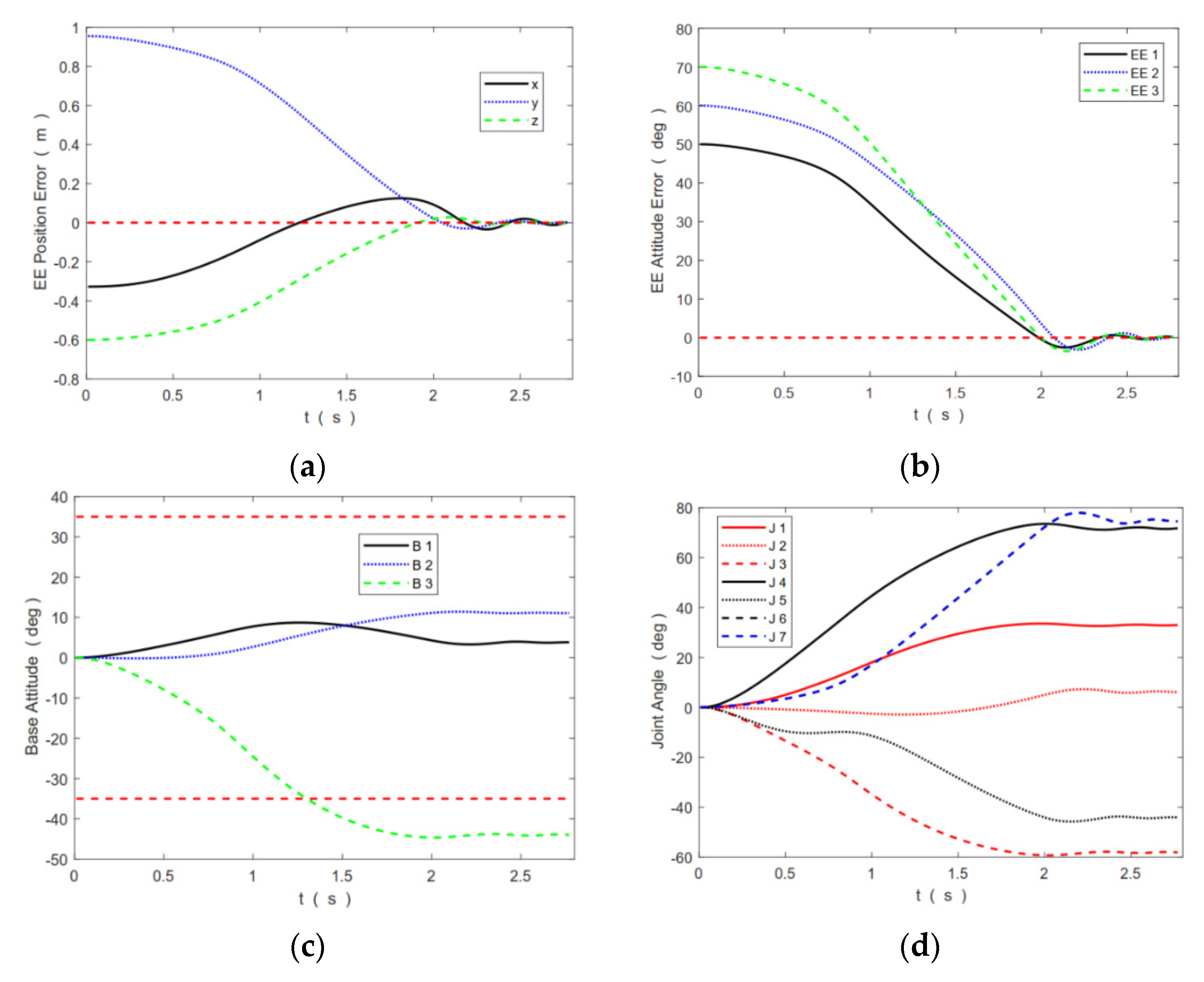
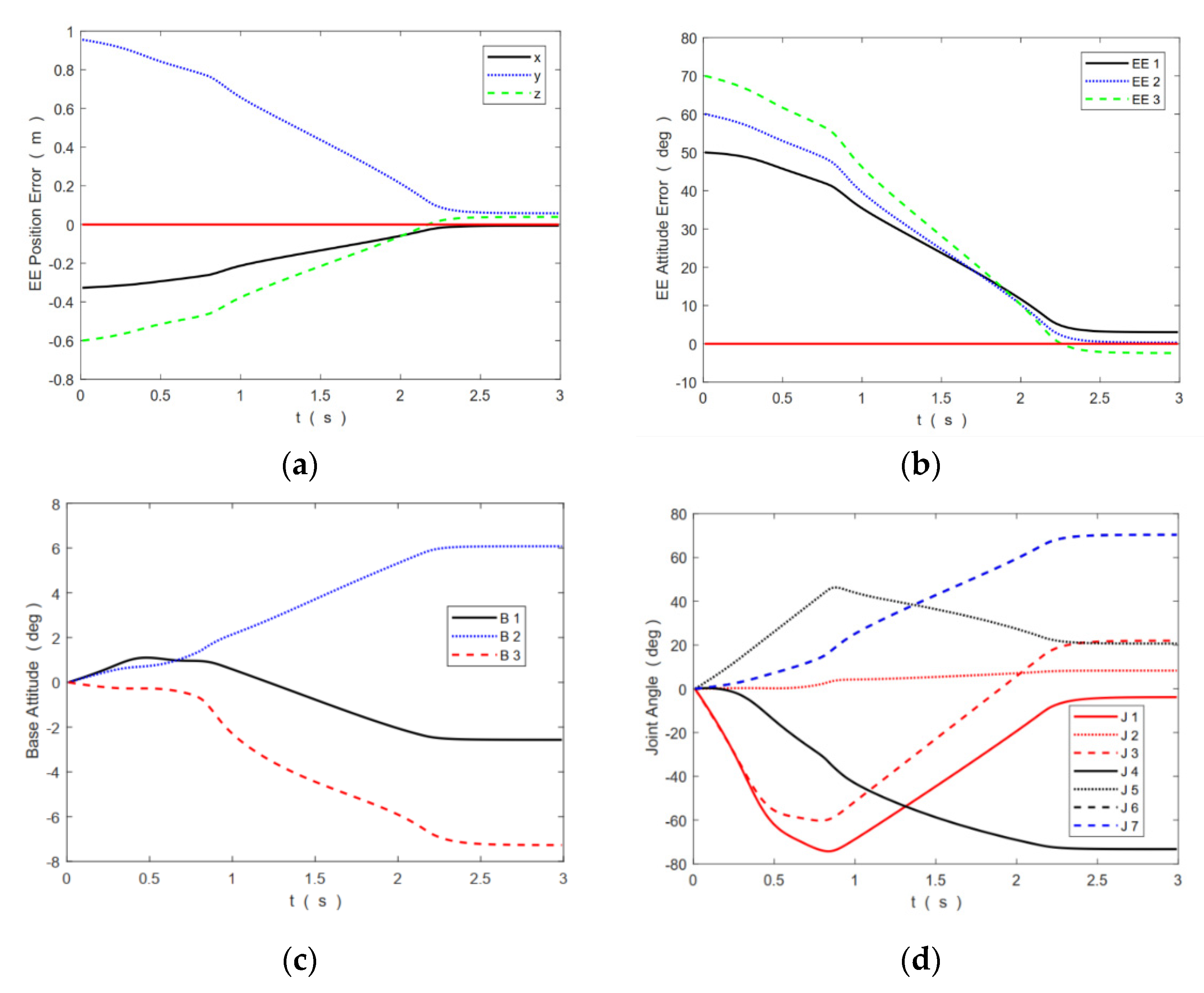
4.1. The Advantages of a Local Planner for Goal EE Pose Guiding Growth

This paper proposed a local planner that can adjust the attitude of the base when necessary. We compare it with the local planner based on the general Jacobian matrix and the local planner based on the extended Jacobian matrix by simulation. The former does not adjust the base attitude in the whole local planning process, and the latter always adjusts the base attitude in the whole local planning process. The local planner based on the general Jacobian matrix chooses actions according to the EE pose error in each iteration:

$$\dot{\mathit{\Theta }}={\left({\mathit{J}}_g\right)}^{+}\mathsf{\Delta }{\mathit{x}}_e$$

(25)

The local planner based on the extended Jacobian matrix chooses actions according to the EE pose error and the base attitude error in each iteration:

$$\dot{\mathit{\Theta }}={\left(\left[\begin{array}{c}{\mathit{H}}_{\omega }\\ {\mathit{J}}_g\end{array}\right]\right)}^{+}\left[\begin{array}{c}\Delta {\mathit{\Psi }}_b\\ \mathsf{\Delta }{\mathit{x}}_e\end{array}\right]$$

(26)

For these three local planners, the configuration parameters at the initial time are all set to $0^{°}$. The centroid position of the system is set to ${\left[\begin{array}{ccc}0& 0& 0\end{array}\right]}^{T}m$. The base attitude disturbance range is set as $\pm {35}^{\circ }$. The joint angle limit is set as $\pm {300}^{\circ }$. The reference goal base attitude is set as ${\left[\begin{array}{ccc}0& 0& 0\end{array}\right]}^{\circ }$ for the local planner for goal EE pose guiding growth proposed in this paper. For these three local planners, the goal EE position is ${\left[\begin{array}{ccc}6.8& 1& 2\end{array}\right]}^{T}m$ and the goal EE attitude is ${\left[\begin{array}{ccc}50& 60& 70\end{array}\right]}^{\circ }$.

Simulation results are shown in Figure 1, Figure 2 and Figure 3. From these results, we can see that the local planner based on the general Jacobian matrix can well achieve the EE pose goal, but the attitude of the base cannot meet the limit for this local planner. The local planner based on the extended Jacobian matrix can adjust the base attitude to a very low value. As the extended Jacobian matrix has more rows than columns, the local planner based on the extended Jacobian matrix cannot eliminate the EE pose error. Actually, for an FFSR, we only need to ensure that the base attitude disturbance meets the requirements. The main task for the motion planning of FFSRs is to drive its EE to a goal pose; there is no need to adjust its base attitude all the time. The local planner for the goal EE pose guiding growth proposed in this paper can not only ensure that the base attitude disturbance meets the requirements but also drive EE to a goal pose.

4.2. Verification of the Effectiveness of the Proposed RRTs for Free-Floating Space Robots

The simulation for the second part is divided into two scenarios: (1) Starting from the initial configuration and finally reaching the target EE position; (2) starting from the initial configuration and reaching the target EE pose. For these two scenarios, the configuration parameters at the initial time are all set to $0^{°}$. The centroid position of the system is set to ${\left[\begin{array}{ccc}0& 0& 0\end{array}\right]}^{T}m$. The base attitude disturbance range is set as $\pm {35}^{\circ }$. The joint angle limit is set as $\pm {300}^{\circ }$. The reference goal base attitude is set as ${\left[\begin{array}{ccc}0& 0& 0\end{array}\right]}^{\circ }$. For Scenario 1, the goal EE position is ${\left[\begin{array}{ccc}4& 2& 1\end{array}\right]}^{T}m$. For Scenario 2, the goal EE position is ${\left[\begin{array}{ccc}4& 3& 1\end{array}\right]}^{T}m$, and the goal EE attitude is ${\left[\begin{array}{ccc}50& 60& 70\end{array}\right]}^{\circ }$.

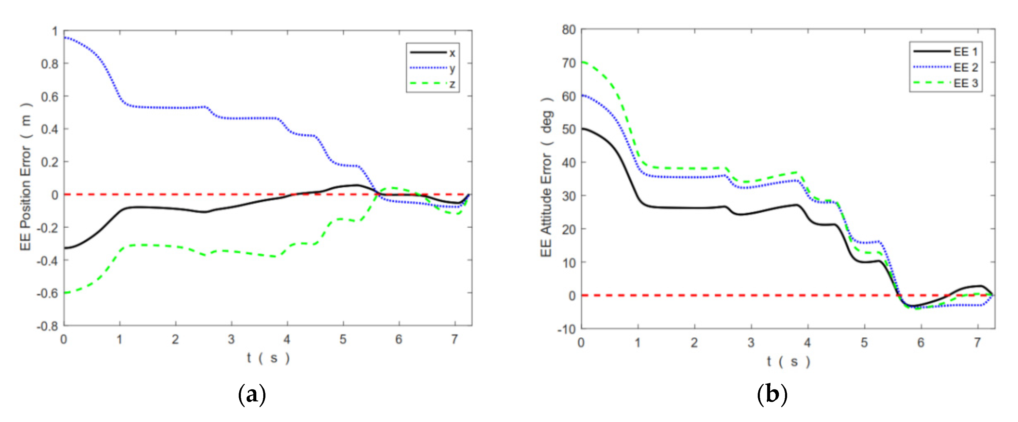
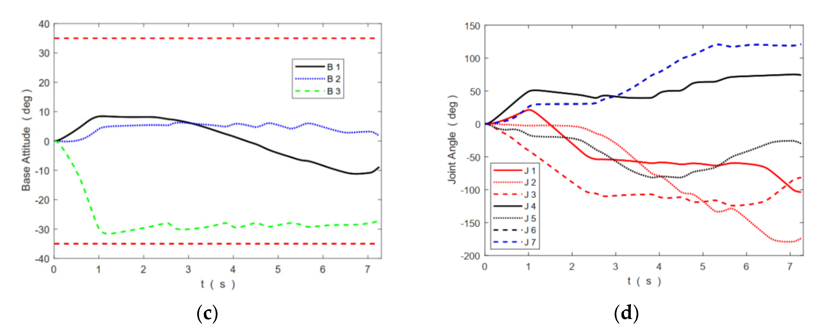
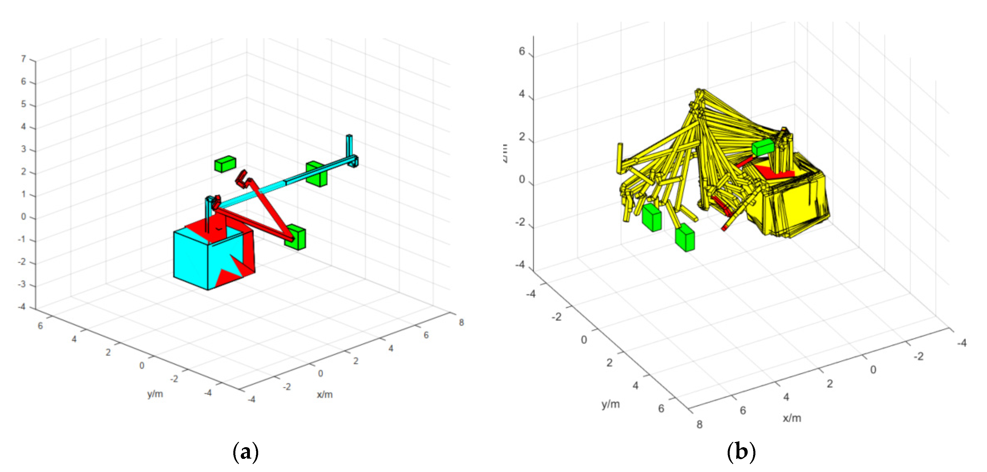
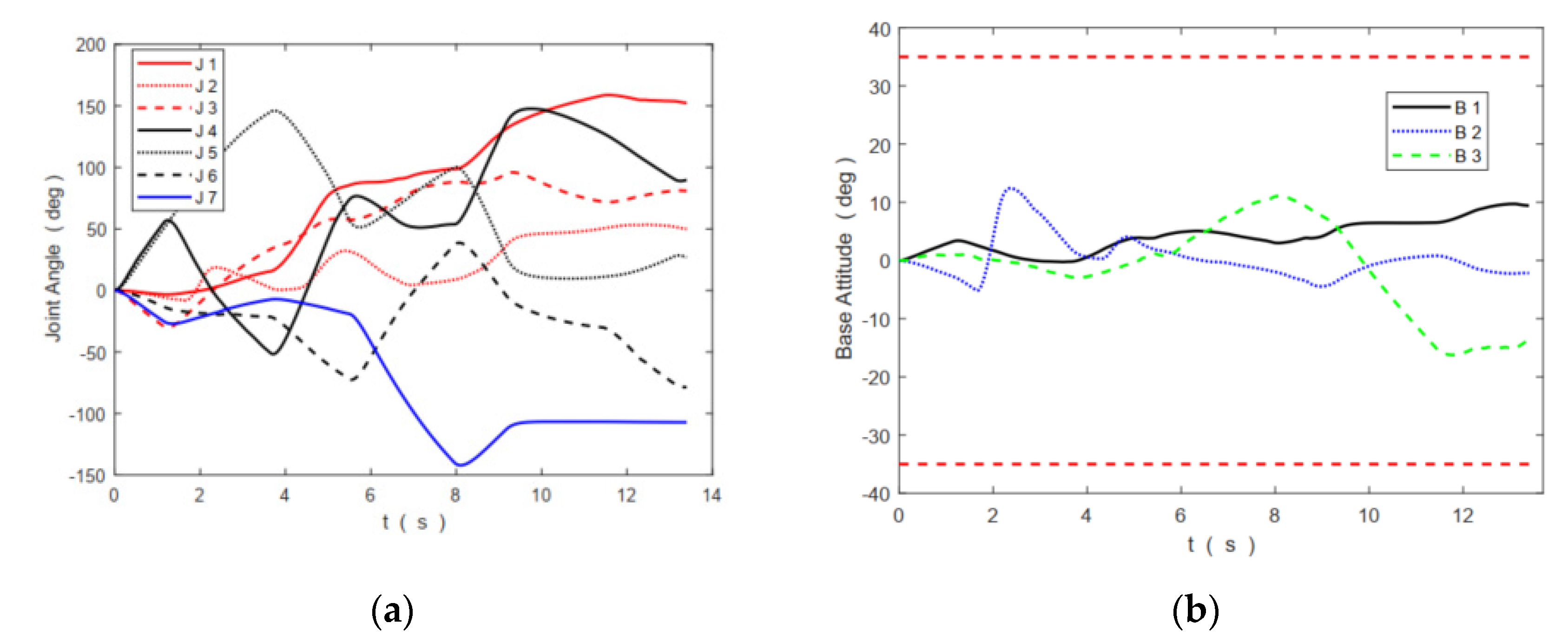
4.2.1. Simulation Results of Scenario 1

After 36 iterations, the FFSR reaches the target EE position. A generated configuration meets the requirements, as shown in Figure 4a. Figure 4b shows the movement history of the space robot from the initial configuration to the goal EE position and that the space robot does not collide with obstacles. Moreover, the rigid bodies of the space robot do not collide with each other. The joint trajectory and the base attitude disturbance trajectory are shown in Figure 5. It can be seen from Figure 5 that during the movement, the base attitude disturbance is effectively adjusted before reaching its limit.

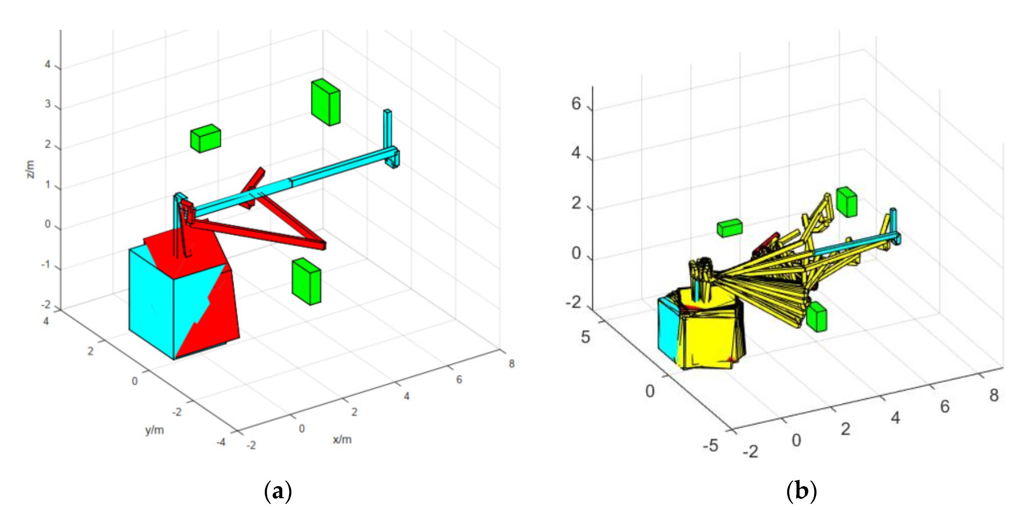
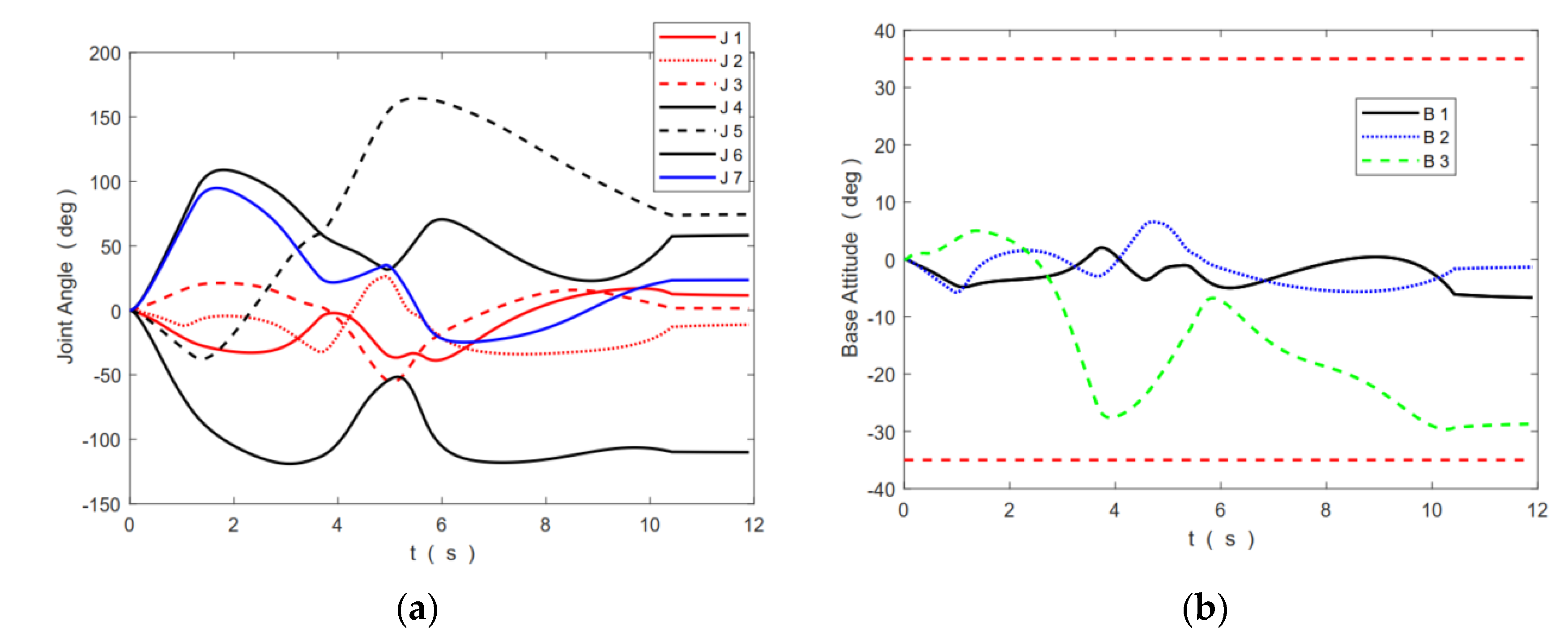
4.2.2. Simulation Results of Scenario 2

After 76 iterations, FFSR reaches the target EE pose. The generated configuration meets the requirements, as shown in Figure 6a. Figure 6b shows the movement history of the space robot from the initial configuration to the goal EE pose and that the space robot does not collide with obstacles. Moreover, the rigid bodies of the space robot do not collide with each other. The joint trajectory and the base attitude disturbance trajectory are shown in Figure 7. It can be seen from Figure 7 that during the movement, the base attitude disturbance is effectively adjusted before reaching its limit.

5. Conclusions

Based on the RRT framework, this paper designs a motion planner for FFSRs from an initial configuration to a goal EE pose. Compared with the existing works, it does not require us to solve the inverse kinematics. The differential constraints of FFSR can be handled by the designed local planners. Moreover, the planned trajectory meets the requirement that the attitude disturbance of its base does not exceed its limit. The main contribution is that two local planners are proposed to handle the special needs of motion planning of FFSRs:

• A control-based local planner for random configuration guiding growth of the tree. This planner uses the configuration error as a reference to select actions. It can achieve rapid local planning while taking into account the disturbance of the base.
• A control-based local planner for goal EE pose guiding growth of the tree. This local planner can adjust the attitude of the base when necessary. This planner mainly uses the EE pose error as a reference to select actions. Moreover, a reference goal base attitude and an error threshold for the base are introduced as a trigger for base attitude adjustment. The local planner based on this mechanism can make the base attitude disturbance meet the limit while avoiding singularity as much as possible.
• Finally, for collision detection, this paper proposes a method for calculating the position of the mass center of each rigid body of FFSRs in a certain configuration.

Sampling-based motion planning is an efficient way to deal with motion planning problems. This article systematically shows how to apply this kind of method to deal with the motion planning problem of FFSRs. Based on the framework proposed in this article, planners that can handle special planning problems of FFSRs can be easily designed.

References

1. Flores-Abad, A.; Ma, O.; Pham, K.; Ulrich, S. A review of space robotics technologies for on-orbit servicing. Prog. Aerosp. Sci. 2014, 68, 1–26. [Google Scholar] [CrossRef] [Green Version]
2. Elbanhawi, M.; Simic, M. Sampling-based robot motion planning: A review. IEEE. Access. 2014, 2, 56–77. [Google Scholar] [CrossRef]
3. Lynch, K.M.; Park, F.C. Modern Robotics; Cambridge University Press: Cambridge, UK, 2017; pp. 325–348. [Google Scholar]
4. Vafa, Z.; Dubowsky, S. On the dynamics of manipulators in space using the virtual manipulator approach. In Proceedings of the IEEE International Conference on Robotics and Automation, Raleigh, NC, USA, 31 March–3 April 1987; pp. 579–585. [Google Scholar]
5. Vafa, Z.; Dubowsky, S. On the dynamics of space manipulators using the virtual manipulator, with applications to path planning. In Space Robotics: Dynamics and Control; Xu, Y., Kanade, T., Eds.; Springer: Boston, MA, USA, 1993; pp. 45–76. [Google Scholar]
6. Nakamura, Y.; Mukherjee, R. Non-holonomic path planning of space robots via bi-directional approach. In Proceedings of the IEEE International Conference on Robotics and Automation, Cincinnati, OH, USA, 13–18 May 1990; pp. 1764–1769. [Google Scholar]
7. Fernandes, C.; Gurvits, L.; Li, Z. Near-optimal non-holonomic motion planning for a system of coupled rigid bodies. IEEE Trans. Automat. Contr. 1994, 39, 450–463. [Google Scholar] [CrossRef]
8. Yamada, K. Arm path planning for a space robot. In Proceedings of the IEEE/RSJ International Conference on Intelligent Robots and Systems, Yokohama, Japan, 26–30 July 1993; pp. 2049–2055. [Google Scholar] [CrossRef]
9. Suzuki, T.; Nakamura, Y. Planning spiral motion of non-holonomic space robots. In Proceedings of the IEEE International Conference on Robotics and Automation, Minneapolis, MN, USA, 22–28 April 1996; pp. 718–725. [Google Scholar]
10. Lampariello, R. Motion Planning for the On-orbit Grasping of a Non-cooperative Target Satellite with Collision Avoidance. In Proceedings of the 10th International symposium on Artificial Intelligence, Robotics and Automation in Space, Sapporo, Japan, 29 August–1 September 2010. [Google Scholar]
11. Schulman, J.; Duan, Y.; Ho, J.; Lee, A.; Awwal, I.; Bradlow, H.; Pan, J.; Patil, S.; Goldberg, K.; Abbeel, P. Motion planning with sequential convex optimization and convex collision checking. Int. J. Robot. Res. 2014, 33, 1251–1270. [Google Scholar] [CrossRef] [Green Version]
12. Zucker, M.; Ratliff, N.; Dragan, A.D.; Pivtoraiko, M.; Klingensmith, M.; Dellin, C.M.; Bagnell, J.A.; Srinivasa, S.S. Chomp: Covariant hamiltonian optimization for motion planning. Int. J. Robot. Res. 2013, 32, 1164–1193. [Google Scholar] [CrossRef] [Green Version]
13. Kalakrishnan, M.; Chitta, S.; Theodorou, E.; Pastor, P.; Schaal, S. STOMP: Stochastic trajectory optimization for motion planning. In Proceedings of the IEEE International Conference on Robotics and Automation, Shanghai, China, 9–13 May 2011; pp. 4569–4574. [Google Scholar]
14. Misra, G.; Bai, X. Task-constrained trajectory planning of free-floating space-robotic systems using convex optimization. J. Guid. Control. Dyn. 2017, 40, 2857–2870. [Google Scholar] [CrossRef]
15. Virgili-Llop, J.; Zagaris, C.; Zappulla, R.; Bradstreet, A.; Romano, M. A convex-programming-based guidance algorithm to capture a tumbling object on orbit using a spacecraft equipped with a robotic manipulator. Int. J. Robot. Res. 2019, 38, 40–72. [Google Scholar] [CrossRef]
16. Wang, M.; Luo, J.; Walter, U. Trajectory planning of FFSRusing Particle Swarm Optimization (PSO). Acta Astronaut. 2015, 112, 77–88. [Google Scholar] [CrossRef]
17. Xu, W.; Li, C.; Wang, X.; Liu, Y.; Liang, B.; Xu, Y. Study on non-holonomic cartesian path planning of a free-floating space robotic system. Adv. Robot. 2009, 23, 113–143. [Google Scholar] [CrossRef]
18. Wang, M.; Luo, J.; Fang, J.; Yuan, J. Optimal trajectory planning of free-floating space manipulator using differential evolution algorithm. Adv. Space Res. 2018, 61, 1525–1536. [Google Scholar] [CrossRef]
19. Bertram, D.; Kuffner, J.; Dillmann, R.; Asfour, T. An integrated approach to inverse kinematics and path planning for redundant manipulators. In Proceedings of the IEEE International Conference on Robotics and Automation, Orlando, FL, USA, 15–19 May 2006; pp. 1874–1879. [Google Scholar]
20. Weghe, M.V.; Ferguson, D.; Srinivasa, S.S. Randomized path planning for redundant manipulators without inverse kinematics. In Proceedings of the IEEE-RAS International Conference on Humanoid Robots, Pittsburgh, PA, USA, 29 November–1 December 2007; pp. 477–482. [Google Scholar]
Figure 1. Time histories of EE position error, EE attitude error, base attitude trajectory, and joint trajectory for the local planner based on the general Jacobian matrix. (a) Time histories of EE position error; (b) time histories of EE attitude error; (c) time histories of base attitude trajectory; (d) time histories of joint trajectory.
Applsci 10 09137 g001
Figure 2. Time histories of EE position error, EE attitude error, base attitude trajectory, and joint trajectory for local planner based on the extended Jacobian matrix. (a) Time histories of EE position error; (b) time histories of EE attitude error; (c) time histories of base attitude trajectory; (d) time histories of joint trajectory.
Applsci 10 09137 g002
Figure 3. Time histories of EE position error, EE attitude error, base attitude trajectory, and joint trajectory of local planner for goal EE pose guiding growth. (a) Time histories of EE position error; (b) time histories of EE attitude error; (c) time histories of base attitude trajectory; (d) time histories of joint angle.
Applsci 10 09137 g003aApplsci 10 09137 g003b
Figure 4. Initial configuration, final configuration, and movement history of the space robot in Scenario 1. (a) The final configuration solved by the planning algorithm in Scenario 1; (b) The movement history of the space robot from the initial configuration to the goal EE position in Scenario 1.
Applsci 10 09137 g004
Figure 5. Joint trajectory and base attitude disturbance trajectory for Scenario 1. (a) Joint trajectory; (b) base attitude disturbance trajectory.
Applsci 10 09137 g005
Figure 6. Initial configuration, final configuration, and movement history of the space robot in Scenario 2. (a) The initial configuration and the final configuration solved by the planning algorithm in Scenario 2; (b) the movement history of the space robot from the initial configuration to the goal EE pose in Scenario 2.
Applsci 10 09137 g006
Figure 7. Joint trajectory and base attitude disturbance trajectory for Scenario 2. (a) Joint trajectory; (b) base attitude disturbance trajectory.
Applsci 10 09137 g007