Autonomous Underwater Vehicle Localization Using Sound Measurements of Passing Ships


Electronic and Electrical Convergence Department, Hongik University, Sejong 2639, Korea
Appl. Sci. 2020, 10(24), 9139; https://doi.org/10.3390/app10249139
Submission received: 30 November 2020
/
Revised: 16 December 2020
/
Accepted: 17 December 2020
/
Published: 21 December 2020
(This article belongs to the Special Issue Advances in Robot Path Planning)
Abstract
:This paper introduces the localization method of an Autonomous Underwater Vehicle (AUV) in environments (such as harbors or ports) where there can be passing ships near the AUV. It is assumed that the AUV can access the trajectory and approximate source level of a passing ship, while identifying the ship by processing the ship’s sound. This paper considers an AUV which can localize itself by integrating propeller and Inertial Measurement Units (IMU). Suppose that the AUV has been moving in underwater environments for a long time, under the IMU-only localization. To fix long-term drift in the IMU-only localization, we propose that the AUV localization uses sound measurements of passing ships whose trajectories are known a priori. As far as we know, this AUV localization method is novel in using sound measurements of passing ships of which the trajectories are known a priori. The performance of the proposed localization method is verified utilizing MATLAB simulations. The simulation results show significant estimation improvements, compared to IMU-only localization. Moreover, using measurements from multiple ships gives better estimation results, compared to the case where the measurement of a single ship is used.
1. Introduction
The localization problem of an Autonomous Underwater Vehicle (AUV) is a critical problem for the navigation of the AUV. This paper presents the localization of an AUV in environments (such as harbors or ports) where there can be passing ships near the AUV. In practice, there may be ships with known trajectories. We assume that the AUV can access the trajectory and approximate Source Level (SL) of a passing ship, while identifying the ship by processing the sound of the ship. The proposed localization method uses sound bearing measurements of a passing ship moving along a known trajectory (planned routes).
We use the planned routes of large commercial ships. Large commercial ships make large noise, thus their sound signals travel a long distance in underwater environments. Hence, the sound information of large commercial ships is valuable for the proposed localization. The information of ships’ trajectories is accessible, since a ship uses Automatic Identification System (AIS) nowadays. AIS records the position, routes, destinations of large commercial ships worldwide. The AIS of commercial ships is available using the following website: https://www.marinetraffic.com/.
It is feasible that the AUV can access approximate Source Level (SL) of a passing ship, while identifying the ship by processing the sound of the ship. McKenna et al. [1] introduced metrics of ship noise, including spatial radiation patterns, source levels, spectral characteristics, and sound exposure levels for seven merchant ship-types: container ships, vehicle carriers, bulk carriers, open-hatch cargo ships, and chemical, crude oil and product tankers. It is feasible to gather the SL information of large commercial ships using the estimation approach in [2]. Jiang et al. [3] acquired the noise data from a large number of individual ships, and calculated sound transmission loss (TL) to estimate ship source levels. Then, the relationship between ship noise source level and different parameters was analyzed; the mean source spectrum curve of selected ships was fitted; and the source spectrum model for merchant ship-radiated noise was established. The authors of [4] provided frequency analysis methods for estimating ship machinery sources and propeller noise.
In the past, various localization techniques (acoustic, geophysical, optical, or sensor fusion methods) were used for underwater localization [5]. To localize an AUV by processing signal measurements, Time-Of-Arrival (TOA) [6,7,8,9], Time-Difference-Of-Arrival (TDOA) [10,11,12], or Angle-Of-Arrival (AOA) [13,14] can be used. In practice, short-BaseLine (SBL) [15], Ultra-Short-BaseLine (USBL) [16], and Long-BaseLine (LBL) [17] were widely used to track underwater vehicles and divers. However, SBL, USBL, or LBL require additional facilities, such as signal transmitters and receivers.
Many papers [18,19,20,21] discussed Cooperative Localization (CL) of an AUV assisted by a surface vehicle, say Communication Navigation Aid (CNA), which can utilize Global Positioning Systems (GPS) to localize itself. Bahr er al. and Cao et al. [18,22] handled the case where the AUV’s motion is constrained by the CNA’s motion. The CNA locates an AUV by measuring the relative position (or distance) of the AUV in [18,19]. Several papers discussed cooperative localization of AUVs based on bearing-only [23,24] or range-only measurements [25]. However, this paper handles the case where only one AUV exists, thus no CNA can be used for the AUV’s localization.
Consider the case where only one AUV exists, as in this paper. Allotta et al. [26,27] integrated propeller and Inertial Measurement Units (IMU) for localization of the AUV. In the case where the AUV moves close to the sea bottom, Doppler Velocity Log (DVL) can be integrated to measure the AUV speed with respect to the ground [26,27,28]. In [29], sensor fusion models that incorporate gyroscope, accelerometer and ultrasound sensors were presented. The robot pose can be estimated using the Extended Kalman Filter (EKF) to remove biases from IMU. In underwater environments, Melim et al. [30] considered visual Simultaneous Localization and Mapping (SLAM) using a high frequency imaging sonar. Corke et al. [31] described an experiment in which two methods (visual odometry and using a field of static nodes) of underwater robot localization were compared.
Visual odometry or Visual SLAM are based on integrating perceived motion of the AUV. These methods are subject to long-term drift, and require occasional position fixes in order to maintain a low localization error. Moreover, Visual odometry or Visual SLAM require a high frequency imaging sonar, which consumes an AUV’s power resource significantly. Thus, it is desirable to use a passive navigation solution for an AUV. Using a field of static nodes involves the creation of infrastructure which must be powered, but provides absolute position estimates. This paper considers an AUV, which can locate itself by integrating propeller and IMU (IMU-only localization) [26,27]. Suppose that using the IMU-only localization, the AUV has been moving in underwater environments for a long time. This IMU-only localization is based on integrating perceived motion of the AUV. Thus, as the AUV stays longer in underwater environments, its localization error keeps growing.
Recall that this paper presents the localization of an AUV in environments (such as harbors or ports) where there can be passing ships near the AUV. Thus, operation in the open sea is not within the scope of this paper. To fix long-term drift in the IMU-only localization, this paper proposes that the AUV localization utilizes the sound measurements of passing ships of which the trajectories are known a priori. These ships can be considered as “a field of moving nodes” to fix localization of the AUV.
This paper handles the case where the target (passing ship in this paper) information is known, and the observer (AUV in this paper) trajectory is to be estimated using bearing measurements associated to the passing ships. Tracking a target using bearing-only measurements is termed the Bearing-Only Target Motion Analysis (BOTMA) problem [32,33,34,35]. The observer maneuver is needed to observe the target state (position and velocity) in the BOTMA problem [36].
The proposed localization scheme can be considered as the reverse process of the BOTMA. In the considered localization problem, the AUV’s velocity can be conjectured by integrating propeller and IMU [26,27]. The error in this integration is modeled using a process noise.
To solve the BOTMA problem, Range Parameterized EKF (RPEKF) was used to reduce the range estimation error [37,38]. The EKF is suitable for real-time processing of nonlinear systems, since it is computationally efficient [34]. The RPEKF is composed of many independent EKFs, such that every EKF has a different initial range estimation. The combined target estimation is derived as a weighted sum of every EKF output.
If the AUV cannot measure the sound of any ship, then it relies on locating itself by integrating propeller and IMU (IMU-only localization). We assume that the AUV has been moving in underwater environments using the IMU-only localization before time step 0. Note that the range between a ship and the AUV is not accessible at time step 0, due to long-term drift of the AUV. Thus, this paper modifies the RPEKF to decrease the range estimation error.
Moreover, there may be a case where the long-term drift of the AUV is too severe. Assume that the AUV can access the approximate SL of a passing ship. Based on the SL, we can utilize an acoustic propagation model, which simulates the sound emanated from the ship. Environmental factors, such as underwater obstacles or topographical maps, can be taken into account in the modeling of an acoustic propagation model. The Range-dependent Acoustic Model (RAM) [39,40,41] has been widely used to simulate how the sound signal of the ship propagates in underwater environments. Using RAM, we can derive the feasible region where the AUV can exist, in order to measure the sound of the ship. Then, the RPEKF is applied to estimate the AUV position, considering the feasible region.
The contributions of this paper are summarized as follows. This paper assumes that the AUV can access the trajectory and source level of a passing ship, while identifying the ship by processing the ship’s sound. To fix long-term drift in the IMU-only localization, we introduce the AUV localization method using sound measurements of passing ships that travel along known routes. Under the proposed localization method based on moving ships, we do not have to create additional infrastructure for AUV localization. Moreover, we can localize the AUV in a stealthy and power-efficient manner, since the AUV does not emit a signal during this passive localization. As far as we know, this AUV localization method is novel in using sound measurements of passing ships of which the trajectories are known a priori. This paper is novel in presenting the underwater localization method using RAM and sound measurements of ships moving along known routes. We verify the effectiveness of the proposed localization method utilizing MATLAB simulations.
This paper is organized as follows. Section 2 presents the preliminary information of the paper. Section 3 presents the localization method using bearing-only measurements of passing ships. Section 4 presents MATLAB simulations to verify the effectiveness of the proposed localization method. Section 5 provides Conclusions.
2. Preliminary Information
2.1. Extended Kalman Filter (EKF)
The range between a ship and the AUV is not accessible at time step 0, due to long-term drift of the AUV. Thus, this paper uses the RPEKF to decrease the range estimation error. The RPEKF is composed of many independent EKFs, such that every EKF has a different initial range estimation.
As the preliminary information of this paper, we introduce the EKF in [34] briefly. We consider discrete-time systems. indicates the sampling duration of our discrete-time system. At sample-index k, we can define a nonlinear process model as
Here, denotes the state vector at sample-index k. Also, is a Gaussian noise with mean and covariance matrix .
At sample-index k, we can define a nonlinear measurement model as
Here, is a Gaussian noise with mean and covariance matrix .
Let denote the state vector of the EKF, utilizing all measurements up to sample-index k. In addition, denotes the error covariance of . The EKF is composed of the prediction step and the measurement update.
Using Equation (1), we predict the state vector of the EKF as
We then predict the error covariance matrix as
Here, is the partial derivative of with respect to evaluated at .
Using the measurement in Equation (2), the state vector of the EKF is updated as
Here, we use
where is the partial derivative of with respect to evaluated at . The error covariance is updated using
Then, we update both the state vector and its error covariance using
2.2. Derive the Maximum Sensing Range Associated to a Ship
As the preliminary information of this paper, we introduce the propagation model which simulates a sound field in underwater environments [41]. While the surface target’s sound signal propagates in underwater environments, a sound field generated from the target gets complicated due to environmental interference [42]. Numerical propagation models, such as ray theory and parabolic equation, were widely utilized to simulate a sound field [41].
In the parabolic equation, a small-angle approximation approximates the elliptic wave equation obtained from the Helmholtz equation. However, this results in error at steep angle spaces. RAM reduces this error utilizing a wide-angle parabolic equation with Pade approximation [39,40,41]. In this way, RAM can simulate a sound field accurately.
Next, several definitions in [42] are discussed. Source Level () indicates the sound strength generated by a source. We assume that the approximate of a ship is known a priori. Transmission Loss () is the reduction of sound while the sound emanates from the source. profile is the function of both target range and depth.
represents of the target’s signal as the AUV is at a position C and the source is at a position . is constructed utilizing the RAM. Let denote the sound strength as the sound signal from the target at reaches the AUV in C. is estimated as
Note that the AUV at C fails to measure the sound of the target ship at in the case where is less than zero. Using Equation (9), the AUV cannot measure the ship’s sound in the case where
is met. The AUV’s depth can be measured using pressure sensors. Thus, the maximum sensing range can be derived by searching for a target range, which satisfies Equation (10).
2.3. RPEKF
The RPEKF in [37,38] is utilized to decrease the range estimation error. In the RPEKF, we utilize M EKF tracks to decrease the range estimation error. Every EKF track of the RPEKF runs the EKF in Section 3.2 independently, such that every EKF has a different initial range estimate.
We assume that the AUV has been moving in underwater environments using the IMU-only localization before time step 0. Suppose that at time step 0, the IMU-only localization estimates the range between the ship and the AUV as . Also, suppose that the range estimation error at time step 0 is bounded above by . Doing underwater experiments, we can derive the relationship between the operation time of the AUV (under the IMU-only localization) and the increase in localization error. Then, the bound for localization error can be set considering the operation time of the AUV in underwater environments. This range estimation error is unavoidable, since the AUV has been moving in underwater environments using the IMU-only localization.
A feasible range interval () is set considering the localization error of the AUV at time step 0. Here, is set as
Also, we use
Moreover, there may be a case where the long-term drift of the AUV is too severe. Assume that the AUV can access the approximate SL of a passing ship. Based on the SL, we can utilize an acoustic propagation model, which simulates the sound emanated from the ship. Suppose that the AUV measures the sound of the ship. Then, using the RAM in Section 2.2, we can derive the feasible region where the AUV can exist.
For instance, suppose that the maximum sensing range, say , is derived by searching for a target range satisfying Equation (10). In this case, we use
instead of Equation (11). Also, we use
instead of Equation (12).
To maintain a comparable performance of every EKF track, the range interval () is divided such that the j-th sub-interval has its range interval as () for .
We utilize . For , we utilize
Here,
Thus, we have .
In total, M EKF tracks are utilized, and we utilize the likelihood () from the j-th EKF track. In , is in Equation (2).
Let denote the state vector of the j-th EKF track, utilizing all measurements up to sample-index k. In addition, denotes the error covariance of . Let denote the state vector of the j-th EKF track, utilizing all measurements up to sample-index .
Let for convenience. The weight of the j-th EKF track () is
In Equation (17), the likelihood is derived as
Here, , , and .
The state vector and its error covariance at sample-index k are calculated as
At sample-index 0, we set where . At each sample-index k, is updated utilizing
3. The Localization Method Using Bearing-Only Measurements
3.1. System Models
This manuscript considers horizontal AUV motion in two dimensions. In other words, the AUV maneuvers while maintaining a certain depth. The AUV’s depth can be measured fairly well by utilizing pressure sensors.
We first introduce some notations used in this paper. presents the identity matrix with r rows and r columns. Let indicate a diagonal matrix with diagonal elements in this order. is used to present the error covariance of a variable . Let denote the argument (also called phase or angle) of the complex number, say .
Suppose that the AUV measures the sound of N ships in total. () is the vector representing the position of the n-th ship at sample-index k. is the 2D vector representing the velocity of the n-th ship at sample-index k.
We assume that the AUV can access the trajectory of a passing ship, while identifying the ship by processing the sound of the ship. This implies that the AUV at sample-index k can access for all .
Let denote the 2D vector representing the position of the AUV at sample-index k. Let denote the 2D vector representing the velocity of the AUV at sample-index k. Let
denote the state vector representing the AUV state.
Recall that denotes the sampling interval in the discrete-time systems. The discrete-time process model of the AUV is
The AUV velocity can be estimated by integrating propeller and IMU. We can estimate the AUV velocity using the integration approach in [26,27]. Considering the process noise in the estimation, Equation (23) can be rewritten as
In (24), is
Also, is
In (24),
presents the process noise. Here, presents the AUV’s 2D acceleration noise, which is unknown a priori. In , we utilize
The process noise is added in (24), considering the error in estimating as we integrate propeller and IMU. In (24), is assumed to be derived by integrating propeller and IMU [26,27]. For instance, unknown sea currents can generate large process noise [26]. In (24), is a Gaussian noise with mean and covariance matrix .
The proposed localization scheme can be considered as the reverse process of the BOTMA. The proposed localization method uses sound bearing measurements of a passing ship moving along a known trajectory (planned routes). Let denote the bearing measurement associated to the n-th ship () at sample-index k. The bearing measurement model associated to the n-th ship () is
Here, we utilize
Here, , and . In (29), is the measurement noise with following distribution: . Here, represents Gaussian distribution with mean and covariance matrix .
Recall that is the partial derivative of with respect to evaluated at . See Equation (6). We next present how to derive . We utilize
Here, . Furthermore, we utilize
Using Equation (30), we have
3.2. Run the RPEKF Based on Bearing-Only Measurements of Passing Ships
This subsection presents running the RPEKF based on bearing-only measurements of passing ships. We discuss how to update the EKF track in the RPEKF (See Section 2.3).
Recall that the superscript in Section 2.3 denotes the index of each EKF track in the RPEKF (See Section 2.3). The EKF is composed of two steps: prediction step and measurement update step.
3.2.1. Prediction Step
We first present the prediction step. As the process model (1), we utilize the linear model in (24). Since our model is linear, the prediction step is
Based on Equation (4), we further predict the error covariance matrix using
3.2.2. Measurement Update Step
We next present the measurement update step in the EKF. Suppose that the AUV measures the bearing of sound of ships at sample-index k. Let denote the index of the measured ship at sample-index k. Since there are N ships in total, we have
Using Equation (29), the measurement associated to the -th ship () is
In each EKF track, we perform the EKF measurement update associated to each ship in . The EKF measurement update indicates that we apply the EKF Equations (6) and (7) sequentially.
We have measurements at sample-index k. Thus, each EKF track keeps running the Equations (6) and (7) times iteratively, while using measurements in Equation (38). In other words, each EKF track uses as the first measurement at sample-index k. The EKF track applies the Equations (6) and (7), while using as the measurement in Equation (5). Next, the track uses as the second measurement at sample-index k. The EKF track applies the Equations (6) and (7), while using as the measurement in Equation (5). Iterate this until the track uses as the last measurement at sample-index k. The EKF track applies the Equations (6) and (7), while using as the measurement in Equation (5).
In this way, each EKF track can process the sound of ships at sample-index k. Once the measurement update is done using measurements at sample-index k, each EKF track updates both the state vector and its error covariance using Equation (8).
3.2.3. Outlier Measurement Handing
In some cases, a bearing measurement may not be accurate enough to update the KF estimation. Considering this aspect, a bearing measurement is discarded in the case where a bearing measurement satisfies the following condition.
where , and . Recall the measurement Equation (2). In the case where the measurement has a Gaussian distribution with mean 0 and covariance , is also Gaussian with mean 0 and covariance . (39) implies that this paper does not utilize a bearing measurement, which is npt reliable considering the KF estimation. If the condition in (39) is satisfied, then we do not perform the measurement update associated to the bearing measurement.
In (39), is a tuning parameter. We use in the simulations. We present why is set as 5. Suppose is an observation from a normally distributed random variable, is the mean of the distribution, and is its standard deviation. Then, we have
Here, is the probability that a sample in exists between and . Using the property in (40), we use .
4. MATLAB Simulations
We use MATLAB (MathWorks, Natick, MA, USA) simulations to demonstrate the performance of the proposed localization approach. The scenario runs for 3000 s. The sampling duration is second.
In Equation (29), the bearing measurement noise is set as degrees. This bearing noise model is commonly used in the literature on target tracking based on bearing measurements [32,33,34,35].
This paper considers the AUV that can locate itself by integrating a propeller and IMU. We set the noise in the simulations as follows. Let represent the standard deviation of a. In Equation (27), we utilize . This process noise is set considering the error in estimating , as the AUV integrates propeller and IMU for its localization [26,27].
Using the IMU-only localization, the AUV has been moving in underwater environments before time step 0. Suppose that at time step 0, the IMU-only localization estimates the range between the 1-st ship and the AUV as m. Also, suppose that the range estimation error at time step 0 is bounded above by m. Using Equations (11) and (12), we set m, and m. Also, EKF tracks are used in total.
The j-th EKF track () has its initial state vector as
Here, . Recall that is defined in Equation (15). In Equation (41), indicates a zero vector with two columns. Recall that in Equation (41) is the bearing measurement associated to the 1-st ship at sample-index 0.
Furthermore, we have
Considering the j-th EKF track, is selected as
Here, is the maximum speed of an AUV, which is assumed to be known a priori. We utilize m per second. In Equation (45), indicates a 2 by 2 zero matrix.
We run Monte-Carlo simulations. where is the AUV position estimation at sample-index k utilizing the m-th Monte-Carlo simulation. is the error of the AUV position estimation at sample-index k.
At the m-th Monte-Carlo simulation (), one considers the estimation error, given by
Then, at each sample-index k, the following metric is utilized:
Also, at each sample-index k, we define
and
In simulations, we plot , , and with respect to sample-index k.
4.1. One Ship Scenario
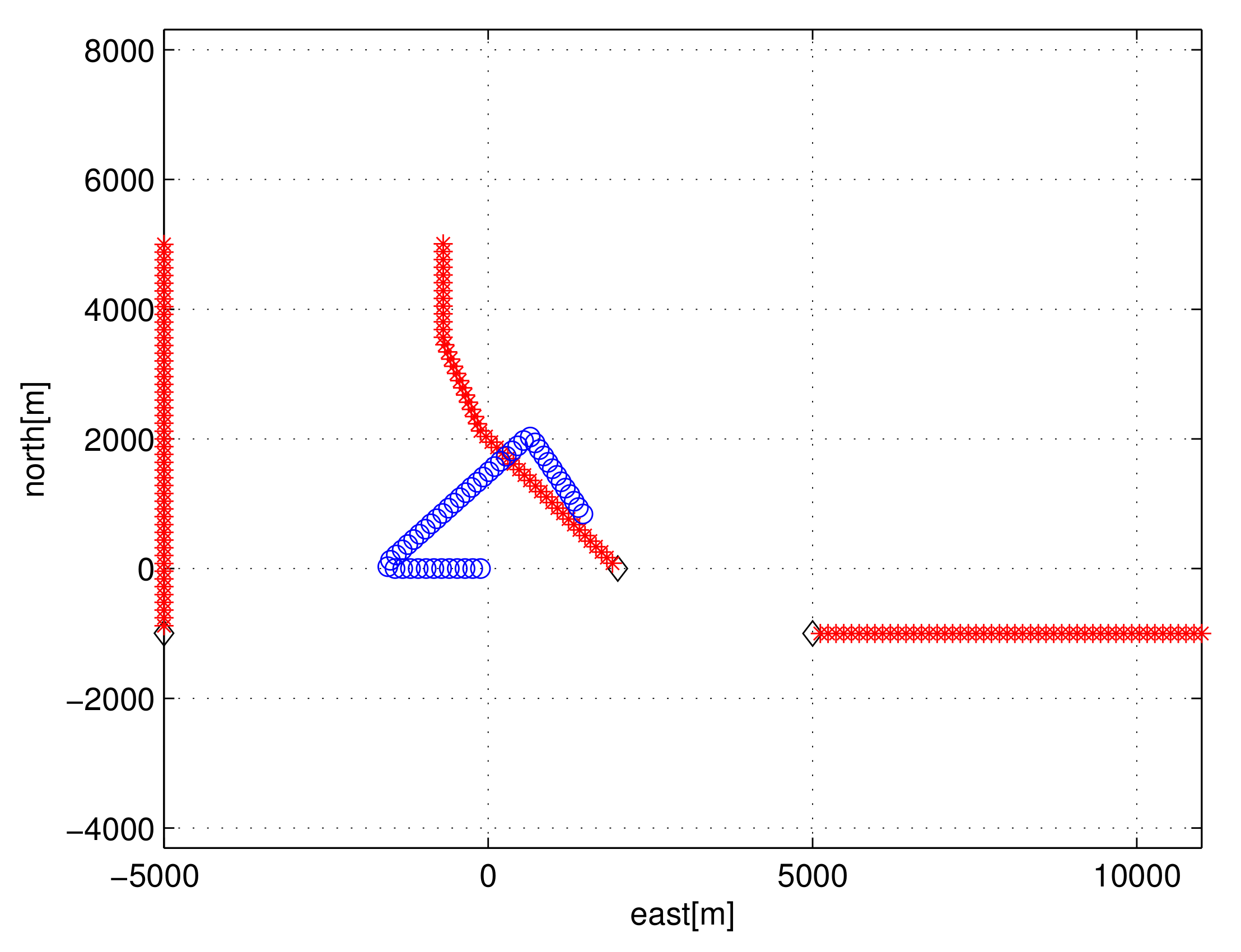
Figure 1 presents the scenario using one ship. The speed of the ship is 2 m/s, and that of the AUV is 2 m/s. The AUV starts from the origin. The ship starts from (2000,0) in meters, and the trajectory of the ship at every minute is plotted with red asterisks. The starting point of the ship is marked with a diamond. The trajectory of the AUV at every minute is depicted with blue circles.
Consider the case where the proposed localization method is utilized. In Figure 2, we plot , , and with respect to sample-index k. The AUV maneuvers at 750 and 2250 s. At these moments, the estimation error decreases sharply. This is similar to the case where the maneuver of an observer makes the BOTMA system observable [36].
To run one Monte-Carlo simulation takes about 1.3 s utilizing MATLAB simulations. See that the computational load of the proposed localization scheme is very low.
4.2. Three Ships Scenario
We next consider the scenario with three ships. The speed of every ship is 2 m/s, and that of the AUV is 2 m/s. The AUV starts from the origin. In Figure 3, the starting point of each ship is marked with a diamond. At every minute, the trajectory of every ship is plotted with red asterisks. At every minute, the trajectory of the AUV is depicted with blue circles.
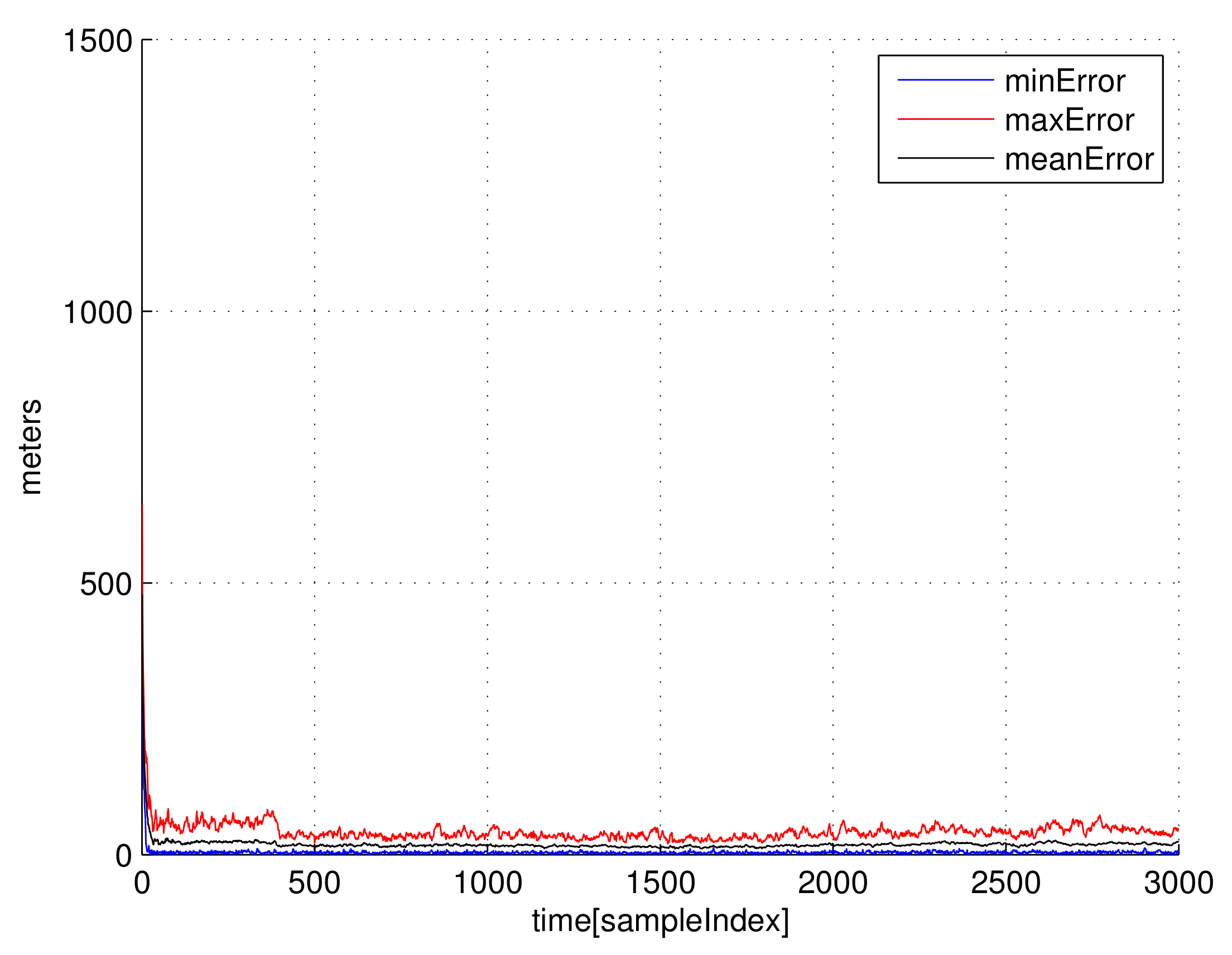
Consider the case where the proposed localization method is utilized, while using three ships. In Figure 4, we plot , , and with respect to sample-index k. See that the estimation error decreased considerably, compared to Figure 2. This is due to the fact that the AUV localization uses three bearing lines emitted from three ships, instead of one bearing line emitted from one ship. To run one Monte-Carlo simulation takes about 2.6 s utilizing MATLAB simulations. See that the computational load of the proposed localization scheme is very low.
4.3. IMU-Only Localization
For comparison, we consider the case where the AUV localizes itself by integrating propeller and IMU. Note that no ships are used in this IMU-only localization. The movement of the AUV is identical to that in Figure 1. Similarly to Equation (24), the AUV can locate itself using
Here, is in Equation (26), and is in Equation (27). in (50) is assumed to be derived by integrating a propeller and IMU [26,27]. The error in the IMU integration is modeled by adding Gaussian noise in Equation (50). As we increase the variance in , the error in the IMU-only localization increases. Recall that in Equation (27), we utilize .
Recall that at time step 0, the IMU-only localization estimates the range between the 1-st ship and the AUV as m. Hence, similarly to Equation (41), in Equation (50) is initialized using
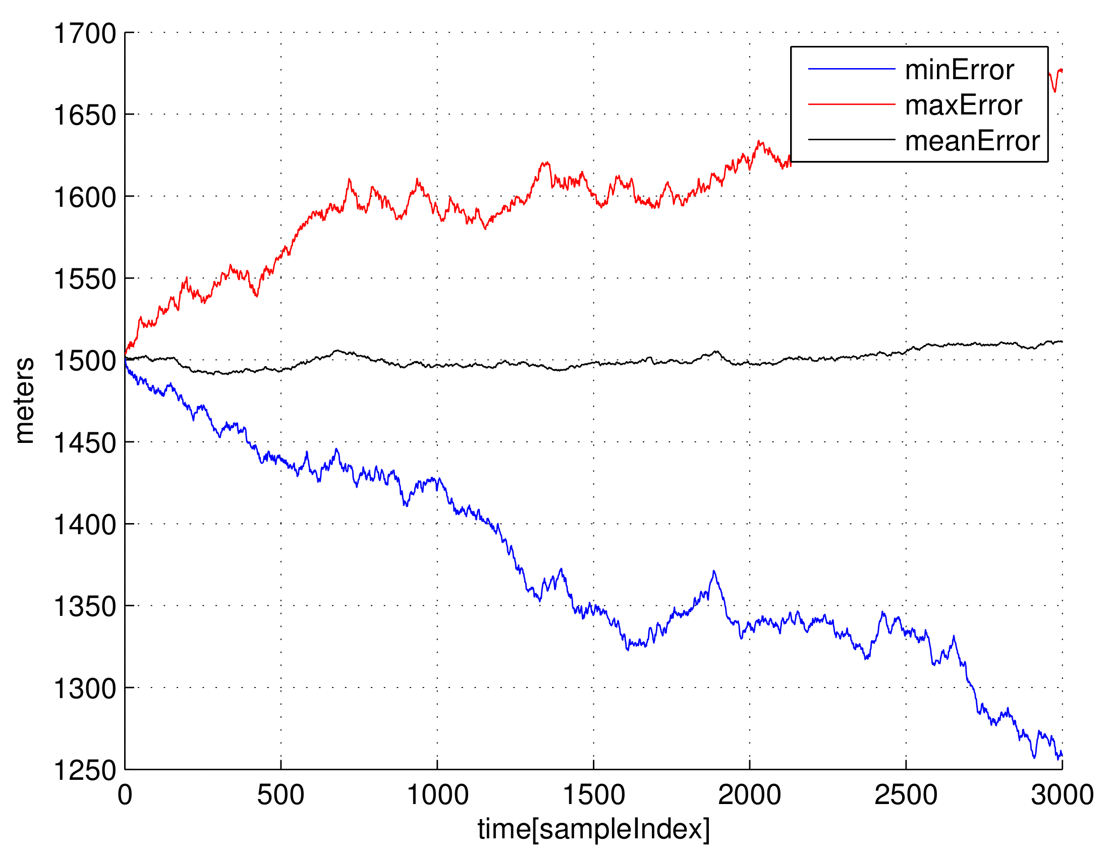
Consider the case where the IMU-only localization is used. In Figure 6, we plot , , and with respect to sample-index k. Since no ship is used to fix long-term drift, the estimation error does not decrease as time goes on. Compared to Figure 2 and Figure 4, the estimation error increases. To run one Monte-Carlo simulation takes only 0.6 seconds utilizing MATLAB simulations.
5. Conclusions
This paper presents the localization method of an AUV in environments, such as harbors or ports, where passing ships can exist. Assume that source levels and trajectories of the passing ships are known a priori. This paper introduces the AUV localization method based on bearing-only measurements of passing ships moving along known trajectories (planned routes). The RPEKF is used to reduce the range estimation error in bearing-only measurements.
As far as we know, this paper is novel in presenting the underwater localization method using RAM and sound measurements of ships moving along known routes. If we do not use the proposed localization, the AUV needs to depend on IMU-only localization. It is inevitable that the IMU-only localization leads to the integration of localization error as time goes on. The simulation results in Section 4.1 and Section 4.3 show that using the measurements of a single ship can improve the localization accuracy, compared to IMU-only localization.
Moreover, the simulation results in Section 4.1 and Section 4.2 show that using measurements from multiple ships gives better localization accuracy, compared to the case where the measurement of a single ship is used. As our future works, we will verify the effectiveness of the proposed localization method using experiments with a real AUV.
There may be a case where there exist many ships of the identical type (for example, container ships). In this case, it is not trivial to identify a ship by processing the sound of the ship. In the case where a ship is not correctly identified, we may generate false measurements, similar to clutters in BOTMA problems [43]. In the future, we will tackle the case where there exist many ships of the identical type.
The proposed localization scheme can be further applied for localization of various autonomous vehicles, such as an Unmanned Aerial Vehicle (UAV). The UAV can measure the directions of signals emitted from airplanes (or sites) of which trajectories (locations) are known a priori. Then, bearing direction measurements can be used for localization of the UAV. This localization scheme can be used when Global Positioning Systems are not available for the UAV.
Funding
This work was supported by the National Research Foundation of Korea (NRF) grant funded by the Korea government (MSIT) (No. 2019R1F1A1063151).
Conflicts of Interest
The author declares no conflict of interest.
References
- McKenna, M.F.; Ross, D.; Wiggins, S.M.; Hildebrand, J.A. Underwater radiated noise from modern commercial ships. J. Acoust. Soc. Am. 2012, 131, 92–103. [Google Scholar] [CrossRef] [PubMed] [Green Version]
- Tollefsen, D.; Dosso, S.E. Ship source level estimation and uncertainty quantification in shallow water via Bayesian marginalization. J. Acoust. Soc. Am. 2020, 147, 1–7. [Google Scholar] [CrossRef] [PubMed]
- Jiang, P.; Lin, J.; Sun, J.; Yi, X.; Shan, Y. Source spectrum model for merchant ship radiated noise in the Yellow Sea of China. Ocean Eng. 2020, 216, 1–13. [Google Scholar] [CrossRef]
- Gloza, I. Identification Methods of Underwater Noise Sources Generated by Small Ships. Acta Phys. Polonica A Acoust. Biomed. Eng. 2011, 119, 1–5. [Google Scholar] [CrossRef]
- Gonzalez-Garcia, J.; Gomez-Espinosa, A.; Cuan-Urquizo, E.; Garcia-Valdovinos, L.G.; Salgado-Jimenez, T.; Cabello, J.A.E. Autonomous Underwater Vehicles: Localization, Navigation, and Communication for Collaborative Missions. Appl. Sci. 2020, 10, 1256. [Google Scholar] [CrossRef] [Green Version]
- Rea, M.; Fakhreddine, A.; Giustiniano, D.; Lenders, V. Filtering Noisy 802.11 Time-of-Flight Ranging Measurements From Commoditized WiFi Radios. IEEE/ACM Trans. Netw. 2017, 25, 2514–2527. [Google Scholar] [CrossRef]
- Cheng, L.; Wu, C.; Zhang, Y.; Wu, H.; Li, M.; Maple, C. A Survey of Localization in Wireless Sensor Network. Int. J. Distrib. Sens. Netw. 2012, 2012, 962523. [Google Scholar] [CrossRef]
- Kim, J. Non-line-of-sight error mitigating algorithms for transmitter localization based on hybrid TOA/RSSI measurements. Wirel. Netw. 2020, 26, 3629–3635. [Google Scholar] [CrossRef]
- Howard, A.; Mataric, M.; Sukhatme, G. Relaxation on a mesh: A formalism for generalized localization. In Proceedings of the IEEE/RSJ International Conference on Intelligent Robots and Systems, Hawaii, HI, USA, 29 October–3 November 2001; pp. 1055–1060. [Google Scholar]
- Boccadoro, M.; Angelis, G.D.; Valigi, P. TDOA positioning in NLOS scenarios by particle filtering. Wirel. Netw. 2012, 18, 579–589. [Google Scholar] [CrossRef]
- Han, G.; Xu, H.; Duong, T.Q.; Jiang, J.; Hara, T. Localization algorithms of Wireless Sensor Networks: A survey. Telecommun. Syst. 2013, 52, 2419–2436. [Google Scholar] [CrossRef]
- Kim, J. Tracking a manoeuvring target while mitigating NLOS errors in TDOA measurements. IET Radar Sonar Navig. 2020, 14, 495–502. [Google Scholar] [CrossRef]
- Niculescu, D.; Nath, B. Ad hoc positioning system (APS) using AOA. In Proceedings of the Twenty-Second Annual Joint Conference of the IEEE Computer and Communications, San Francisco, CA, USA, 30 March–3 April 2003; pp. 1734–1743. [Google Scholar]
- Kim, J. Filter re-start strategy for angle-only tracking of a highly manoeuvrable target considering the target’s destination information. IET Radar Sonar Navig. 2020, 14, 935–943. [Google Scholar] [CrossRef]
- Almeida, J.; Matias, B.; Ferreira, A.; Almeida, C.; Martins, A.; Silva, E. Underwater Localization System Combining iUSBL with Dynamic SBL in VAMOS Trials. Sensors 2020, 20, 4710. [Google Scholar] [CrossRef]
- Costanzi, R.; Monnini, N.; Ridolfi, A.; Allotta, B.; Caiti, A. On field experience on underwater acoustic localization through USBL modems. In Proceedings of the OCEANS 2017—Aberdeen, Aberdeen, UK, 19–22 June 2017; pp. 1–5. [Google Scholar]
- Han, Y.; Zheng, C.; Sun, D. Accurate underwater localization using LBL positioning system. In Proceedings of the OCEANS 2015—MTS/IEEE Washington, Washington, DC, USA, 19–22 October 2015; pp. 1–4. [Google Scholar]
- Bahr, A.; Leonard, J.J.; Fallon, M.F. Cooperative Localization for Autonomous Underwater Vehicles. Int. J. Robot. Res. 2009, 28, 714–728. [Google Scholar] [CrossRef]
- Chen, Q.; You, K.; Song, S. Cooperative localization for autonomous underwater vehicles using parallel projection. In Proceedings of the 2017 13th IEEE International Conference on Control Automation (ICCA), Ohrid, Macedonia, 3–6 July 2017; pp. 788–793. [Google Scholar]
- Liu, J.; Wang, Z.; Peng, Z.; Cui, J.; Fiondella, L. Suave: Swarm underwater autonomous vehicle localization. In Proceedings of the IEEE INFOCOM 2014—IEEE Conference on Computer Communications, Toronto, ON, Canada, 27 April–2 May 2014; pp. 64–72. [Google Scholar]
- Xu, B.; Li, S.; Razzaqi, A.A.; Zhang, J. Cooperative Localization in Harsh Underwater Environment Based on the MC-ANFIS. IEEE Access 2019, 7, 55407–55421. [Google Scholar] [CrossRef]
- Cao, Y.; Ren, W.; Egerstedt, M. Distributed Containment Control with Multiple Stationary or Dynamic Leaders in Fixed and Switching Directed Networks. Automatica 2012, 48, 1586–1597. [Google Scholar] [CrossRef]
- Zhao, S.; Chen, B.M.; Lee, T.H. Optimal placement of bearing-only sensors for target localization. In Proceedings of the 2012 American Control Conference (ACC), Montreal, QC, Canada, 27–29 June 2012; pp. 5108–5113. [Google Scholar]
- Moreno-Salinas, D.; Pascoal, A.; Aranda, J. Sensor Networks for Optimal Target Localization with Bearings-Only Measurements in Constrained Three-Dimensional Scenarios. Sensors 2013, 13, 10386–10417. [Google Scholar] [CrossRef] [PubMed] [Green Version]
- Bayat, M.; Crasta, N.; Aguiar, A.P.; Pascoal, A.M. Range-Based Underwater Vehicle Localization in the Presence of Unknown Ocean Currents: Theory and Experiments. IEEE Trans. Control Syst. Technol. 2016, 24, 122–139. [Google Scholar] [CrossRef]
- Allotta, B.; Costanzi, R.; Fanelli, F.; Monni, N.; Paolucci, L.; Ridolfi, A. Sea currents estimation during AUV navigation using Unscented Kalman Filter. IFAC PapersOnLine 2017, 50, 13668–13673. [Google Scholar] [CrossRef]
- Allotta, B.; Caiti, A.; Costanzi, R.; Di Corato, F.; Fenucci, D.; Monni, N.; Pugi, L.; Ridolfi, A. Cooperative navigation of AUVs via acoustic communication networking: Field experience with the Typhoon vehicles. Autonomous Robot 2016, 40, 1229–1244. [Google Scholar] [CrossRef]
- Medagoda, L.; Kinsey, J.C.; Eilders, M. Autonomous Underwater Vehicle localization in a spatiotemporally varying water current field. In Proceedings of the 2015 IEEE International Conference on Robotics and Automation (ICRA), Seattle, WA, USA, 26–30 May 2015; pp. 565–572. [Google Scholar]
- Hsieh, H.W.; Lee, C.L.; Kuo, C.L. Localization of an underwater robot with inertial sensor fusion models. In Proceedings of the 2010 5th IEEE Conference on Industrial Electronics and Applications, Taichung, Taiwan, 15–17 June 2010; pp. 1562–1567. [Google Scholar]
- Melim, A.; West, M. Towards autonomous navigation with the Yellowfin AUV. In Proceedings of the OCEANS’11 MTS/IEEE KONA, Waikoloa, HI, USA, 19–22 September 2011; pp. 1–5. [Google Scholar]
- Corke, P.; Detweiler, C.; Dunbabin, M.; Hamilton, M.; Rus, D.; Vasilescu, I. Experiments with Underwater Robot Localization and Tracking. In Proceedings of the 2007 IEEE International Conference on Robotics and Automation, Roma, Italy, 10–14 April 2007; pp. 4556–4561. [Google Scholar]
- Kim, J.; Suh, T.; Ryu, J. Bearings-only target motion analysis of a highly manoeuvring target. IET Radar Sonar Navig. 2017, 11, 1011–1019. [Google Scholar] [CrossRef]
- Fei, Z.; Zhou, X.P.; Chen, X.H.; Liu, R.L. Particle Filter for Underwater Bearings-Only Passive Target Tracking. In Proceedings of the 2008 IEEE Pacific-Asia Workshop on Computational Intelligence and Industrial Application, Washington, DC, USA, 19–20 December 2008; Volume 2, pp. 847–851. [Google Scholar]
- Ristic, B.; Arulampalam, S.; Gordon, N. Beyond the Kalman Filter: Particle Filters for Tracking Applications; Artech House: Norwood, MA, USA, 2004. [Google Scholar]
- Kim, J. Maneuvering target tracking of underwater autonomous vehicles based on bearing-only measurements assisted by inequality constraints. Ocean Eng. 2019, 189, 106404. [Google Scholar] [CrossRef]
- Nardone, S.C.; Aidala, V.J. Observability Criteria for Bearings-Only Target Motion Analysis. IEEE Trans. Aerospace Electron. Syst. 1981, AES-17, 162–166. [Google Scholar] [CrossRef]
- Karlsson, R.; Gustafsson, F. Recursive Bayesian estimation: Bearing-only applications. IEE Proc. Radar Sonar Navig. 2005, 152, 305–313. [Google Scholar] [CrossRef] [Green Version]
- Peach, N. Bearings-only tracking using a set of range-parameterised extended Kalman filters. IEE Proc. Control Theory Appl. 1995, 142, 73–80. [Google Scholar] [CrossRef]
- Collins, M.D. User’s Guide for RAM Versions 1.0 and 1.0p; Naval Research Laboratory: Washington, DC, USA, 1995. [Google Scholar]
- Collins, M.D. A split-step Pade solution for the parabolic equation method. J. Acoust. Soc. Am. 1993, 93, 1736–1742. [Google Scholar] [CrossRef]
- Jensen, F.B.; Kuperman, W.A.; Porter, M.B.; Schmidt, H. Computational Ocean Acoustics; Springer: New York, NY, USA, 2011. [Google Scholar]
- Urick, R.J. Principles of Underwater Sound; McGraw-Hill: New York, NY, USA, 1983. [Google Scholar]
- Li, X.; Zhao, C.; Lu, X.; Wei, W. Underwater Bearings-Only Multitarget Tracking Based on Modified PMHT in Dense-Cluttered Environment. IEEE Access 2019, 7, 93678–93689. [Google Scholar] [CrossRef]
Figure 1.
The AUV starts from the origin. The ship starts from (2000,0) in meters, and the trajectory of the ship at every minute is plotted with red asterisks. The starting point of the ship is marked with a diamond. At every minute, the trajectory of the AUV is depicted with blue circles (one ship scenario).

Figure 2.
Consider the case where the proposed localization method is utilized. We plot , , and with respect to sample-index k. The AUV maneuvers at 750 and 2250 s. At these moments, the estimation error decreases sharply. This is similar to the case where the maneuver of an observer makes the Bearing-Only Target Motion Analysis (BOTMA) system observable [36].

Figure 3.
The AUV starts from the origin. The starting point of each ship is marked with a diamond. At every minute, the trajectory of every ship is plotted with red asterisks. At every minute, the trajectory of the AUV is depicted with blue circles (three ships scenario).
Figure 3.
The AUV starts from the origin. The starting point of each ship is marked with a diamond. At every minute, the trajectory of every ship is plotted with red asterisks. At every minute, the trajectory of the AUV is depicted with blue circles (three ships scenario).

Figure 4.
Consider the case where the proposed localization method is utilized. We plot , , and with respect to sample-index k. See that the estimation error decreased considerably, compared to Figure 2. This is due to the fact that the AUV localization uses three bearing lines emitted from three ships, instead of one bearing line emitted from one ship. (three ships scenario).

Figure 5.
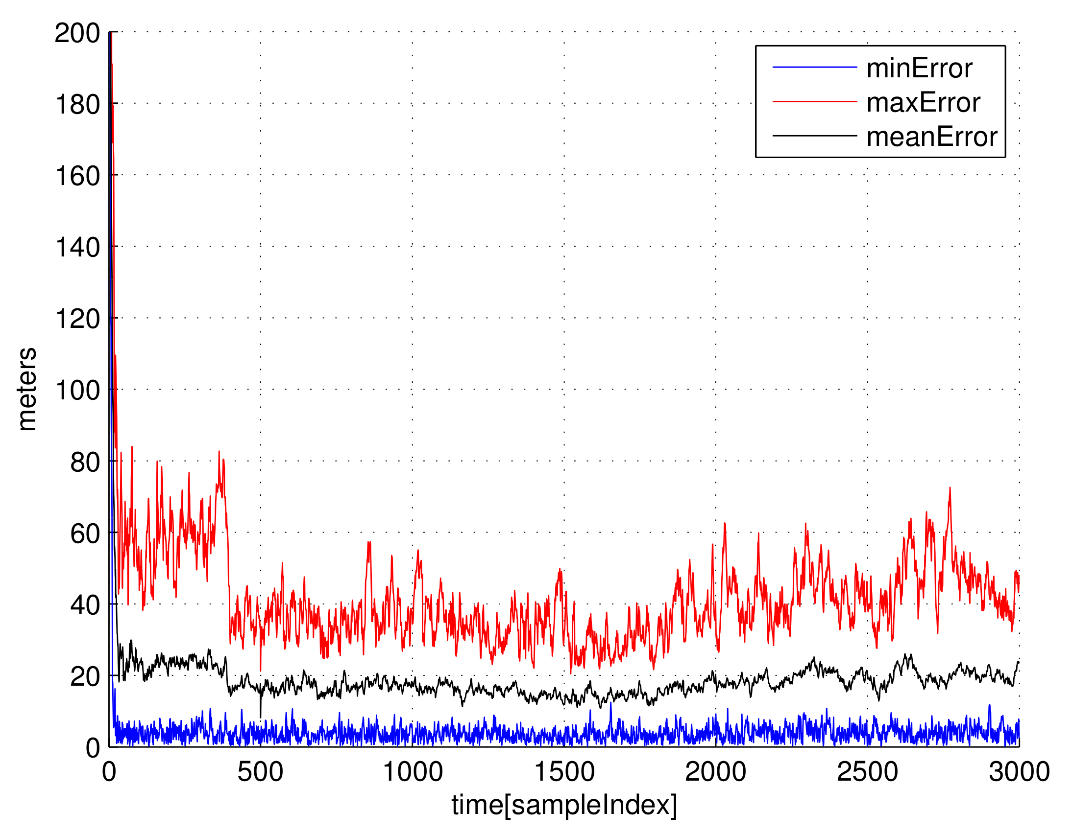
The enlarged figure of Figure 4. We plot , , and with respect to sample-index k. Since we utilize the bearing measurements of three ships, the estimation error is small from the beginning of the scenario (three ships scenario).
Figure 5.
The enlarged figure of Figure 4. We plot , , and with respect to sample-index k. Since we utilize the bearing measurements of three ships, the estimation error is small from the beginning of the scenario (three ships scenario).

Figure 6.
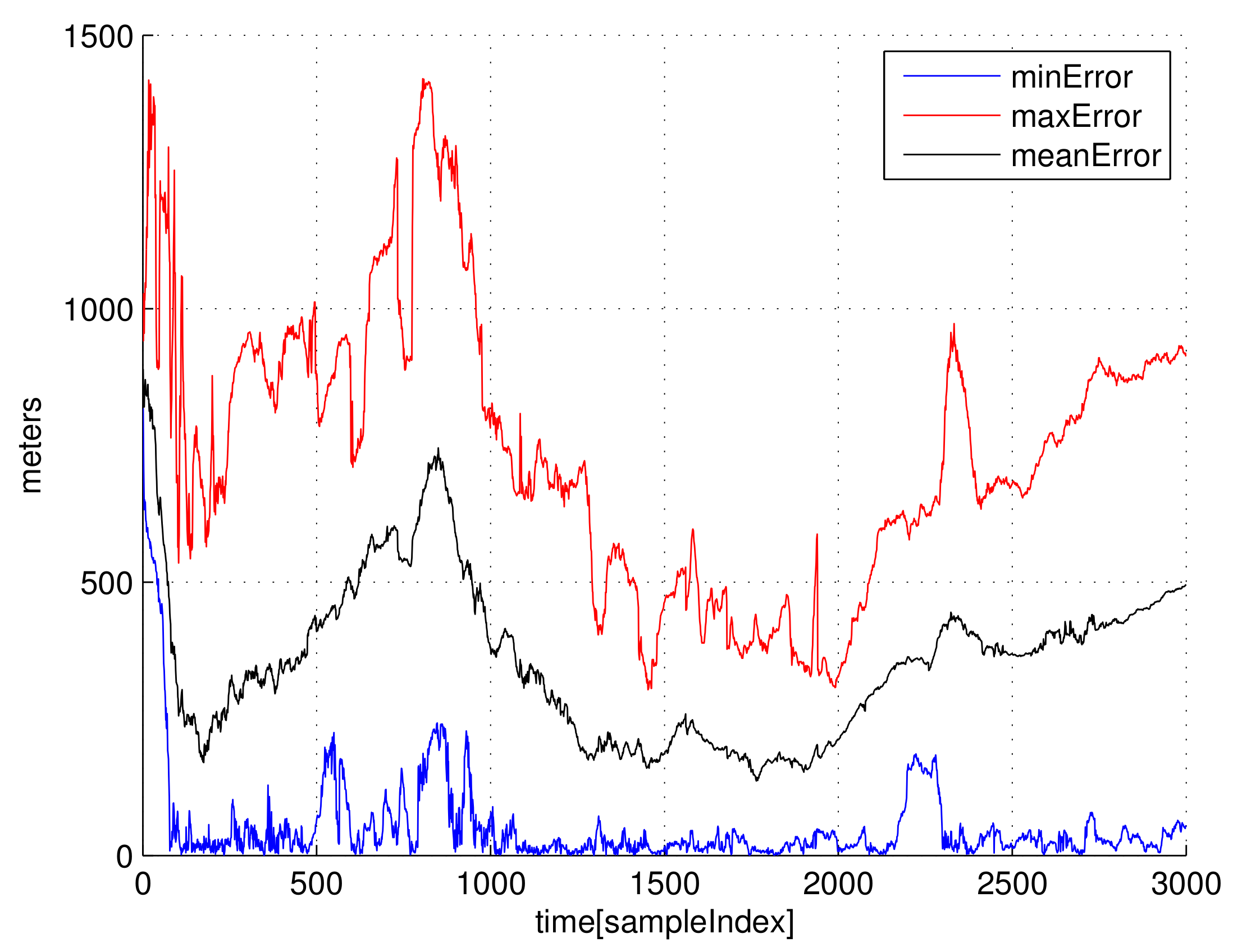
Consider the case where the Inertial Measurement Units (IMU)-only localization is used. We plot , , and with respect to sample-index k. Since no ship is used to fix long-term drift, the estimation error does not decrease as time goes on. Compared to Figure 2 and Figure 4, the estimation error increases.
Figure 6.
Consider the case where the Inertial Measurement Units (IMU)-only localization is used. We plot , , and with respect to sample-index k. Since no ship is used to fix long-term drift, the estimation error does not decrease as time goes on. Compared to Figure 2 and Figure 4, the estimation error increases.

Publisher’s Note: MDPI stays neutral with regard to jurisdictional claims in published maps and institutional affiliations. |
© 2020 by the author. Licensee MDPI, Basel, Switzerland. This article is an open access article distributed under the terms and conditions of the Creative Commons Attribution (CC BY) license (http://creativecommons.org/licenses/by/4.0/).
Share and Cite
MDPI and ACS Style
Kim, J. Autonomous Underwater Vehicle Localization Using Sound Measurements of Passing Ships. Appl. Sci. 2020, 10, 9139. https://doi.org/10.3390/app10249139
AMA Style
Kim J. Autonomous Underwater Vehicle Localization Using Sound Measurements of Passing Ships. Applied Sciences. 2020; 10(24):9139. https://doi.org/10.3390/app10249139
Chicago/Turabian StyleKim, Jonghoek. 2020. "Autonomous Underwater Vehicle Localization Using Sound Measurements of Passing Ships" Applied Sciences 10, no. 24: 9139. https://doi.org/10.3390/app10249139
Note that from the first issue of 2016, this journal uses article numbers instead of page numbers. See further details here.