Modeling and Speed Tuning of a PMSM with Presence of Fissure Using Dragonfly Algorithm

 and
and
Abstract
:1. Introduction
2. Dynamic PMSM Model with Presence of Rotor Fissure
2.1. Fracture Dynamics in the Rotor Shaft
2.2. Dynamic Coupled Model
3. Reference Model
3.1. Desired Behavior of the Error
3.2. Optimal Linear Quadratic Control for States ,
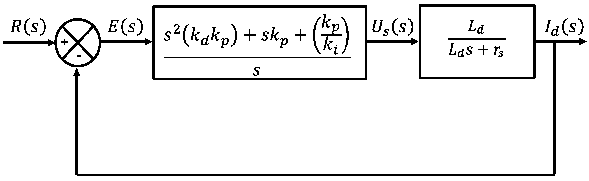
3.3. PID Controller for id Current
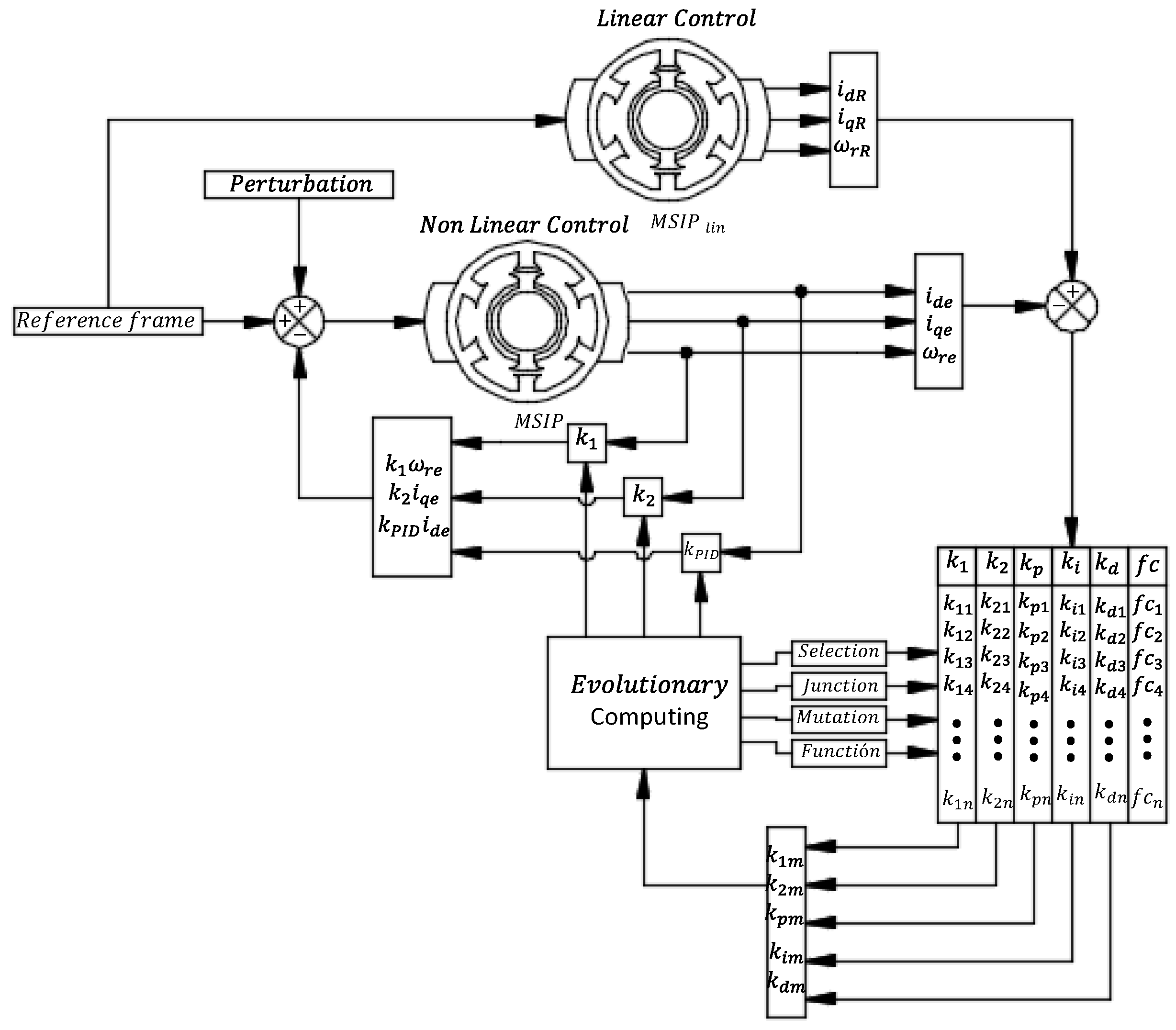
4. Tuning of Controller Using the Dragonfly Algorithms
| Algorithm 1 Dragonfly Algorithm |
| Define population size (M) |
| begin the iteration counter |
| Initialize the population by generating for |
| Calculate the objective function values of all dragonflies |
| Update the food and the predator’s location |
| while (the stop criterion is not satisfied) do |
| for |
| Update neighborhood radius (or update w, s, a, c, f, and e) |
| if a dragonfly has at least one neighborhood dragonfly |
| Separation motion |
| Alignment motion |
| Cohesion motion |
| Food attraction motion |
| Predator distraction motion |
| else |
| Update position vector using the Lévy flight function |
| end if |
| end for i |
| Sort the population/dragonflies from best to and find the current best |
| end while |
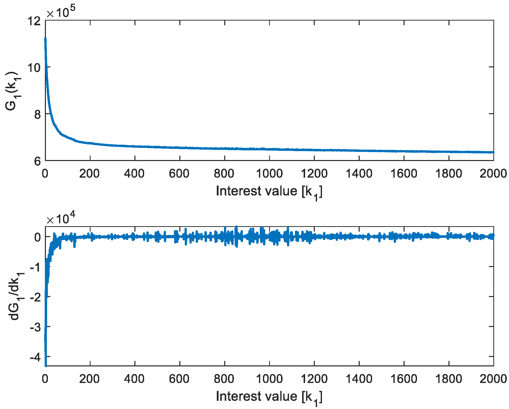
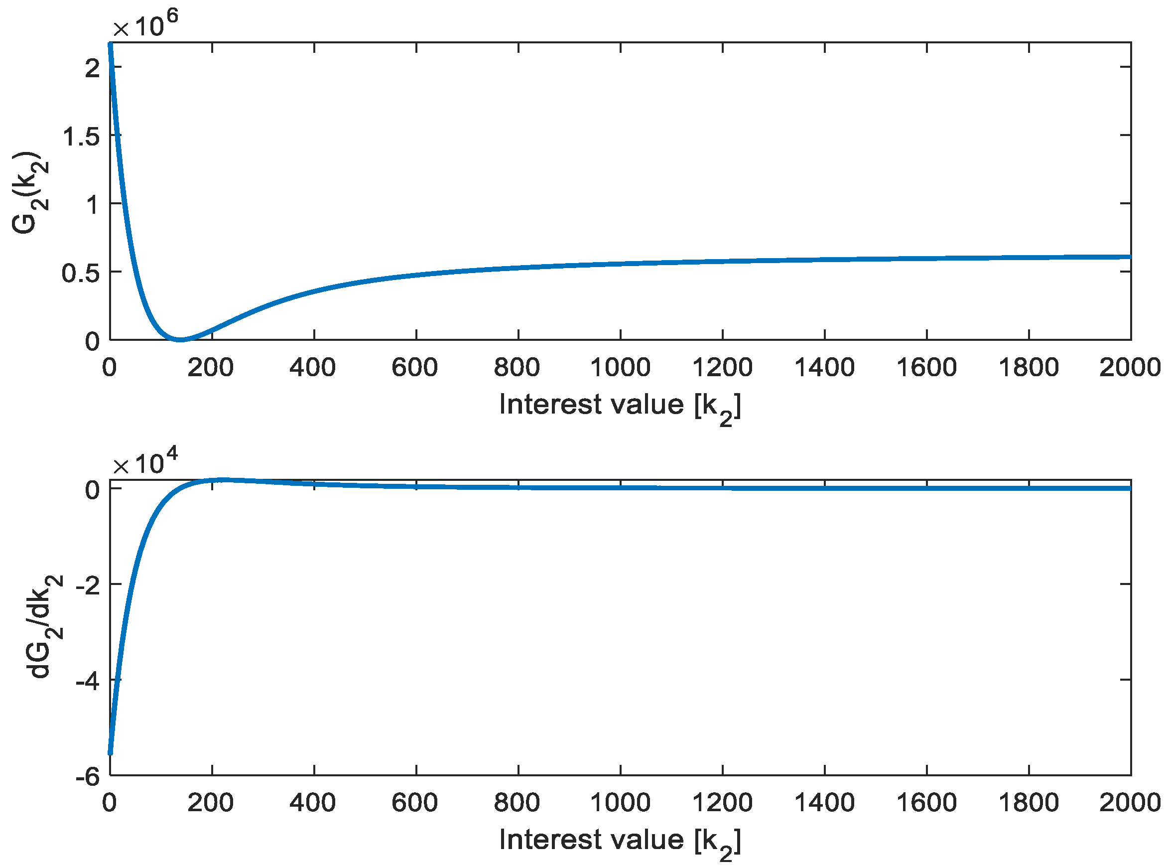
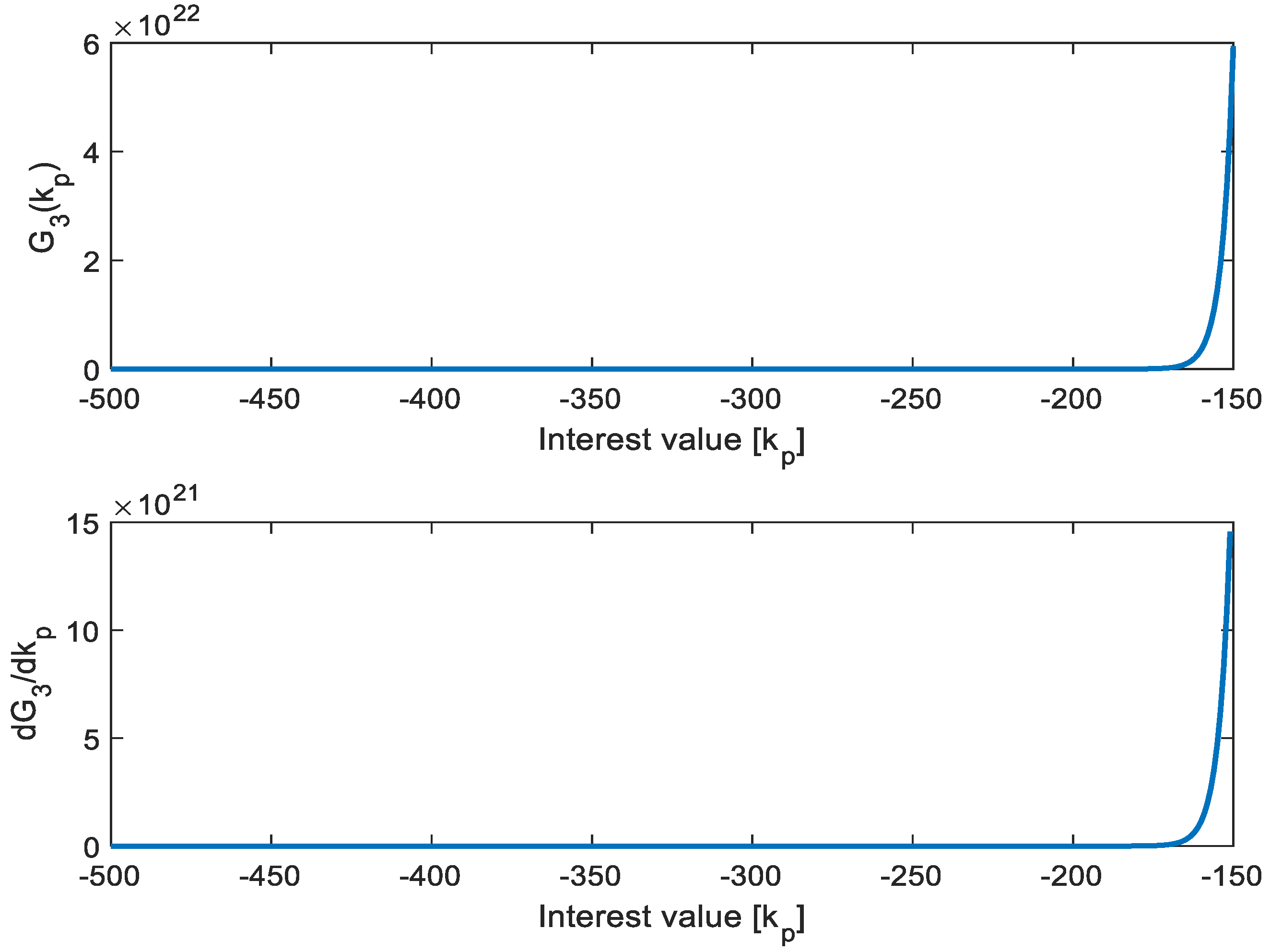
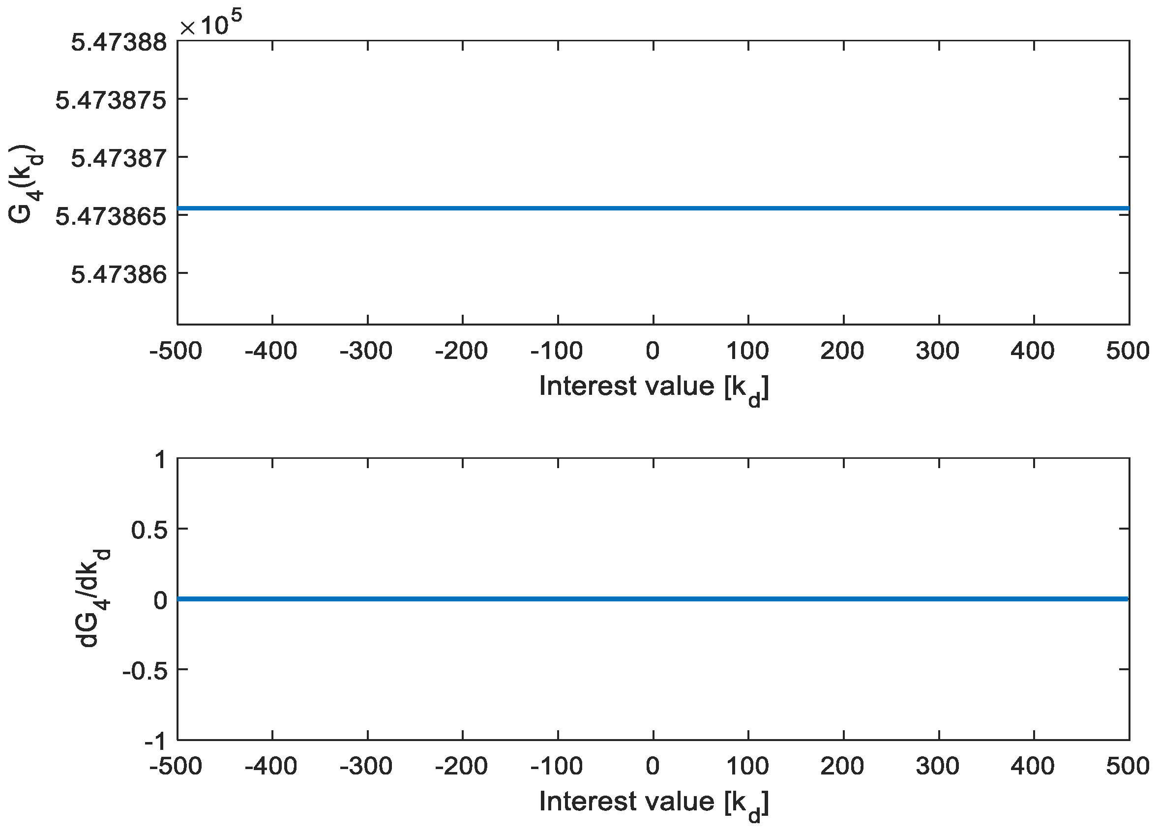
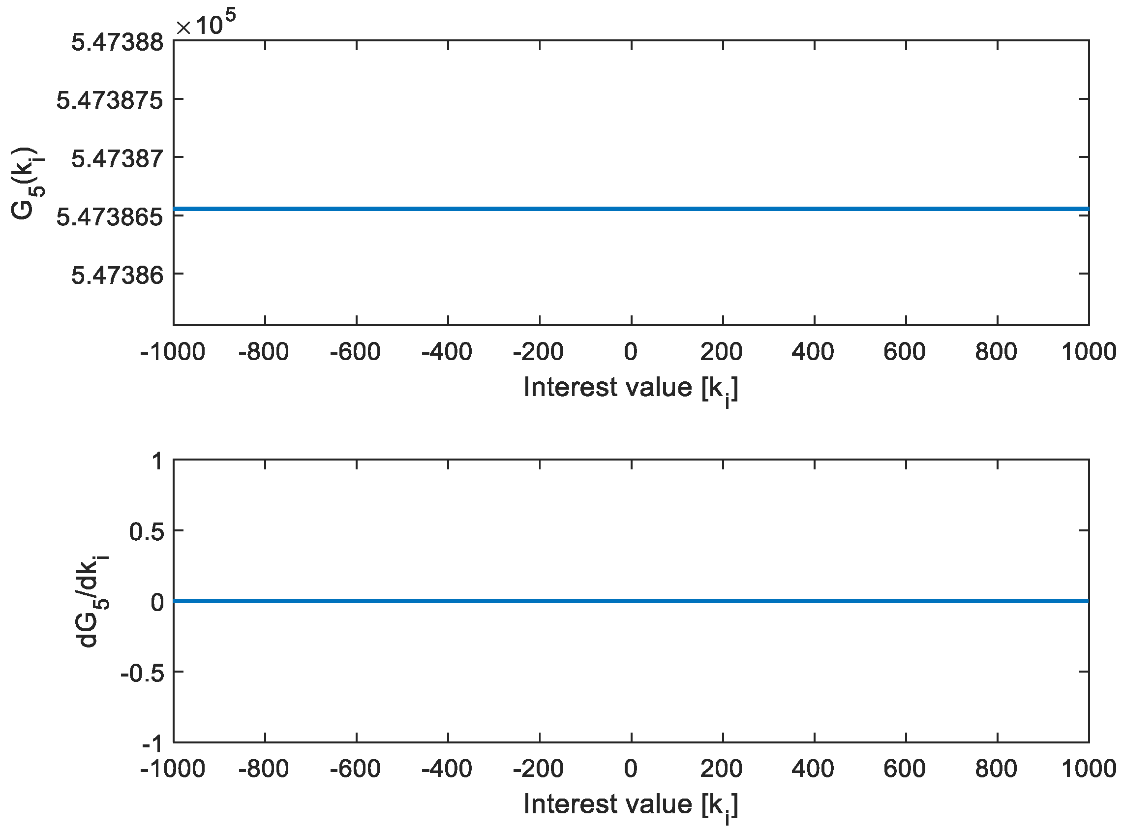
5. Sensitivity Analysis
6. Simulation
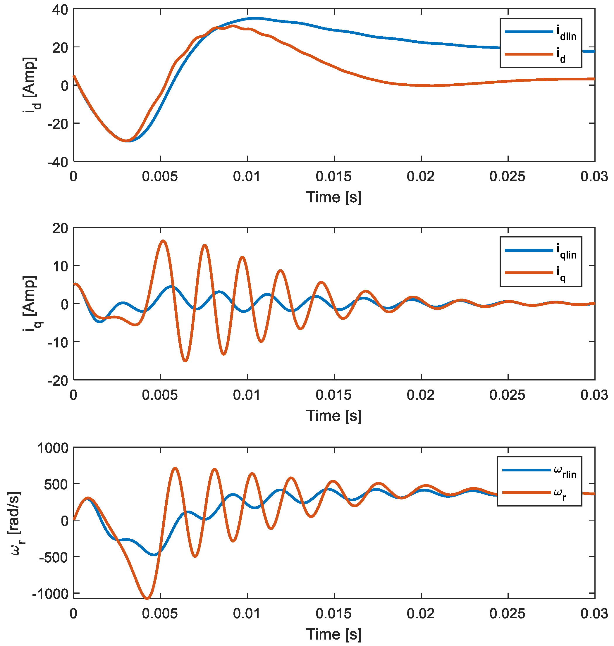
7. Results
8. Conclusions
Author Contributions
Funding
Acknowledgments
Conflicts of Interest
Nomenclature
| Parameters | Definition |
| Stator currents in the rotating dq reference frame | |
| Angular position of the rotor shaft | |
| Angular speed of the rotor | |
| a | Fissure size |
| Stator voltages in the rotating dq reference frame | |
| Stator inductances on the dq reference axes | |
| Stator phase resistance | |
| P | Number of pole pairs |
| J | Polar moment of inertia |
| Rotor mass | |
| Rotational inertia dependent on fissure size | |
| Permanent magnetic flow | |
| f | Fundamental rotor frequency |
| β | Viscous damping coefficient |
| c | Proportional coefficient (material dependent) |
| n | Proportional exponent (material dependent) |
| D | Root of rotor shaft diameter |
| External load torque | |
| Electric torque (generated by the motor) | |
| g | Mayes and Davis fissure respite function |
| d | Diameter of the hole in the rotor shaft due to the fissure |
| Variation of the stress concentrator | |
| Torsional stress variation in the rotor shaft | |
| Initial model conditions | |
| Nominal value of the voltage applied in phases dq | |
| Electric angular displacement | |
| System Status Errors | |
| Desired error coefficient | |
| Desired values of system states | |
| Q, R | Hermetic Matrices of optimal control |
| X | Vector of linear quadratic optimal control states |
| System control inputs | |
| Linear Quadratic Optimal Control Gains | |
| Gains from Proportional Integral and Derivative Control (PID) | |
| PID Controller Profit Locating Roots | |
| Linear Quadratic Optimum Controller Power | |
| Total energy of the PMSM dynamic system | |
| PMSM kinetic energy | |
| PMSM potential energy | |
| G | Energy cost of the PMSM dynamic system |
| PMSM dynamic system sensitivity | |
| Cost localization function of optimal earnings | |
| Optimal earnings vector | |
| Value obtained from the jth search for speed gain |
References
- Gieras, J.F.; Wing, M. Permanent Magnet Motor Technology: Desing and Applications, 2nd ed.; Marcel Dekker: New York, NY, USA, 2002; pp. 1–15a, 169–187b. [Google Scholar]
- Quiroz, J.C.; Maurin, N.; Rezazadeh, M.; Izadi, M.; Misron, N. Fault detection of broken rotor bar in LS-PMSM using random forests. Measurement 2018, 116, 273–280. [Google Scholar] [CrossRef]
- Bachschmid, N.; Pennacchi, P.; Tanzi, E. Cracker Rotors; Springer: Berlin, Germany, 2010; pp. 4–14. [Google Scholar]
- Harzelli, I.; Menacer, A.; Ameid, T. A fault monitoring approach using model-based and neural network techniques applied to input–output feedback linearization control induction motor. J. Ambient. Intell. Human. Comput. 2020, 11, 2519–2538. [Google Scholar] [CrossRef]
- Nath, A.G.; Udmale, S.S.; Singh, S.K. Role of artificial intelligence in rotor fault diagnosis: A comprehensive review. Artif. Intell. Rev. 2020. [Google Scholar] [CrossRef]
- Liu, G.; Mao, K. A Novel Power Failure Compensation Control Method for Active Magnetic Bearings Used in High-Speed Permanent Magnet Motor. IEEE Trans. Power Electron. 2016, 31, 4565–4575. [Google Scholar] [CrossRef]
- Gangsar, P.; Tiwari, R. Diagnostics of mechanical and electrical faults in induction motors using wavelet-based features of vibration and current through support vector machine algorithms for various operating conditions. J. Braz. Soc. Mech. Sci. Eng. 2019, 41, 71. [Google Scholar] [CrossRef]
- Al-Bedoor, B.O.; Moustafa, K.A.; Al-Hussain, K.M. Predicting the fatigue life of synchronous motor-driven compressor using the complex modal reduction technique. Comput. Methods Appl. Mech. Eng. 2000, 187, 53–68. [Google Scholar] [CrossRef]
- Mekki, H.; Benzineb, O.; Boukhetala, D.; Chrifi-Alaoui, L.; Tadjine, M. Fault Tolerant Design for Permanent Magnet Synchronous Motor using Fuzzy Speed Controller. IFAC-PapersOnLine 2016, 49, 315–320. [Google Scholar] [CrossRef]
- Villalobos-Piña, F.; Alvarez-Salas, R. Algoritmo robusto para el diagnóstico de fallas eléctricas en motor de inducción trifásico basado en herramientas espectrales y ondeletas. Rev. Iberoam. Automática Inf. Ind. 2015, 12, 292–303. [Google Scholar] [CrossRef] [Green Version]
- Guha, D.; Roy, P.K.; Banerjee, S. Optimal tuning of 3 degree-of-freedom proportional-integral-derivative controller for hybrid distributed power system using dragonfly algorithm. Comput. Electr. Eng. 2018, 72, 137–153. [Google Scholar] [CrossRef]
- Simhadri, K.; Mohanty, B.; Mohan, R. Optimized 2DOF PID for AGC of Multi-area Power System Using Dragonfly Algorithm. In Applications of Artificial Intelligence Techniques in Engineering; Malik, H., Srivastava, S., Sood, Y., Ahmad, A., Eds.; Springer: Singapore, 2019; pp. 11–22. [Google Scholar] [CrossRef]
- Xue, W.; Li, Y.; Cang, S.; Jia, H.; Wang, Z. Chaotic behavior and circuit implementation of a fractional-order permanent magnet synchronous motor model. J. Frankl. Inst. 2015, 2887–2898. [Google Scholar] [CrossRef]
- Venkatesan, K.; Liu, Y. Subcycle fatigue crack growht formulation under positive and negative stress ratios. Eng. Fract. Mech. 2018, 189, 390–404. [Google Scholar] [CrossRef]
- Andrade, A.A.; Mosquera, W.A.; Vanegas, L.V. Modelos de crecimiento de grietas por fatiga. Entre Cienc. Ing. 2015, 9, 39–48. [Google Scholar] [CrossRef]
- Arana, J.L.; González, J.J. Mecánica de la Fractura; Servicio Editorial de la Universidad del País Vasco: Leioa, Spain, 2011; p. 186. [Google Scholar]
- Barter, S.; White, P.; Burchill, M. Fatigue Crack path manipulation for crack growth rate measurement. Eng. Fract. Mech. 2016, 167, 224–238. [Google Scholar] [CrossRef]
- Genta, G. Dynamics of Rotating System; Springer: Berlin, Germany, 2005; pp. 332–354. [Google Scholar]
- Rasoolzadeh, A.; Tavazoei, M.S. Prediction of chaos in non-salient permanentmagnet synchronous machines. Phys. Lett. A 2012, 73–79. [Google Scholar] [CrossRef]
- Krishnan, R. Permanent Magnet Synchronous and Brushless DC Motor Drives; CRC Press: Boca Raton, FL, USA, 2010; pp. 225–276. [Google Scholar]
- Aguilar-Mejía, O.; Tapia–Olvera, R.; Valderrabano-González, A.; Rivas-Cambero, I. Adaptive neural network control of chaos in permanent magnet synchronous motor, Taylor and Francis Group. Intell. Autom. Soft Comput. 2015, 22, 499–507. [Google Scholar] [CrossRef]
- Xu, W.J. Permanent Magnet Synchronous Motor with Linear Quadratic Speed Controller. Energy Procedia 2011, 14, 364–369. [Google Scholar] [CrossRef] [Green Version]
- Yun-Jie, W.; Guo-Fei, L. Adaptive disturbance compensation finite control set optimal control for PMSM systems based on sliding mode extended state observer. Mech. Syst. Signal. Process. 2018, 98, 402–414. [Google Scholar] [CrossRef]
- Meraihi, Y.; Ramdane-Cherif, A.; Acheli, D.; Mahseur, M. Dragonfly algorithm: A comprehensive review and applications. Neural Comput. Appl. 2020, 32, 16625–16646. [Google Scholar] [CrossRef]
- Mirjalili, S. Dragonfly algorithm: A new meta-heuristic optimization technique for solving single-objective, discrete, and multi-objective problems. Neural Comput. Appl. 2016, 27, 1053–1073. [Google Scholar] [CrossRef]
- Boroni, G.; Lotito, P.; Clausse, A. Análisis de sensibilidad de sistemas algebraicos diferenciales. Asoc. Argent. Mecánica Comput. 2006, 25, 1071–1085. [Google Scholar]
- Krauze, P.; Wasynczuk, O.; Sudhoff, S.; Pekarek, S. Analysis of Electric Machinery and Drive Systems, 3rd ed.; IEEE Press: Hoboken, NJ, USA, 2013; pp. 191–256. [Google Scholar]


| Parameters | Numerical Value | Units |
|---|---|---|
| 6.73 | Inductance [mH] | |
| 6.73 | Inductance [mH] | |
| 2.6 | Resistance [Ω] | |
| P | 4 | Pairs of poles |
| J | 3.5 × 10⁻⁵ | Rotational inertia [kgm2] |
| 0.1 | Rotor mass [kg] | |
| 0.319 | Magnetic flux [Wb] | |
| f | Frequency [Hz] | |
| β | 5 × 10⁻⁵ | |
| c | 10 × 10−11 | Proportional coefficient |
| n | 3 | Proportional exponent |
| D | 0.137409 | Root of rotor diameter [m1/2] |
| 5 | Load torque | |
| 0 | Initial current d | |
| 0 | Initial current q | |
| 0 | Initial angular velocity [rad/s] | |
| 0 | Initial angular position [rad] | |
| 3 × 10⁻⁸ | Initial fissure size [m] | |
| 90 | Nominal Voltage [V] | |
| 1500.5 | ||
| 188.5 | Desired angular velocity [rad/s] | |
| −1 | Desired Root 1 | |
| −1 | Desired Root 2 |
| Parameters | Numerical Value |
|---|---|
| Population size | 40 |
| Maximum of iteration | 100 |
| Random values | r1 = r2 = [0; 1] |
| Separation weight | 0.12 |
| Alignment weight | 0.12 |
| Cohesion weight | 0.75 |
| Food factor | 1 |
| Enemy factor | 1 |
| Inertia weight | 0.9–0.2 |
| β | 1.5 |
Publisher’s Note: MDPI stays neutral with regard to jurisdictional claims in published maps and institutional affiliations. |
© 2020 by the authors. Licensee MDPI, Basel, Switzerland. This article is an open access article distributed under the terms and conditions of the Creative Commons Attribution (CC BY) license (http://creativecommons.org/licenses/by/4.0/).
Share and Cite
Aguilar-Mejía, O.; Manilla-García, A.; Rivas-Cambero, I.; Minor-Popocatl, H. Modeling and Speed Tuning of a PMSM with Presence of Fissure Using Dragonfly Algorithm. Appl. Sci. 2020, 10, 8823. https://doi.org/10.3390/app10248823
Aguilar-Mejía O, Manilla-García A, Rivas-Cambero I, Minor-Popocatl H. Modeling and Speed Tuning of a PMSM with Presence of Fissure Using Dragonfly Algorithm. Applied Sciences. 2020; 10(24):8823. https://doi.org/10.3390/app10248823
Chicago/Turabian StyleAguilar-Mejía, Omar, Abraham Manilla-García, Ivan Rivas-Cambero, and Hertwin Minor-Popocatl. 2020. "Modeling and Speed Tuning of a PMSM with Presence of Fissure Using Dragonfly Algorithm" Applied Sciences 10, no. 24: 8823. https://doi.org/10.3390/app10248823