Dynamic Energy Modelling as an Alternative Approach for Reducing Performance Gaps in Retrofitted Schools in Denmark

Abstract

When considering that over 80% of buildings in Denmark were built before the 1980′s, a holistic energy retrofitting of the existing building stock is a major milestone to attain the energy and environmental targets of the country. In this work, a case study of three public schools is considered for post-retrofit process evaluation. The three schools were heavily retrofitted by September 2018 with energy conservation and improvement measures that were implemented targeting both the building envelope and various energy systems. A technical evaluation of the energy retrofit process in the schools was carried out, when considering one year of operation after the completion of the retrofitting work. Actual data from the heating and electricity meters in the schools were collected and compared with the pre-retrofit design numbers which rely majorly on static tabulated numbers for savings evaluation. It was shown that the retrofit design numbers largely overestimate the attained savings, where the average performance gap between the expected and real numbers for the three schools is around 61% and 136% for annual heating and electricity savings, respectively. On the other hand, an alternative approach was proposed where calibrated dynamic energy performance models, which were developed for the three schools in EnergyPlus, were used to simulate the impact of implementing the retrofit measures. It was shown that implementing this approach could predict much better the impacts of the retrofit process with an average gap of around 17% for heating savings and 21% for electricity savings. Based on the post-retrofit process evaluation in the three schools, it was concluded that using dynamic model simulations has the potential of lowering the performance gap between the promised and real savings when compared to static tabulated approaches, although the savings are still generally over-estimated in both approaches.

1. Introduction

1.1. Background

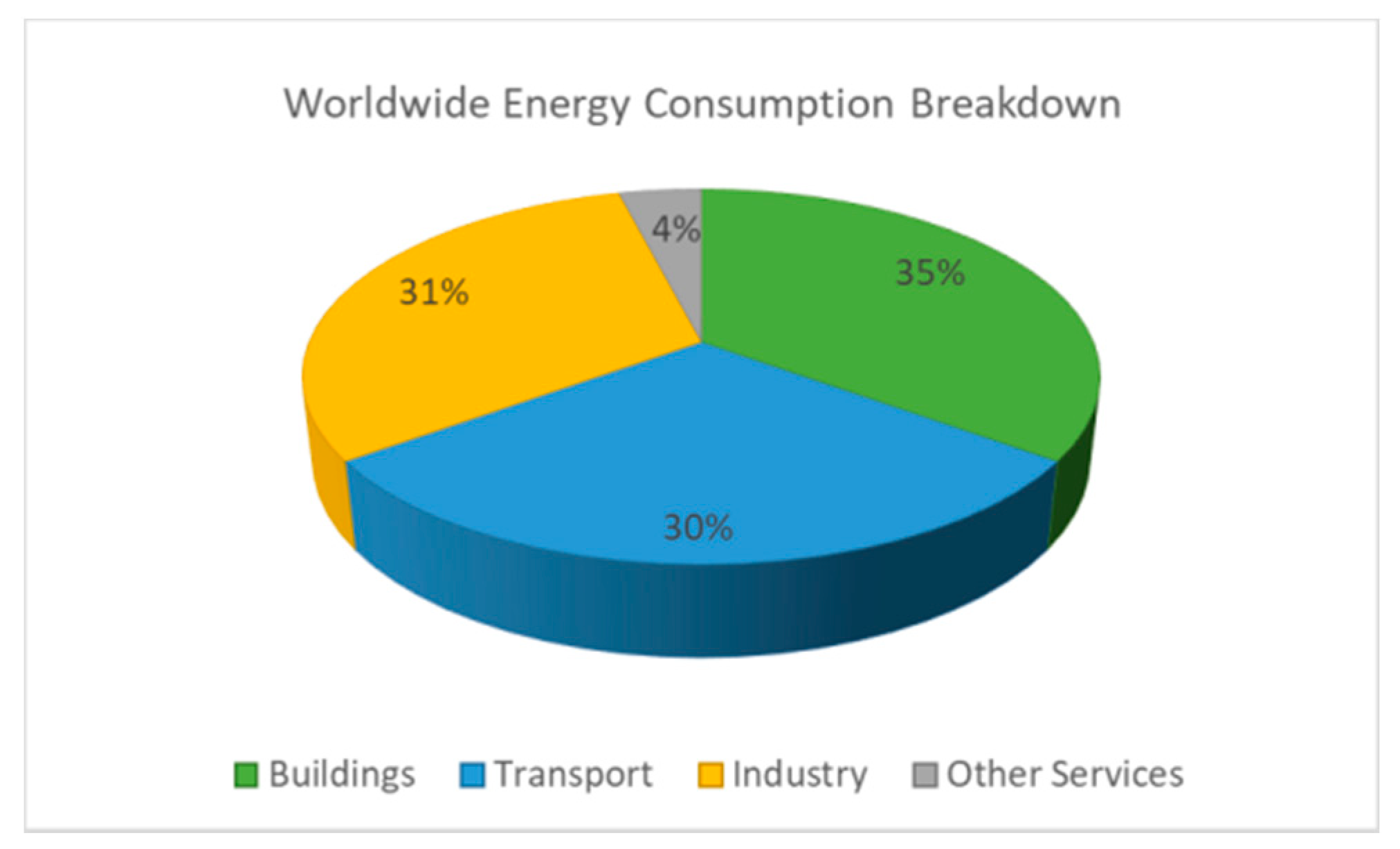
When considering the worldwide final energy consumption by sector, Figure 1 shows that the buildings sector is the largest consumer, with a share of around 35% of the overall energy consumption [1], more than the transport and industry sectors contribution. With the high rate of global urbanization levels along with the technological advancement and modernization, the buildings energy consumption share, including both commercial and residential buildings, is also expected to steadily increase by 50% until 2050 as compared to 2013 numbers [2]. In particular, buildings consume around 40% of the overall EU and US energy consumption, with a corresponding CO₂ emissions share of 36% [3]. In recent decades, the EU has considered the building sector as a priority, aiming to achieve the ambitious 2020 and 2050 goals. Thus, huge efforts have been devoted by EU member states to improve the overall energy performance of buildings, and the 2002 and 2010 EU Energy Performance of Building Directive [4] set strict requirements for enhancing the buildings energy efficiency. It was highlighted that around 30% energy savings potential could be achieved in 2020 through a comprehensive and systematic energy retrofit processes. Nevertheless, aiming to improve building energy management and optimizing the operation of building systems, the EU Directive 2018/844 [5] of the EU Parliament has set strict requirements regarding installing and assessing Building Management Systems (BMS) in public and commercial buildings in the member states.

1.2. Building Peformance Gap

The majority of the recent building standards and regulations in different countries have targeted improving the design and the energy performance of newly built energy efficient buildings. In addition, the absence of building continuous commissioning and performance monitoring have been reported as a major challenge facing the building stock and leading to energy performance gaps between the predicted and actual measured performance [6]. In the recent two decades, a large block of research investigations, as well as practical applications, have targeted building performance gaps on various levels and from different perspectives [7,8,9,10]. In this context, a number of frameworks and methodologies have been designed and demonstrated to aid in the proper characterization of such gaps in newly built buildings [11,12]. When dealing with building performance gaps, one of the major factors to consider is highlighting the causes and the drivers of such gaps. Thus, researchers have classified those causes intro three domains that were related to the building major phases: causes originating at the building design stage, causes arising during the construction phase and causes occurring in the building operational phase [13]. When considering this distinction, the main performance gaps causes reported in the literature are related to:

• Limitations and uncertainties of building energy models [14].
• Mismatch between design and as-built building quality [15].
• Absence or poor initial commissioning [16].
• Changes and modifications throughout the design and construction phases [11].
• Occupants and building users behavior and patterns [17].
• Malfunctioning building devices, equipment and systems [12].
• Poor sizing of energy units and system components [18].
• Unproper building management, automation and control strategies [19].
• No building performance monitoring and absence of proper submetering [20].

Overall, the assessment and evaluation of performance gaps in buildings is generally built up on two key pillars, a reliable and comprehensive baseline and an accessible actual building state [21,22]. Thus, the comparison between the two pillars provides a clear view on how gaps are defined and where they are located in a building. In their study, Van Dronkelaar et al. [18] demonstrated three building performance gap types: (a) a regulatory gap between predictions from compliance modeling tools and measured data; (b) a static gap between simulation models predictions and measured data; and, (c) a dynamic gap between calibrated dynamic performance model results and measured data. In addition, the authors highlighted that simple modeling and simulation methodologies with a large number of assumptions and generic standard inputs are not useful in fully demonstrating performance gaps in buildings. With compliance modeling tools dominating the majority of buildings assessment framework in EU countries, they stated that comparing compliance tools predictions with actual measured energy data is not the optimal way for highlighting performance gaps and it is often associated with uncertainties and inaccuracies.

The accuracy of the employed building energy model is highlighted by many researchers and investigations as a major cause of performance gaps in buildings [23,24,25,26]. Attia et al. [27] delivered a comprehensive review and assessment on the selection and use of building modeling and simulation tools considering the views and needs of various stakeholders. The authors concluded that there is a wide gap between architects’ and engineers’ priorities and needs in terms of the modelling tool capabilities and specifications, highlighting that dynamic energy models are the most accurate and reliable in terms of building performance depicting and characterization. In addition, De Wilde [20] critically reviewed the major causes of energy performance gaps in buildings and suggested a generic classification of gaps based on the type and methodology of the energy models used. They noted that the calibration and validation of energy models used is key in evaluating performance gaps as well as having validated and reliable data from the building.

On the other hand, existing buildings constitute the ultimate largest share of buildings. Thus, enhancing the energy performance of such buildings through systematic and comprehensive building energy retrofit processes would yield substantial energy savings, operational cost reductions, and a corresponding decrease in greenhouse gas emissions. In principle, energy retrofit of buildings could have various forms, including upgrading building envelope and construction materials, upgrading building energy supply and generation systems, installing renewable energy units, enhancing energy management and control systems, and implementing intelligent energy efficient and cost-effective measures [28]. Regardless of the approach, an overall condition is that each building retrofit process shall be cost-effective and energy-efficient, resulting in enhancing the building energy performance and improving the indoor thermal comfort and air quality. While building performance gaps in literature are majorly highlighted and connected to newly built buildings, such performance gaps are also present in existing buildings, mainly at the level of energy retrofitting. An energy performance gap in this context is defined as the difference between the predicted energy performance of the retrofitted building after the renovation process and the actual reported performance onsite. The predicated performance before retrofit is generally defined in terms of energy savings that are promised by the energy consultant or energy expert, and such savings are the main decision-making drivers for the customer and the owner to invest and decide to proceed forward with the retrofit project. That is why it is ultimately important that the retrofitted building lives up to the promised standards and levels, and that the retrofit project delivers the expected and promised technical impacts and benefits.

1.3. Energy Retrofit of Danish Buildings

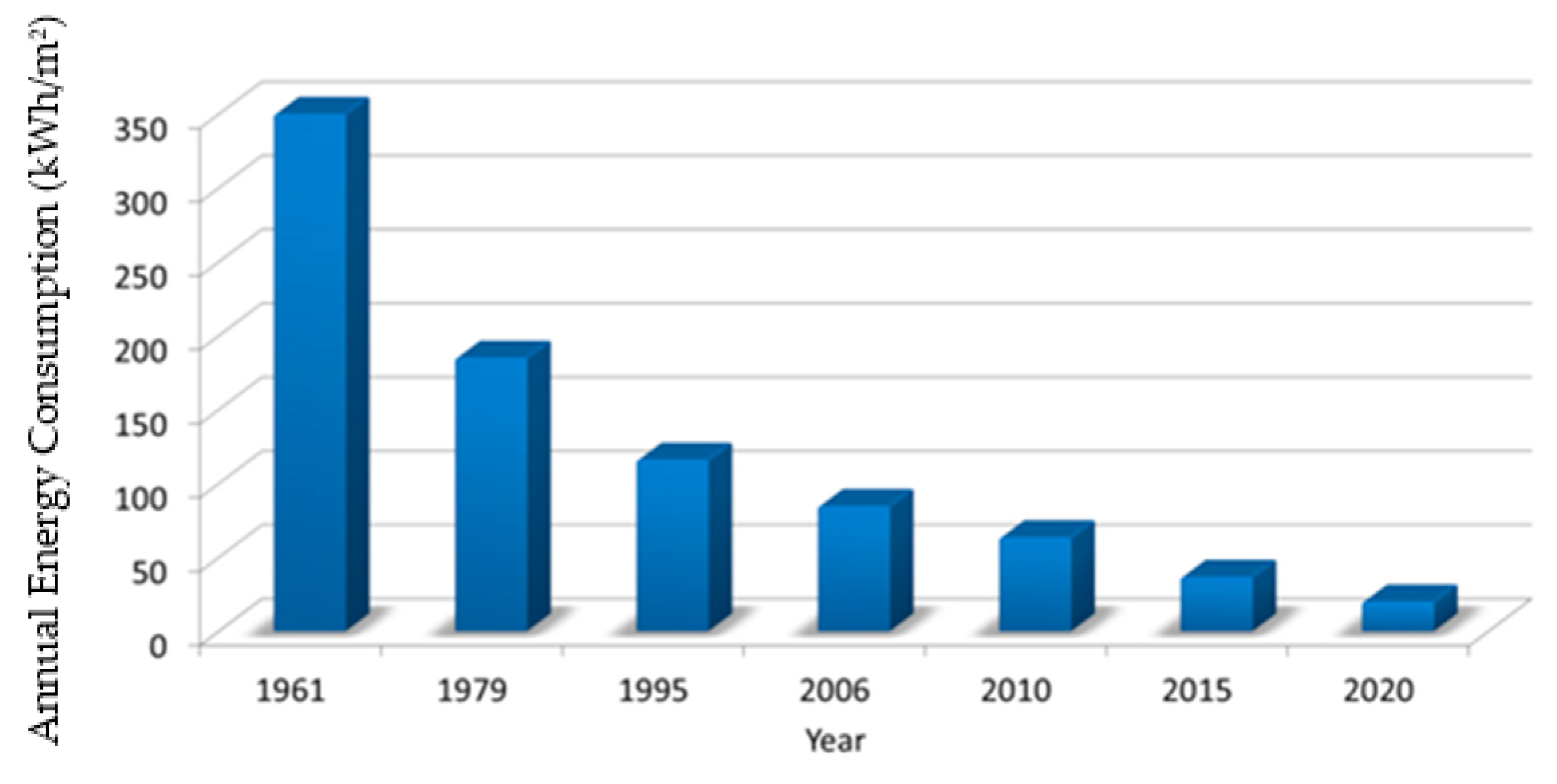
Aiming to attain a green and fossil fuel-free country, the Danish government has set very ambitious and strict energy and environmental goals by 2050 [29]. Thus, in the recent decades, a large number of energy frameworks, legislations, and plans have been highlighted in order to improve the overall energy sector efficiency. Under the new Danish plan, the potential of improving the energy performance of newly built and exiting buildings was highlighted as a major milestone to reach the objectives. In this regard, energy standards for new buildings have been dramatically tightened in the recent years in terms of building physical envelope design and energy systems operation and management [30]. Figure 2 provides an overview on the evolution of the maximum allowed yearly primary energy consumption for a 150 m² Danish residential building, as set by the successive Danish building regulations from the 60′s until now [31]. It is clear from Figure 2 that large energy savings could be attained with newly energy efficient buildings design and operation when compared to old buildings.

In addition to new buildings, efforts have targeted exiting buildings, the largest being the “Strategy for energy renovation of the existing building stock” [32]. The strategy, which was issued in 2014, comprises a list of initiatives aiming to establish the route to energy-efficient buildings in tomorrow’s Denmark through systematic and cost-effective retrofit projects throughout the country. This strategy was driven by the fact that around 80% of the Danish buildings were built before 1980 and the majority of these buildings have been retrofitted or will require retrofitting in the very near future. The ultimate aim of this energy retrofit strategy is to reduce energy consumption in existing buildings by 35% in 2050. Consequently, large retrofit projects were launched all around the country in the last decade, mainly in the big cities [33]. However, the current trend in retrofitting existing buildings is that building energy retrofit projects are driven by the need for a whole or part-modification and change in a certain aspect or specification of the building [34]. Therefore, it is led by a reactive decision-making and, thus, missing out on a cost-effective and energy efficient planning along with the absence of any systematic screening and selection process. For example, although additional insulation to the external walls and roofs of the building could lead to substantial heating and cooling energy savings, this solution is not a general best solution for all buildings of different types and systems [35].

In recent decades, a large block of theoretical investigations and practical applications in the field of building energy retrofit has been heavily presented in the literature, targeting different aspects, including energy policies, developed methodologies, business models, economic and environmental assessments, in addition to technical energy retrofit measures investigation, assessment, and demonstration [36,37]. Among these, residential sector and private houses investigations have the ultimate share with few studies targeting commercial and non- residential buildings. Rose et al. [38] has reported the energy retrofit projects of four non-residential buildings in Denmark, with two office buildings, cultural building, and a daycare center. The set of implemented measures were highlighted and the impact of carrying out the retrofit projects in the real case buildings was presented and evaluated. As a result, the authors reported an average of 65% savings on the overall energy consumption due to retrofitting the four buildings. Odgaard et al. [39] targeted old Danish buildings that were built before 1930, and the investigation concentrated on improving the building’s physical envelope and components constructions. Some of the common implemented techniques were adding around 10 cm of insulation to exterior brick walls, along with exchanging windows and adding a heat recovery unit to the ventilation systems. Savings up to 70% on the energy consumption was reported. In a recent study, Jradi et al. [35] carried out a comprehensive assessment of the trade-off between deep energy retrofit and enhancing the building systems intelligence quotient within an overall renovation process. A case study of an office building in Denmark was considered, where a detailed EnergyPlus energy model was developed and around 19 energy retrofit measures were developed and simulated. Based on the investigation results, it was reported that measures considering the implementation of energy supply systems control and management strategies could yield huge energy savings of around 47% when compared to 49% provided by conventional deep energy retrofit measures.

Although the majority of the Danish public schools were built before the 1970, very little has been reported on the retrofitting projects of such buildings. One of the few studies was presented by Morck et al. [40], who demonstrated the reduction of the annual primary energy consumption from 200 to 75 kWh/m² through a deep energy retrofit process of a public school in Ballerup, Denmark. In 2013, the Danish city of Odense has launched the ‘Energy Lean’ project aiming to enhance the energy performance of existing public schools and correspondingly reduce the CO₂ emissions by around 40% [33]. Under the research project COORDICY [41] and in collaboration with the Odense Municipality, this work reports the post-retrofit process evaluation of three public schools in Odense. A deep energy retrofit process was implemented in the three schools and it was completed by September 2018. The retrofit projects comprise a set of energy conservation and improvement measures implemented targeting both the building envelope and various energy systems. A technical evaluation of the energy retrofit process in the schools is carried out, considering one year of operation after the completion of the retrofit actual work. Onsite data from the heating and electricity meters in the schools were collected and compared with the pre-retrofit design numbers that majorly rely on static tabulated numbers for savings evaluation. In addition, an alternative approach was proposed, where detailed calibrated dynamic energy performance models, developed for the three schools in EnergyPlus, were used in order to simulate the impact of implementing the retrofit measures. The comparison results are presented and discussed.

2. Public Schools Case Study

Generally, consultants, engineers, and designers spend the majority of their efforts in the pre-retrofit implementation phase, where different suggestions, calculations, and assessments are carried out. Based on these calculations and assessments, the customer or the building owner is promised a certain projected impact of the energy retrofit project, in terms of saving energy consumption and, hence, improving the overall performance of the targeted building or facility. However, very little is being done after the retrofit project is implemented, which is the most important part of the project for the customer or the user. This post assessment phase or continuous commissioning of the retrofit project is crucial to ensure that the implemented improvement measures have yielded the positive impacts that were projected at the design phase. In this work, a case study of three public schools is considered for post-retrofit process evaluation and assessment. The three schools were heavily retrofitted by September 2018 with various improvement measures targeting buildings envelope and energy systems. Below, overall information on the three schools will be presented. The three schools’ identity is kept anonymous and, thus, will be called ‘School A’, ‘School B’, and ‘School C’.

2.1. School A

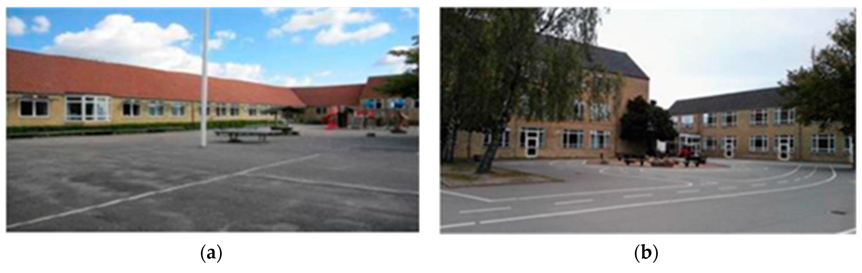
School A as shown in Figure 3a, is an elementary public school comprising 16 building blocks spanning over an area of 11,900 m². The school blocks are of different ages, where the first four blocks were built in 1954, and then additional blocks were constructed in 1967 and later in 1974. The blocks are used majorly for teaching, along with two activities blocks and a sports arena. In 2018, the school has a total number of 677 students with around 31 full time teachers. The retrofit process of School A targeted all the 16 building blocks, where the two blocks built in 1974 has exhibited only lights upgrade.

2.2. School B

School B, as shown in Figure 3b, is a primary public school with 12 building blocks across an indoor area of around 8700 m². The school was first built in 1953 with 10 blocks, and then in 1990 an extension was constructed with two blocks for teachers’ residence and lunch and meeting rooms. The majority of the blocks are used for teaching and meetings, in addition to two gym halls, party room, and storage depots. In 2018, around 536 students attended the school with 27 full time teachers. The retrofit process of School B only targeted the 10 blocks built in 1953.

2.3. School C

School C is a primary public school with 11 blocks and overall indoor area of around 8900 m². The first part of the school buildings was built in 1961, where two other blocks were added in 1971 and 1996. The majority of the buildings comprise classrooms and lecturing halls, in addition to an activity hall and a sports arena. The overall number of students attended the school in 2018 was 507 with 28 full time staff. The retrofit process of School C targeted all 11 building blocks.

2.4. Schools Characteristics

Table 1. Schools specifications and characteristics.

	School A	School B	School C
Indoor Floor Area	11,900 m2	8700 m2	8900 m2
Construction Date	1954	1953	1961
Number of Blocks	16 buildings	12 buildings	11 buildings
Number of Students	677 (2018)	536 (2018)	507 (2018)
Number of Teachers	31 (2018)	27 (2018)	28 (2018)
Operation Hours	6:30–19:00	6:30–19:00	6:30–19:00
Exterior Walls	300 mm brick/100 mm wood along with 75–150 mm mineral wool insulation. 120 mm lightweight concrete/in the teachers’ residence is equipped with 50 mm insulation. Basement walls are made of 350 mm light concrete.	Original exterior walls from 1953 are built with massive 480 mm thickness bricks with an overall U-value of 1 W/m2·K. Hollow walls at SFO are of 300 mm brick and 75 mm insulation of 0.42 W/m2·K U-value.	240–350 mm Brick with 125–150 mm insulation in 9 blocks. In the two newer building blocks, 150 mm lightweight concrete is implemented with 200–250 mm mineral wool insulation.
Roofs and Ceiling	Roof tiles, unheated roof space. In the four blocks built in 1954, the ceiling is composed of 120–170 mm brick with 75 mm mineral wool insulation. In the newer blocks, 200–250 mm brick is used with around 150–200 mm mineral wool insulation.	Roof tiles with unheated roof space. Roof is mainly 200–250 mm brick with 170 mm insulation with 0.2 W/m2·K U-value. Flat roofs have 100 mm insulation with U-value of 0.36 W/m2·K, where roof in the SFO has 200 mm insulation.	A flat roof made up of 200–250 mm brick with 50–150 mm mineral wool insulation in nine blocks. The two new blocks built in 1971 and 1996, the brick walls are equipped with 200–220 mm mineral wool insulation.
Floors	100–150 mm concrete with 50 mm lightweight expanded clay aggregate/100 mm mineral wool insulation	150 mm uninsulated concrete and 50 mm lightweight expanded clay aggregate in the basement	150 mm concrete with 50–100 mm mineral wool insulation
Windows and Doors	Mainly double-glazed windows and doors of U-value ranging between two and 3 W/m2·K, with single-glazed windows in the four blocks built in 1954	The school windows were retrofitted in the early 2000′s to double-glazed windows of U-value ranging from 2.2 to 3.1 W/m2·K with single-glazed windows and doors in two blocks built in 1953. The basement has single-glazed windows of 4.9 W/m2·K U-value.	Double-glazed windows of U-value in the region of 2.8 W/m2·K and doors with many single-glazed components in all blocks
Heating System	Direct district heating loop with multiple water circulation pumps and radiator/s in each room	Direct district heating loop with multiple water circulation pumps and radiator/s in each room	Direct district heating loop with multiple water circulation pumps and radiator/s in each room
Domestic Hot Water	Centralized production in a storage buffer tank	Centralized production using APV heat exchangers in a 400-L storage tank with 70 mm mineral wool insulation	Centralized production in two storage tanks of 300 and 1500-L storage with 100 mm mineral wool insulation
Heating Manage-ment	Central heating control with heating setpoint in each building block	Central heating control with heating setpoint in each building block	Central heating control with thermostatic valves in some blocks
Ventilation	Mainly mechanical ventilation systems (ranges between 1200 and 10,000 m3/h nominal air flow) with natural ventilation in one block and heat recovery units	A mix between mechanical ventilation systems and natural ventilation in the majority of blocks with heat recovery units	All blocks have mechanical ventilation systems (ranges between 700 and 6000 m3/h nominal air flow in different blocks) with heat recovery units
Lighting	A mix of T5 and T8 light tubes with motion sensors in specific zones	A mix of one and three lines T5 light tubes with motion sensors in some classrooms	A mix of T5 and T8 light tubes with motion sensors in bathrooms, and technical rooms

summarizes the detailed characteristics and specifications of each of the three considered public schools. This includes information on the schools’ use, physical envelope constructions, energy systems design, operation, and management.

3. Deep Energy Retrofit Projects

As noted in Section 2, the three schools considered were constructed within the period (1950–1960), and the presented characteristics along with the reported energy consumption shows that major energy retrofits are needed to enhance the energy performance. Thus, the three schools were among the prioritized public schools in Odense to be considered under the Energy Lean retrofit project [33]. Based on detailed assessment of the current status, design information, energy labels, field visits, technical meetings, interviews, and feedback from the users, a list of energy retrofit measures were suggested by the engineering consultants in order to improve the schools’ performance. The deep energy retrofit projects in the three schools were carried out and completed by September 2018.

Table 2. Deep energy retrofit improvement measures implemented in each of the three schools.

School A	School B	School C
Upgrading the lights in all the building blocks with energy efficient T5 and T8 tube LED lights. Insulating the interior layer of the attic space area of 7400 m2 under the tilted roof in nine building blocks with 250 mm mineral wool. Insulating an area of 95 m2 of exterior walls in one block with 190 mm of mineral wool insulation on the interior side. Upgrading single-glazed windows, glass doors in 7 blocks with double-glazed energy efficient components (design U-value of 1.3 W/m2·K) with new frames. Upgrading skylights in 8 building blocks with energy efficient glazing of U-value around 1.4 W/m2·K. Replacing four domestic hot water circulation pumps. Upgrading the strategy for heating setpoint management in each of the building blocks. Insulating pipes, valves and pumps in all technical rooms.	Upgrading the lights in 10 out of the 12 building blocks with energy efficient T5 tube LED lights. Insulating the interior layer of the attic space area of 150 m2 under the tilted roof with 200 mm mineral wool. Insulating 120 m2 of exterior walls with 150–200 mm of mineral wool on the interior side. Upgrading single-glazed windows and glass doors in 4 blocks to energy efficient thermal double-glazed components (U-value around 1.4 W/m2·K) with upgraded frames. Replacing three domestic hot water circulation pumps. Proposing heating system setpoint management framework in each of the blocks. Installing motion sensors in some classrooms. Insulating pipes, valves and pumps in all technical rooms.	Upgrading the lights in all the building blocks with energy efficient T5 and T8 tube LED lights. Insulating flat roof of four blocks of around 1800 m2 area with 150–300 mm batt insulation on the interior layer. Insulating an interior side of the exterior wall area of 850 m2 with 100 mm mineral wool. Upgrading single-glazed windows, glass doors and some skylights in 6 blocks with double-glazed energy efficient components (design U-value of 1.3 W/m2·K) along with new frames. Replacing two domestic hot water circulation pumps. Proposing heating system setpoint management framework in some of the blocks. Insulating pipes, valves and pumps in all technical rooms.

presents an overview on the selected and implemented energy improvement measures and modifications in each of the three schools.

4. Post-Retrofit vs. Pre-Retrofit Performance

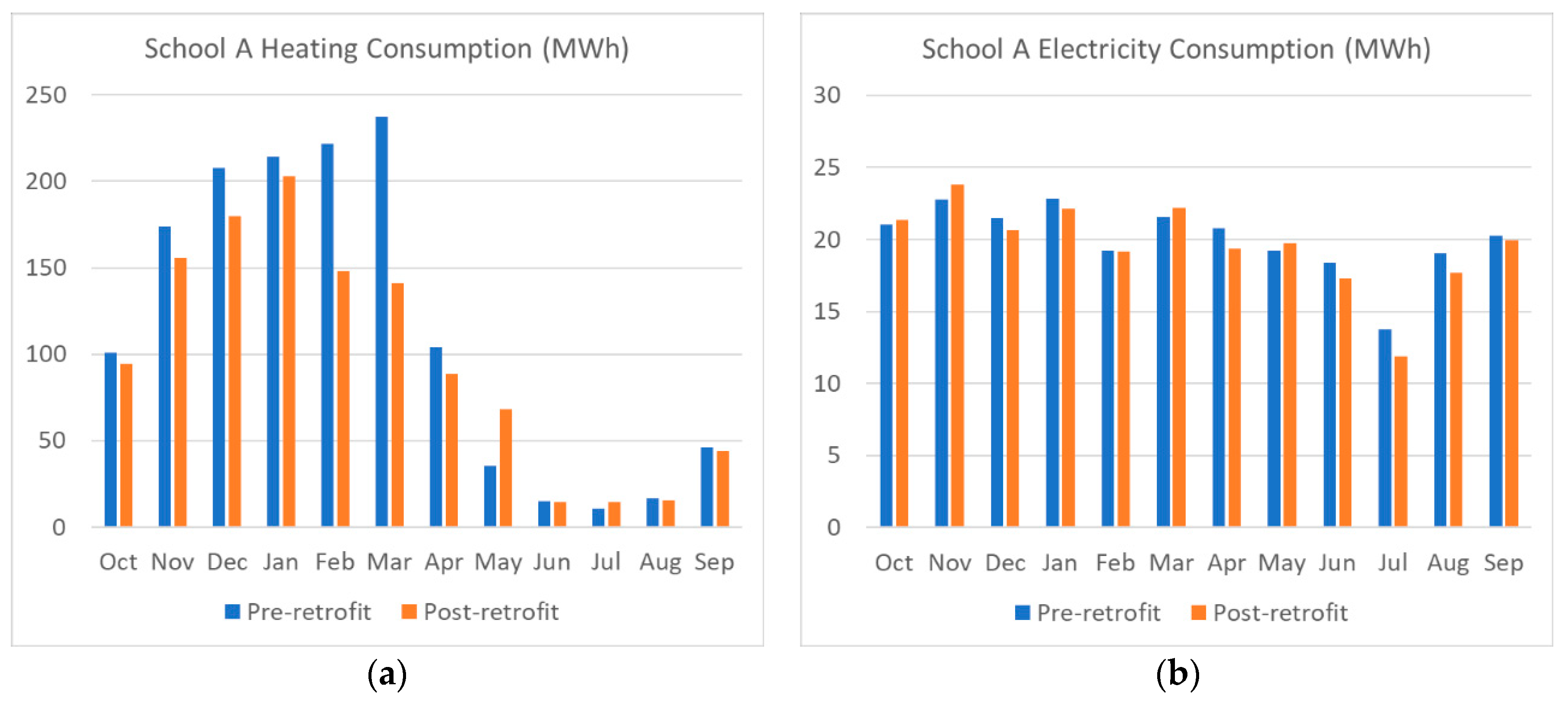
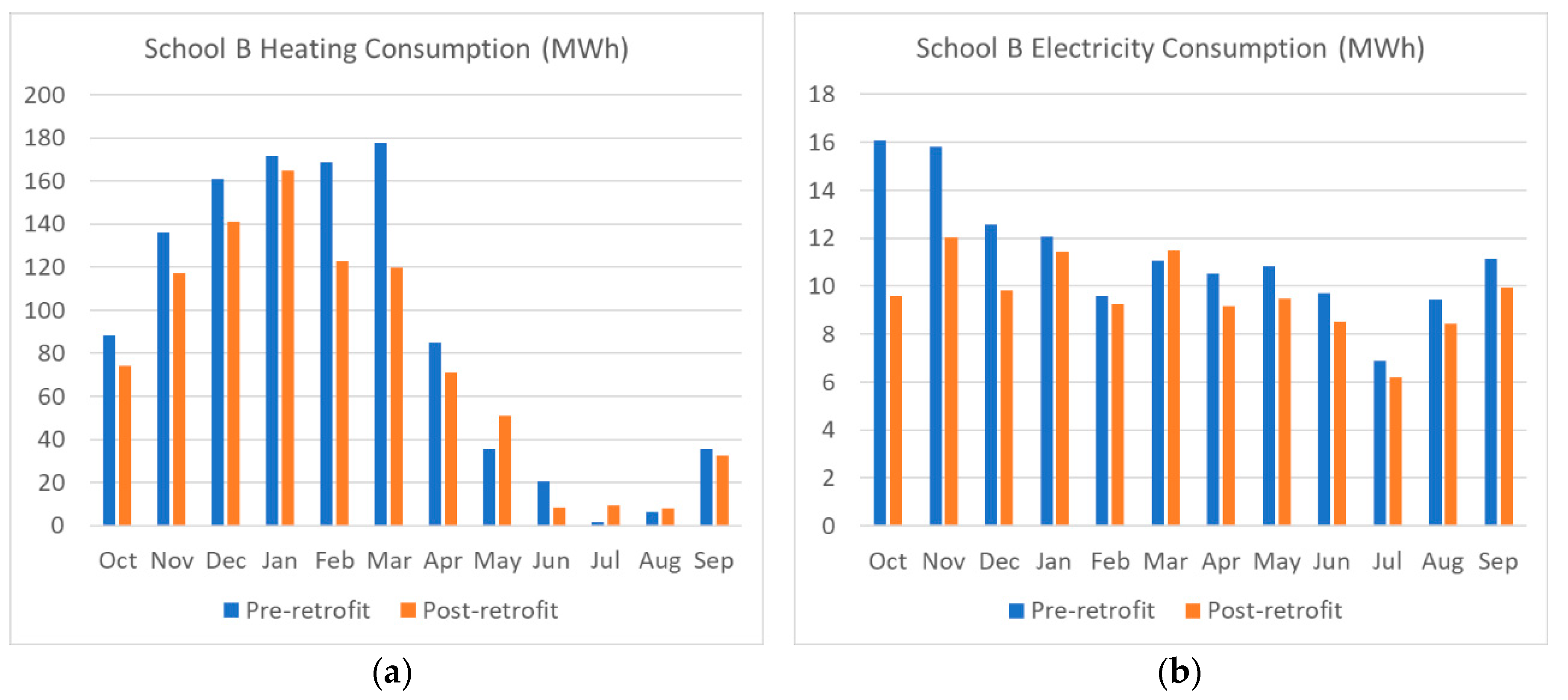
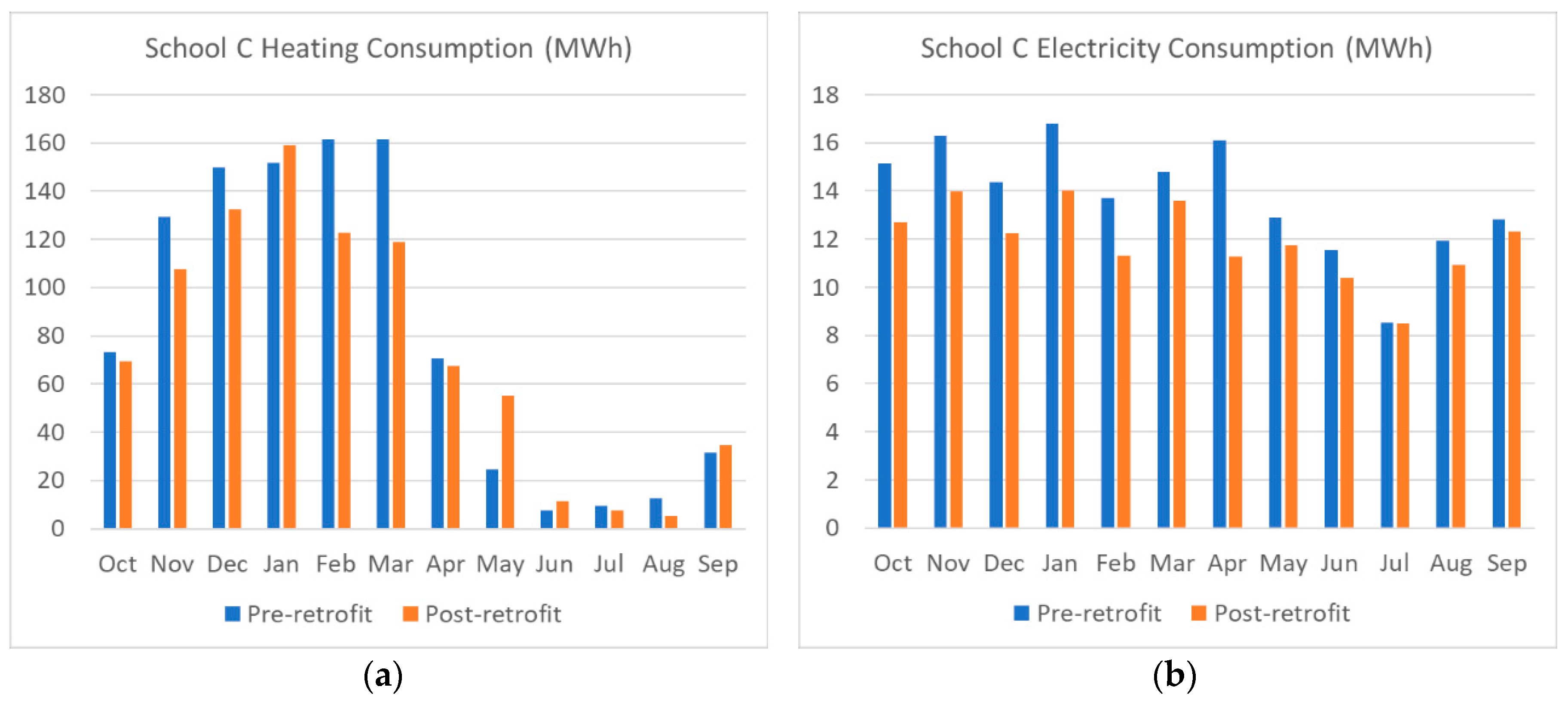
An overall post-evaluation of the energy retrofit projects that were carried out in the three public schools is presented. The technical impacts of implementing the retrofit projects will be evaluated, considering a one-year period of the schools’ operation after the completion of the retrofits. Onsite monitored data is reported on a holistic level, mainly the schools’ overall heating and electricity consumption. Therefore, overall district heating energy consumption data from heating meters are collected on the level of the whole school, while the overall school electricity consumption meter is also considered in the analysis. The energy performance monitoring post-retrofit period chosen in this investigation is a year spanning from October 2018 to September 2019. The energy consumption of the schools in this period will be compared with the energy consumption in the pre-retrofit period from October 2017 to September 2018. Figure 4, Figure 5 and Figure 6 shows the monthly heating and electricity consumption of the three schools, when comparing the pre-retrofit data with the post-retrofit data.

Overall, the impact of implementing the energy retrofit projects is very different in the three schools, majorly regarding the effect on the heating and electricity consumption. While the data report an overall reduction in the electricity consumption for the majority of the months in the three schools, the case is different in terms of heating consumption. For example, the heating energy savings for the three schools range from 23% to 33% in February, and around 26% to 40% in March. Nevertheless, some months still exhibit higher energy consumption for the post-retrofit period when compared to the pre-retrofit period, as noted for the month of May.

Table 3. Summary of the retrofit projects impact in the three schools considered.

	School A	School B	School C
Pre-retrofit annual heating consumption (MWh)	1383	1088	983
Post-retrofit annual heating consumption (MWh)	1167	920	892
Annual Heating Savings (%)	15.7	15.4	9.3
Pre-retrofit annual electricity consumption (MWh)	240	136	165
Post-retrofit annual electricity consumption (MWh)	235	115	143
Annual Electricity Savings (%)	2.2	15.0	13.2

summarizes the overall technical impacts of the three retrofit projects based on the actual data collected. It is reported that the three schools exhibit a reduction on the heating and electricity consumption profiles after one year of the retrofit project implementation. While Schools A and B have an overall annual heating savings of around 15%, School C registers only 9% reduction on the heating demand. On the other hand, School B exhibits the largest electricity savings of around 15%, when compared to 13% for School C and just over 2% for School A.

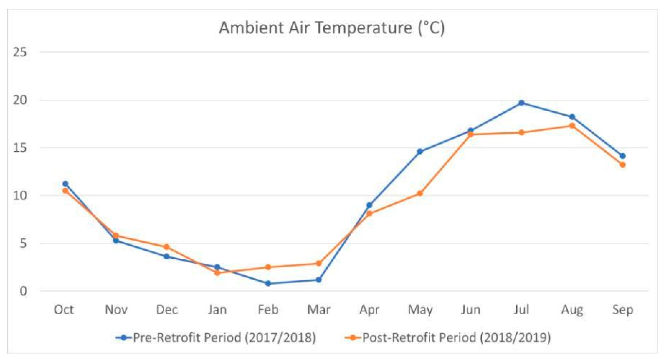
While the building electricity and heating consumption are mainly governed by the systems and devices efficiency and operation, as well as the usage and management of the building, the heating consumption is largely affected by the ambient air temperature profile. Thus, the actual monthly average air temperatures recorded in Odense for the pre-retrofit and post-retrofit periods are shown in Figure 7. It could be noted that there is not that much difference between the two profiles, where the ambient air temperature is comparable or even lower in the majority of the months. The two major exceptions are the months of February and March. Specifically, February and March (2019) in the post-retrofit year are warmer than February and March (2018) months in the pre-retrofit year considered. This also supports the fact that a very large heating energy consumption reduction is exhibited after retrofitting in those two months (23–40%). It means that part of the energy savings in these months is due to the warmer weather and not only due to the energy retrofit improvements. On the other hand, the maximum difference in terms of the overall yearly temperature is depicted in May, where the ambient air temperature in May 2019 after retrofit is, on average, lower than the temperatures that were recorded in May 2018 before the retrofit process with around 5 °C. This is also reflected by the number that is shown in Figure 6, where the schools consume almost double the amount of heating in May after retrofit when compared to the consumption before retrofitting.

5. Retrofit Design Estimations vs. Dynamic Energy Simulations

5.1. Static Estimations vs. Dynamic Simulations

In terms of the energy retrofitting work, the extent and the number of measures implemented in each building block in the three schools vary considerably. While some school blocks have only been targeted by implementing new LED lights, others have undergone an extensive retrofit process with walls and roofs insulation and windows exchange. In addition, and due to the absence of energy data on the level of single building blocks, the decision was to implement the overall modeling and simulation process on the level of all the school blocks and compare the whole school energy performance before and after retrofitting, rather than comparing on the level of the single blocks.

A comparison will be presented between the real data that were collected from the heating and electricity meters in the schools with the pre-retrofit design numbers that majorly rely on static tabulated numbers for savings evaluation. In addition, an alternative approach is proposed, employing calibrated dynamic energy models developed for the schools in EnergyPlus, in order to simulate the impact of implementing the retrofit measures. Thus, it is important to define two notions, as follows:

-

Static Design Estimations: these are the calculations and estimations that were performed by the consultant or engineer in the pre-retrofit design stage to evaluate the expected impact of the retrofit improvements. Generally, these estimations use tabulated data using pre-defined factors and assumptions in order to estimate the technical impact [42,43,44]. One example of the tools using tabulated static data and assumptions to evaluate building performance is BE18 [45], the official tool for building performance technical assessment and certification in Denmark. While the tool is very effective in assessing whether the building complies with the building standards regarding building envelope and energy consumption, it fails to capture the impact of dynamic changes and boundary conditions on the building performance. In addition, it imposes a large number of assumptions and uncertainties, including the assumption that the whole building is made up of one big room, static occupancy numbers, constant ambient air temperatures, and fixed energy systems parameters.

-

Dynamic Model Simulations: These are the predictions of a dynamic building energy model (in this study developed in EnergyPlus) reporting the results of the retrofit measures technical impacts. In this approach, different building specifications and characteristics are considered, as well as occupants’ usage of the building and dynamic weather conditions.

5.2. Building Energy Modeling and Simulation Methodology

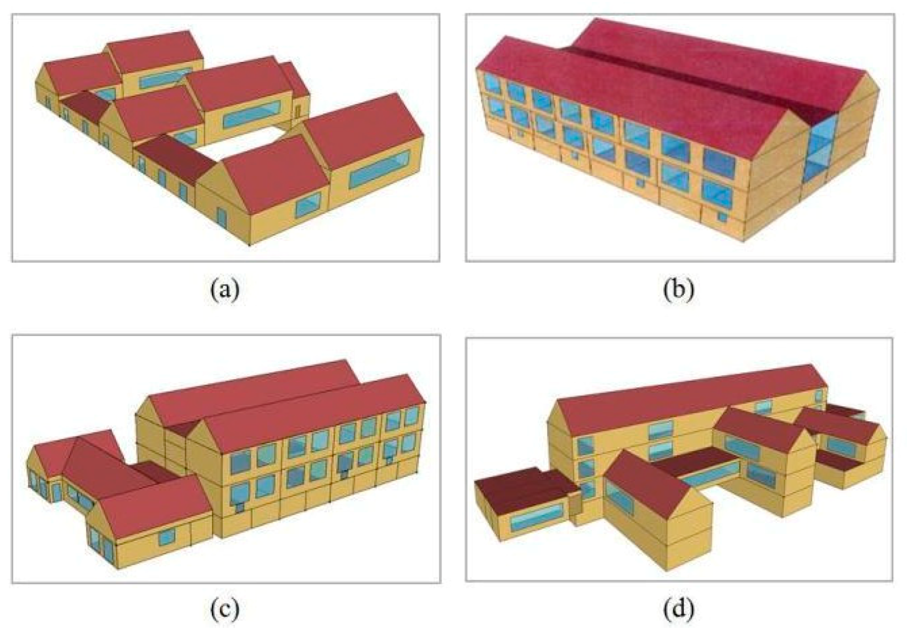
The overall holistic building energy modelling and simulation methodology that were developed by Jradi et al. [46] were employed to model and simulate the schools’ energy performance. Three tools were used, Sketchup Pro for developing the detailed 3D architectural model of the school, OpenStudio to develop the energy model and define various building specifications and characteristics, and finally the EnergyPlus engine for running an annual energy performance simulation for the three schools.

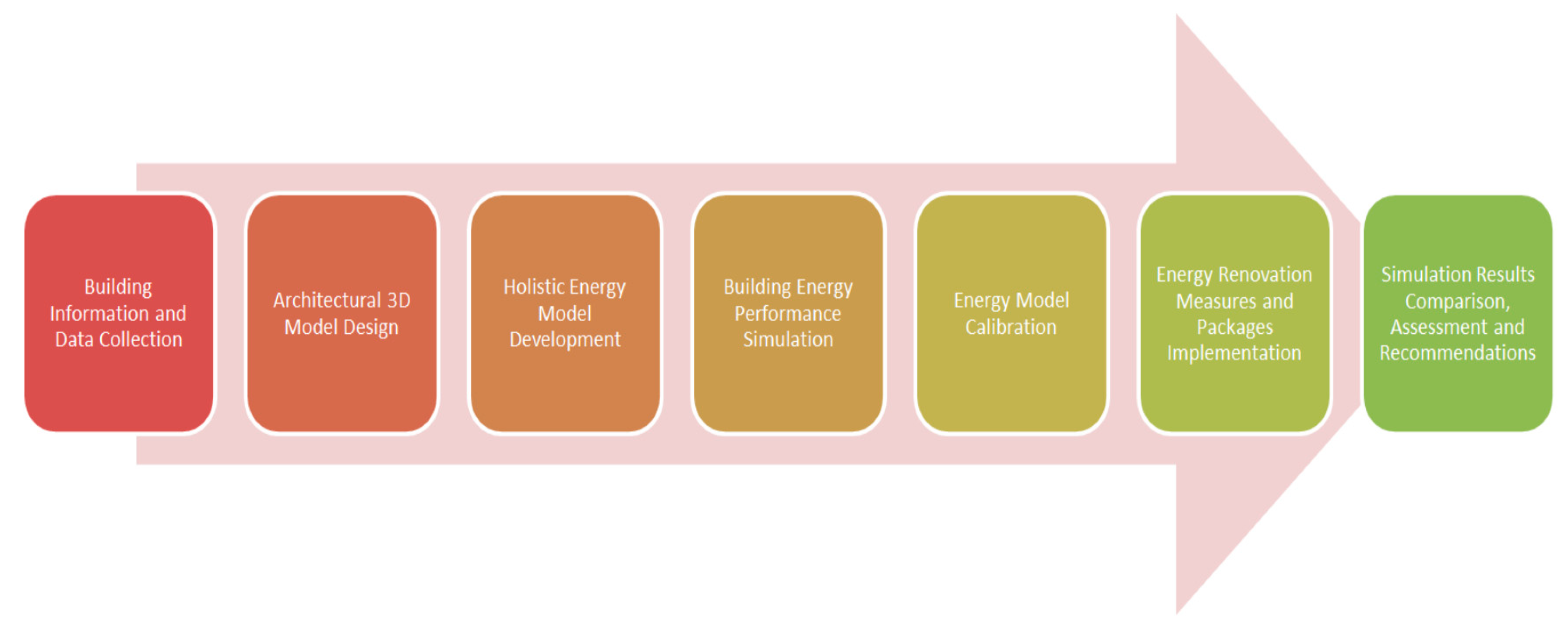
A comprehensive and detailed energy model is needed in order to carry out a holistic and accurate simulation of building energy performance. Such a model shall take into account various building specifications along with boundary conditions, operational dynamics, and ambient environment. Thus, inputs to a proper and detailed dynamic energy model include, but are not limited to, location and orientation, building envelope properties, construction materials, HVAC systems, climatic conditions, building services, equipment and lights, room types and schedules, occupancy behavior, and patterns. In this study, the EnergyPlus simulation engine is used to carry out a detailed dynamic annual building energy performance prediction. EnergyPlus is very well validated in the field of building energy modelling with various capabilities in terms of building operation simulation and performance prediction. In addition, two supporting tools are employed in order to allow for a smooth transition from building 3D architectural model to a full-scale building energy model. Google Sketchup Pro is first employed to create the 3D model of the considered schools with an accurate depiction of the different blocks geometry and orientation including the detailed rooms, spaces and thermal zones allocation. The 3D model is then introduced to OpenStudio, which allows for a more user-friendly interface for building energy model development compared to the default EnergyPlus tool. In OpenStudio, all of the building characteristics and various specifications mentioned above are defined and highlighted including different building design and operational parameters. Figure 8 provides an overall picture of the modelling and simulation process that are adopted in this work.

The overall modeling and simulation methodology employed for the three schools starts with the (1) Building Information and data collection phase, where all school building blocks information and design and operational parameters are collected, along with geometry drawings, datasheets, systems information, and construction sets. Subsequently, in the (2) Architectural 3D model design phase, a full 3D model of the building is drawn in Sketchup Pro with all blocks’ details and geometry. This 3D model is then introduced to OpenStudio in (3) Holistic energy model development, in order to define all specifications and develop the holistic schools’ energy models. When the schools’ models are ready, a complete energy performance simulation is carried out in (4) Building energy performance simulation. This is followed by a (5) Energy model calibration phase, where energy data that were collected from meters in the schools are used to calibrate the developed dynamic energy model. As the calibrated dynamic model of the school is ready, phase (6) Energy renovation measures and packages implementation is performed, where a large number of retrofit measures and packages listed above in each school is implemented in the energy model in order to simulate the impact of retrofitting the various building blocks. Finally, the simulation results are obtained in the final phase (7) Simulation results comparison, assessment, and recommendations, where the results of the school retrofit project impacts are reported and compared to the pre-retrofit data to draw up conclusions and recommendations.

Figure 9 shows the Sketchup models for four blocks of School B. Similarly, all the three schools’ blocks are modelled to an acceptable level of details, using design specifications, collected information, technical drawings, filed visits, and inspections. After model development in OpenStudio, the three schools’ holistic models were calibrated using actual energy consumption data for heating and electricity consumption collected onsite with the aid of the OpenStudio Parametric Analysis Tool [47]. The main parameters selected for calibration include infiltration rates, fans pressure rise, pump and equipment efficiencies, along with load capacity and operation schedules. The maximum reported uncertainty of the calibrated model compared to actual data for the three schools is 1.4% and 2.1% for monthly electricity and heating consumption, respectively [48]. Subsequently, for each school, the calibrated model is used to implement and simulate all of the energy improvement and retrofit measures agreed on and listed in Table 2.

5.3. Comparison and Assessment

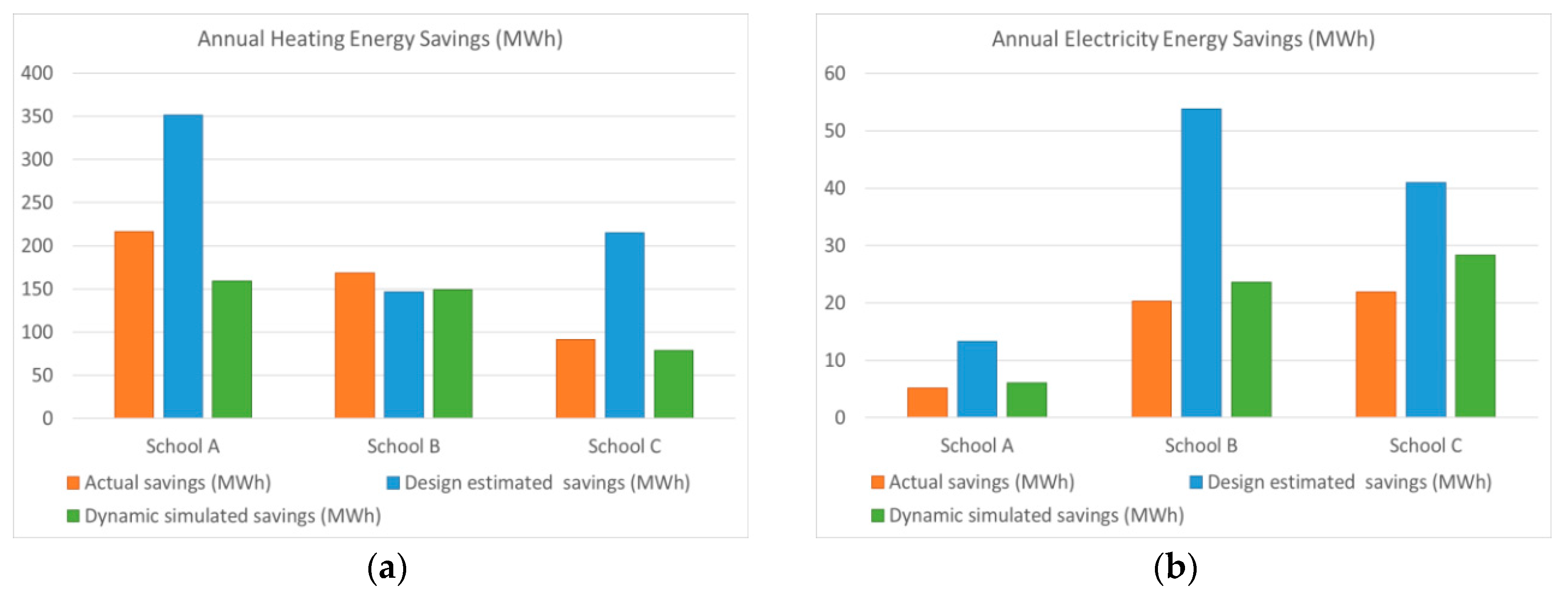
When considering the results of the dynamic energy simulations for the three retrofitted schools, an overall comparison is performed between design estimated, dynamic simulated. and actual reported heating and electricity energy savings for the three investigated schools, as shown in Figure 10. It could be noted that both static design estimations and dynamic energy simulations overestimate the electricity savings in the three public schools due to the retrofit projects. However, it is shown that the dynamic simulations more accurately predict the technical impact of the retrofit improvements in the three schools in terms of electricity consumption savings, where design estimations are largely off with a big margin. In terms of heating consumption, the dynamic energy simulations for the three schools underestimate the annual heating energy savings in the three schools with an acceptable margin of error. On the other hand, static design estimations are again overestimating the heating energy savings with a large deviation when compared to actual reported data in Schools A and C, where the estimations for School B are much more accurate with acceptable error margin.

Table 4. Energy savings relative error for design estimations and dynamic simulations compared to actual collected data in the three schools.

	School A	School B	School C
Design estimated heating savings relative error (%)	−62.1	13.0	−135.3
Dynamic simulated heating savings relative error (%)	26.5	11.3	14.1
Design estimated electricity savings elative error (%)	−155.7	−165.0	−87.2
Dynamic simulated electricity savings relative error (%)	−17.3	−16.2	−29.2

provides a more detailed assessment on the relative error in terms of annual heating and electricity savings, as estimated by static design numbers from one side and the dynamic energy simulations on the other side, when compared to the actual monitored numbers from the three schools. Based on the reported data, it is clear that the dynamic energy model simulations predict in a fairly higher accuracy, compared to the static estimations, the technical impact of the retrofit projects in the three schools. The respective performance gap between the actual real energy savings and simulated numbers in the three schools is in the range of 11–26% and 16–29% for heating and electricity consumption. On the other hand, the static design estimations are very far from being accurate in estimating the impact of the retrofit projects and the energy savings in the three schools, except for the heating energy savings in School B with a relative error of around 13%. Overall, it is found that dynamic energy simulations using a detailed and calibrated holistic energy model could provide a very good prediction on the impact of a retrofit project with an acceptable performance gap and much higher accuracy when compared to conventional approaches while using tabulated assumptions and static design estimations.

6. Conclusions

The current trend in the majority of Danish energy retrofit applications and projects is that the retrofit process is driven by a reactive decision making, which is always accompanied by the lack of a cost-effective and energy efficient planning and the absence of a systematic screening and selection among improvement measures. The largest share of efforts put in any retrofit project is at the pre-retrofit design and implementation stages, where calculations, assessment, and evaluations of the retrofit options are carried out. On the other hand, what matters for any owner or building user in a retrofit project is to have a building of improved performance and to attain the savings promised at the design stage. However, there is an overall lack of commissioning of retrofitted building performance at the post-retrofit stage to assess the building performance after being retrofitted and to ensure that the savings are attained.

In this work, three public schools were considered for post-retrofit evaluation. The schools have undergone a deep energy retrofit process by September 2018, with multiple energy conservation and improvement measures implemented targeting the building envelope and different energy systems. After the completion of the retrofit projects, the three schools’ energy performance was monitored for a year on the holistic level, mainly electricity and heating consumption profiles. When considering the data collected, an overall evaluation of the retrofit projects was carried out to assess the technical impacts. It was shown that the respective energy savings in the three schools are within the following ranges (9 to 16%) for heating and (2 to 15%) for electricity consumption. In addition, a comparison was performed between the attained energy savings and the promised ones at the retrofit design stage. The average performance gap between the expected and real numbers for the three schools was around 61% and 136% for annual heating and electricity savings, respectively. On the other hand, an alternative approach was proposed and evaluated. In this regard, a calibrated dynamic energy performance model for each school was developed in EnergyPlus and employed in order to simulate the technical impacts of implementing the retrofit measures. The results of comparing the dynamic simulations with the actual data were much more satisfactory, as compared to the case of the design numbers. The performance gap between the real and simulated savings in the three schools was in the range of 16–29% for electricity and 11–26% for heating consumption.

Based on the results of this post-retrofit evaluation study in the schools, it is concluded that the dynamic model simulations of the retrofit processes allow for reducing the performance gap between the expected and the actual energy savings, when compared to tabulated static approaches, which was found to be inaccurate with a large margin of error. This study highlights the added value of using the alternative dynamic modelling and simulation approach in predicting the expected impacts of retrofit projects, as compared to the static design numbers. This demonstrates the need for holistic and comprehensive tools for buildings energy retrofit design and assessment, being simple to use and accurate at the same time. This will aid the retrofitting decision-making and enhance the building users’ and owners’ trust and satisfaction.

References

- Jradi, M.; Gamboa, A.Z.; Veje, C. Simulation and parametric analysis of an office building energy performance under Danish conditions. In Proceedings of the 14th International Conference on Sustainable Energy Technologies (SET 2015), Nottingham, UK, 25–27 August 2015. [Google Scholar]
- Dean, B.; Dulac, J.; Petrichenko, K.; Graham, P. Towards Zero-Emission Efficient and Resilient Buildings: Global Status Report; International Energy Agency (IEA) for the Global Alliance for Buildings and Construction: Paris, France, 2017. [Google Scholar]
- Anand, C.K.; Amor, B. Recent developments, future challenges and new research directions in LCA of buildings: A critical review. Renew. Sustain. Energy Rev. 2017, 67, 408–416. [Google Scholar] [CrossRef]
- European Commission. Directive 2010/31/EU of the European Parliament on the Energy Performance of Buildings; European Union: Brussels, Belgium, 2010. [Google Scholar]
- European Commission. Directive 2018/844 of the European Parliament and of the Council of 30 May 2018 Amending Directive 2010/31/EU on the Energy Performance of Buildings and Directive 2012/27/EU on Energy Efficiency; European Comission: Brussels, Belgium, 2018. [Google Scholar]
- Frei, B.; Sagerschnig, C.; Gyalistras, D. Performance gaps in Swiss buildings: An analysis of conflicting objectives and mitigation strategies. Energy Procedia 2017, 122, 421–426. [Google Scholar] [CrossRef]
- Zou, P.X.W.; Wagle, D.; Alam, M. Strategies for minimizing building energy performance gaps between the design intend and the reality. Energy Build. 2019, 191, 31–41. [Google Scholar] [CrossRef]
- Sun, C.; Zhang, R.; Sharples, S.; Han, Y.; Zhang, H. Thermal comfort, occupant control behaviour and performance gap—A study of office buildings in north-east China using data mining. Build. Environ. 2019, 149, 305–321. [Google Scholar] [CrossRef]
- Kampelis, N.; Gobakis, K.; Vagias, V.; Kolokotsa, D.; Standardi, L.; Isidori, D.; Cristalli, C.; Montagnino, F.; Paredes, F.; Muratore, P.; et al. Evaluation of the performance gap in industrial, residential & tertiary near-Zero energy buildings. Energy Build. 2017, 148, 58–73. [Google Scholar] [CrossRef] [Green Version]
- Herrando, M.; Cambra, D.; Navarro, M.; De La Cruz, L.; Millán, G.; Zabalza, I. Energy Performance Certification of Faculty Buildings in Spain: The gap between estimated and real energy consumption. Energy Convers. Manag. 2016, 125, 141–153. [Google Scholar] [CrossRef] [Green Version]
- Jradi, M.; Arendt, K.; Sangogboye, F.C.; Mattera, C.G.; Markoska, E.; Kjærgaard, M.B.; Veje, C.; Jørgensen, B.N. ObepME: An online building energy performance monitoring and evaluation tool to reduce energy performance gaps. Energy Build. 2018, 166, 196–209. [Google Scholar] [CrossRef] [Green Version]
- Zou, P.X.; Xu, X.; Sanjayan, J.; Wang, J. Review of 10 years research on building energy performance gap: Life-cycle and stakeholder perspectives. Energy Build. 2018, 178, 165–181. [Google Scholar] [CrossRef]
- Robinson, J.F.; Foxon, T.J.; Taylor, C.G. Performance gap analysis case study of a non-domestic building. Proc. Inst. Civ. Eng. Eng. Sustain. 2016, 169, 31–38. [Google Scholar] [CrossRef] [Green Version]
- Jankovic, L. A method for reducing simulation performance gap using Fourier filtering. In Proceedings of the Building Simulation 2013: 13th Conference of International Building Performance Simulation Association, Chambery, France, 26–28 August 2013. [Google Scholar]
- Imam, S.; Coley, D.A.; Walker, I. The building performance gap: Are modellers literate? Build. Serv. Eng. Res. Technol. 2017, 38, 351–375. [Google Scholar] [CrossRef] [Green Version]
- Markoska, E.; Jradi, M.; Jørgensen, B.N. Continuous commissioning of buildings: A case study of a campus building in Denmark. In Proceedings of the 9th IEEE International Conference on Cyber, Physical, and Social Computing (CPSCom 2016), Chengdu, China, 16–19 December 2016. [Google Scholar]
- Gaetani, I.; Hoes, P.-J.; Hensen, J.L. Occupant behavior in building energy simulation: Towards a fit-for-purpose modeling strategy. Energy Build. 2016, 121, 188–204. [Google Scholar] [CrossRef]
- Van Dronkelaar, C.; Dowson, M.; Burman, E.; Spataru, C.; Mumovic, D. A Review of the Energy Performance Gap and Its Underlying Causes in Non-Domestic Buildings. Front. Mech. Eng. 2016, 2, 17. [Google Scholar] [CrossRef] [Green Version]
- Hobart, C.; Thomson, D.; Dainty, A.; Fernie, S.; Drewniak, D. Closing the energy performance gap in zero carbon homes - pro-active identification, prioritisation and mitigation of causes using FMEA. In Proceedings of the 31st Annual ARCOM Conference, Lincoln, UK, 7–9 September 2015; pp. 307–316. [Google Scholar]
- De Wilde, P. The gap between predicted and measured energy performance of buildings: A framework for investigation. Autom. Constr. 2014, 41, 40–49. [Google Scholar] [CrossRef]
- Lehmann, U.; Khoury, J.; Patel, M.K. Actual energy performance of student housing: Case study, benchmarking and performance gap analysis. Energy Procedia 2017, 122, 163–168. [Google Scholar] [CrossRef]
- Petersen, S.; Hviid, C.A. The European energy performance of buildings directive: Comparison of calculated and actual energy use in a Danish office building. In Proceedings of the IBPSA-England First Building Simulation and Optimisation Conference (BSO 2012), Loughborough, UK, 10–11 September 2012. [Google Scholar]
- Figueiredo, A.; Kämpf, J.; Vicente, R.; Oliveira, R.; Silva, T. Comparison between monitored and simulated data using evolutionary algorithms: Reducing the performance gap in dynamic building simulation. J. Build. Eng. 2018, 17, 96–106. [Google Scholar] [CrossRef]
- Kim, S.H.; Augenbroe, G. Uncertainty in developing supervisory demand-side controls in buildings: A framework and guidance. Autom. Constr. 2013, 35, 28–43. [Google Scholar] [CrossRef]
- Habibi, S. The promise of BIM for improving building performance. Energy Build. 2017, 153, 525–548. [Google Scholar] [CrossRef]
- Oduyemi, O.; Okoroh, M. Building performance modelling for sustainable building design. Int. J. Sustain. Built Environ. 2016, 5, 461–469. [Google Scholar] [CrossRef] [Green Version]
- Attia, S.; Hensen, J.L.M.; Beltrán, L.; De Herde, A. Selection criteria for building performance simulation tools: Contrasting architects’ and engineers’ needs. J. Build. Perform. Simul. 2012, 5, 155–169. [Google Scholar] [CrossRef] [Green Version]
- Foldager, H.E.; Jeppesen, R.C.; Jradi, M. DanRETRO: A Decision-Making Tool for Energy Retrofit Design and Assessment of Danish Buildings. Sustainability 2019, 11, 3794. [Google Scholar] [CrossRef] [Green Version]
- Lund, H.; Mathiesen, B.V. Energy system analysis of 100% renewable energy systems—The case of Denmark in years 2030 and 2050. Energy 2009, 34, 524–531. [Google Scholar] [CrossRef]
- Building Regulation BR 18, Bygningsreglementet. Available online: http://bygningsreglementet.dk/ (accessed on 28 September 2020).
- Energy Policy Toolkit on Energy Efficiency in New Buildings—Experiences from Denmark, The Danish Energy Agency. Available online: https://ens.dk/sites/ens.dk/files/Globalcooperation/tool_ee_byg_web.pdf (accessed on 16 September 2020).
- Strategy for Energy Renovation of Buildings, Danish Ministry of Climate, Energy and Building. Available online: https://ec.europa.eu/energy/sites/ener/files/documents/2014_article4_en_denmark.pdf (accessed on 21 September 2020).
- Odense Energy Lean. Available online: https://www.odense.dk/om-kommunen/forvaltninger/by-og-kulturforvaltningen/drift-og-anlaeg/ejendom/4-gode-grunde (accessed on 5 September 2020).
- Jafari, A.; Valentin, V. An optimization framework for building energy retrofits decision-making. Build. Environ. 2017, 115, 118–129. [Google Scholar] [CrossRef]
- Jradi, M.; Veje, C.; Jørgensen, B.N. Deep Energy Retrofit vs Improving Building Intelligence: Danish Case Study. In Proceedings of the 2018 Building Performance Modeling Conference and SimBuild Co-Organized by ASHRAE and IBPSA-USA, ASHRAE, Chicago, IL, USA, 26–28 September 2018; pp. 470–477. [Google Scholar]
- Mortensen, A.; Heiselberg, P.; Knudstrup, M. Economy Controls Energy Retrofits of Danish Single-Family Houses: Comfort, Indoor Environment and Architecture Increase the Budget. Energy Build. 2014, 72, 465–475. [Google Scholar]
- Bjørneboe, M.; Svendsen, S.; Heller, A. Initiatives for the energy renovation of single-family houses in Denmark evaluated on the basis of barriers and motivators. Energy Build. 2018, 167, 347–358. [Google Scholar] [CrossRef]
- Rose, J.; Thomsen, K.E. Energy Saving Potential in Retrofitting of Non-residential Buildings in Denmark. Energy Procedia 2015, 78, 1009–1014. [Google Scholar] [CrossRef] [Green Version]
- Odgaard, T.; Bjarløv, S.P.; Rode, C.; Vesterløkke, M. Building Renovation with Interior Insulation on Solid Masonry Walls in Denmark—A study of the Building Segment and Possible Solutions. Energy Procedia 2015, 78, 830–835. [Google Scholar]
- Morck, O.; Thomsen, K.E.; Jorgensen, B.E. School of the Future: Deep Energy Renovation of the Hedegaards School in Denmark. Energy Procedia 2015, 78, 3324–3329. [Google Scholar] [CrossRef] [Green Version]
- COORDICY. Available online: http://www.sdu.dk/en/om_sdu/institutter_centre/centreforenergyinformatics/research+projects/coordicy (accessed on 29 September 2020).
- Wang, D.; Pang, X.; Wang, W.; Qi, Z.; Ji, Y.; Yin, R. Evaluation of the dynamic energy performance gap of green buildings: Case studies in China. Build. Simul. 2020, 13, 1191–1204. [Google Scholar] [CrossRef]
- Maile, T.; Fischer, M.; Bazjanac, V. Building energy performance simulation tools—A life-cycle and interoperable perspective. CIFE Work. Pap. 2007, 107, 1–49. [Google Scholar]
- Tronchin, L.; Fabbri, K. Energy performance building evaluation in Mediterranean countries: Comparison between software simulations and operating rating simulation. Energy Build. 2008, 40, 1176–1187. [Google Scholar] [CrossRef]
- BE18 Building Energy Performance Assessment Tool. Available online: https://sbi.dk/beregningsprogrammet/Pages/Start.aspx (accessed on 30 October 2020).
- Jradi, M.; Veje, C.; Jørgensen, B. Deep energy renovation of the Mærsk office building in Denmark using a holistic design approach. Energy Build. 2017, 151, 306–319. [Google Scholar] [CrossRef]
- OpenStudio Parametric Analysis Tool. 2019. Available online: http://nrel.github.io/OpenStudio-user-documentation/reference/parametric_studies (accessed on 26 August 2020).
- Jradi, M.; Veje, C.; Jørgensen, B.N. Technical and Economic Assessment of a Danish Public School Energy Renovation using Dynamic Energy Performance Model. In Proceedings of the 2018 Building Performance Modeling Conference and SimBuild Co-Organized by ASHRAE and IBPSA-USA, ASHRAE, Chicago, IL, USA, 26–28 September 2018; pp. 478–485. [Google Scholar]
Figure 1.
Breakdown of the worldwide final energy consumption by sector [1].
Figure 2.
Maximum allowed annual energy demand per m2 of heated floor area in a standard new 150 m2 building [31].
Figure 3.
Pictures from (a) School A and (b) School B considered in the study.
Figure 4.
School A monthly (a) heating and (b) electricity pre-retrofit vs. post-retrofit data.
Figure 5.
School B monthly (a) heating and (b) electricity pre-retrofit vs. post-retrofit data.
Figure 6.
School C monthly (a) heating and (b) electricity pre-retrofit vs. post-retrofit data.
Figure 7.
Average monthly ambient air temperature in Odense—pre-retrofit vs. post-retrofit data.
Figure 8.
Overall building energy modelling, simulation and retrofit assessment methodology.
Figure 9.
Sketchup 3D architectural model for four blocks in School B (a) block 1, (b) block 2, (c) block 3 and (d) block 4.
Figure 10.
A comparison between design estimated, dynamic simulated and actual reported (a) heating and (b) electricity energy savings for the three schools.