Parameter Analysis and Optimization of Annular Jet Pump Based on Kriging Model

Abstract

Jet pump efficiency heavily relies on the geometrical parameters of the pump design and parameter global optimization in the full variable space is still a big challenge. This paper proposed a global optimization method for annular jet pump design combining computational fluid dynamics (CFD) simulation, the Kriging approximate model and experimental data. The suction angle, the flow ratio, the diffusion angle, and the area ratio are selected as the design variables for optimization. The optimal space filling design (OSF) method is used to generate sampling points from the design space of the four design variables. The optimization method solves the constrained optimization problem with a given head ratio by building the functional relationship established by the Kriging model between efficiency and design parameters, which makes the method more applicable. The design result shows that the annular jet pump efficiency is predicted well by the Kriging model; m is a key variable affecting the annular jet pump efficiency. As the area ratio m decreases, the mixing effect at the suction chamber outlet can be improved, but the frictional resistance increases.

1. Introduction

No moving parts is the advantage of the annular jet pump and the second fluid flows along a straight line to minimize the losses on walls. Therefore, it is particularly suitable for pumping mixed fluids with large amounts of solid particles (ore, live fish, capsules, industrial waste, etc.) [1,2,3]. In applied fields such as submarine trenching and dredging, due to the annular jet pump high vacuum and the self-priming performance, it also has great development prospects. The annular jet pump structure is shown in Figure 1. This hydraulic equipment works on the base of Venturi effect. The primary fluid jets into the throat from the annular nozzle with high speed. Due to the viscous effect between the jet and the air, the air near the nozzle is taken away to form a vacuum. Under the action of external atmospheric pressure, the secondary fluid along the suction chamber is pumped up and mixed up with the high velocity primary fluid in the throat. The longer the throat, the better the mixing effect of the two fluids, but the greater friction head loss. The fluid mixing is basically implemented as the two fluids have the same velocity at the throat end.

A group of researchers studied the flow mechanism, property and structure optimization method of annular jet pumps. Shimizu [4] studied the annular jet pump structural parameters and its performance with or without swirling working fluid. Kwon [5] studied the effect of the suction chamber angle on the annular jet pump property using two-dimensional computational fluid dynamics (CFD) simulation. By comparing the simulation data with the experimental data, it could be concluded that the simulation accuracy of re-normalization group (RNG) k–ε model is higher than that of standard k–ε model. Long [6] used the realizable k–ε model to numerically study the internal flow of the annular jet pump and found that the longer the throat was, the better the mixing effect was. However, too long a throat would cause considerable friction loss. Yang and Long [7] used simulation techniques to study the mixing process of annular nozzles with different structures, and improved the jet pump critical back pressure and entrainment rate by adopting specially shaped nozzles. Lyu [8] used the design of experiments (DOE) method to analyze two-factor’s reciprocal action and single factor effects on its performance and the annular jet pump flow properties. This was done in order to obtain the corresponding optimum in structural parameters space and the annular jet pump structure performance envelope with different area ratios. Deng [9] conducted a numerical study on the internal flow characteristics of conventional and improved annular jet pumps, and concluded that the improved annular water pumping performance was improved by about 10%. Xiao [10] used numerical methods to study the occurrence and development of cavitation of annular jet pumps with different flow ratios q, and verified the results through experiments. The results showed that when q > 0.2, the cavitation at the inlet of the throat played an important role in the efficiency of the pump. Xu [11] conducted a large eddy simulation of the annular jet pump flow characteristics and studied the jet pump internal flow field mechanism by time average and instantaneous analysis. The results show that the axial component of turbulence mainly occurs in the near wall area of the mixing layer and diffuser. Zou [12] numerically studied the influence of different installation methods on the jet pump property and concluded that the jet pump was more efficiently installed vertically.

CFD techniques were used in most of these studies. They supplemented the deficiencies of experimental research through effective simulation of real flow, and thereby provided more detailed and comprehensive information than experiments, at a lower cost. However, because the CFD model was a large and complex computer program, the analysis of complex flow required a lot of time to obtain a good numerical solution. This usually led to a heavy computation load, requiring hours or even days of calculation. In addition, the traditional method required a continuous trial and error process to reach a good result. This is because using CFD technology to enhance the annular jet pump hydraulic performance relies on the designer’s engineering experience. Further, the results were scattered “points” rather than “lines” or “surfaces”, so the design space cannot be comprehensively analyzed.

In recent years, various optimization methods [4,6,7,8] were proposed with CFD to improve the performance of hydraulic machinery. Among them, the approximate model was a method of approximating the mapping function of design parameters and objective parameters by constructing a metal model. Compared with other optimization methods, the approximate model-based optimization method took the advantage of low calculation cost and can study properties of the response function more effectively. Furthermore, the value of head ratio, h, needs to meet the special demand of the project in the engineering application of jet pump. However, the traditional design means it is difficult to handle the annular jet pump optimization problem with a given h. Barthelemy [13] reviewed the application of approximate models in structural optimization. In addition, approximate models were widely used in multi-objective optimization as well, such as the response surface method [14,15], artificial neural network [16,17] and radial basis function [18,19]. Zhang [20] proposed a multi-objective optimization method combining experiment and Kriging model which had both local and global statistical characteristics and could analyze and predict the trend of the known information. This method was suitable for the optimization of centrifugal pumps. The optimization results were basically consistent with the experimental results. Safikhani [21] proposed a multi-objective optimization method for centrifugal pumps, using a genetic algorithm based on a neural network to solve Pareto optimal solution. Zhao [22] obtained the pareto optimal front of low specific speed centrifugal pump efficiency and cavitation safety margin based on the back-propagating neural network model.

In this paper, the optimization method based on the modified method of feasible directions (MMFD) is used to obtain the maximum efficiency of 34.15% which is closer to the global optimal solution based on an approximate model and to solve the constrained optimization problem with a given head ratio by building the functional relationship between efficiency and design parameters, which makes the method more applicable.

2. The Performance Function of the Jet Pump

The effect of turbulent mixing is influenced by the jet pump structure parameters which determines the jet pump performance. Dimensionless parameters, efficiency η and pressure ratio h, are introduced to study the jet pump performance. Their equations are:

$$h=\frac{\Delta p_o}{\Delta p_p}=\frac{\left(p_o+{\gamma }_o\frac{V_o^2}{2g}+{\gamma }_o{z}_o\right)-\left(p_s+{\gamma }_s\frac{V_s^2}{2g}+{\gamma }_s{z}_s\right)}{\left(p_p+{\gamma }_p\frac{V_p^2}{2g}+{\gamma }_p{z}_p\right)-\left(p_o+{\gamma }_o\frac{V_o^2}{2g}+{\gamma }_o{z}_o\right)}$$

(1)

$$\eta =\frac{Q_s}{Q_p}\cdot \frac{\Delta p_o}{\Delta p_p-\Delta p_o}=q\frac{h}{1-h}$$

(2)

where

$$q=\frac{Q_s}{Q_p}$$

(3)

V, z, g, γ, Q, p and q are the sectional average velocity, the sectional average velocity, the positional water head, the gravitational acceleration, the unit weight, the volume flow rate, the static pressure and the flow ratio, respectively. Footnotes o, s and p are the mixture fluid at the outlet, the secondary fluid at the inlet and the primary fluid at the inlet, respectively.

In addition, the area ratio m is also introduced:

$$m=\frac{A_s}{A_p}$$

(4)

In this equation, A is the nozzle outlet area.

3. CFD Modeling and Verification

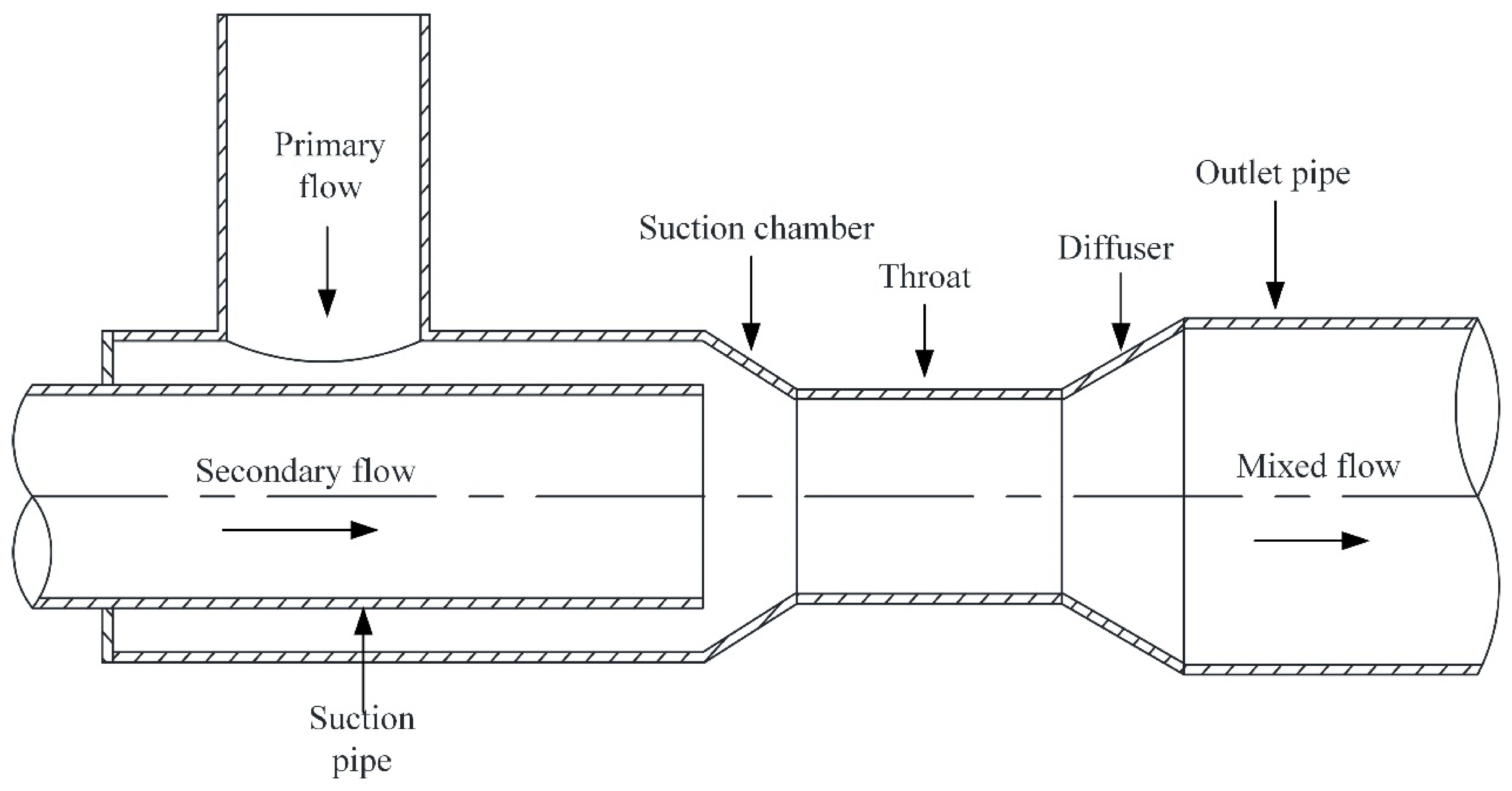
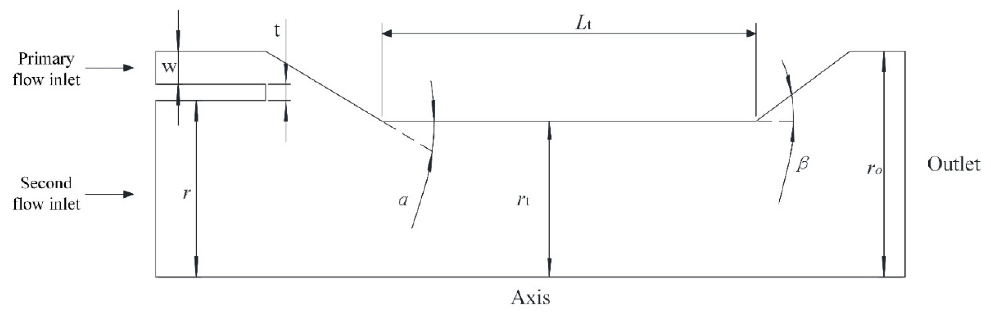
In this section, the CFD model is created and the simulation results are compared with the experiment results to verify the simulation. On the basis of the simulation method the parameters are optimized in the next section.

3.1. CFD Model

The annular jet pump calculation domain is shown in Figure 2. According to the existing research results [4], the initial model parameters are w = 4 mm, r = 21.5 mm, t = 2 mm, r₀ = 27.5 mm, r_t = 38 mm, α = 18°, L_t = 179 mm, β = 5.8°, m = 2.27. The sum of w, t and r equals r₀ in the optimization process. The wall thickness of suction pipe, t, is constant. Sheha [23] studied the performance over a large range of design parameters of jet pumps by a 2D simulation model. The result showed that the two-dimensional model still well simulated the flow field characteristics and jet pump performance of the actual model, ignoring the velocity in the z direction. Therefore, the 2D axisymmetric model was adopted in order to reduce the calculation cost. In the analysis and optimization of the jet pump, the suction angle α, the diffusion angle β and the area ratio m among the structural parameters—as shown in the Figure 2—plus the flow ratio q, are determined as the design variables.

The annular jet pump internal flow mechanism is complicated. The assumptions are made in CFD simulation for studying the jet pump:

(1)

the mixing process is considered as a steady and incompressible state;

(2)

the heat transfer of the external environment and the fluid medium is ignored;

(3)

the solid wall is considered smooth;

(4)

the buoyancy effect is ignored.

The continuity and momentum equations are listed as, because of these assumptions:

$$\frac{\partial \left(\rho u_i\right)}{\partial x_i}=0$$

(5)

$$\frac{\partial \left(\rho u_j{u}_i\right)}{\partial x_j}=\frac{\partial }{\partial x_j}\left[\mu \frac{\partial u_i}{\partial x_j}-\rho \overline{u_i{u}_j}\right]-\frac{\partial p}{\partial x_i}$$

(6)

where Reynolds stresses are

$$-\rho \overline{u_i{u}_j}={\mu }_t\left[\frac{\partial u_i}{\partial x_j}+\frac{\partial u_j}{\partial x_i}\right]-\frac{2}{3}\rho k{\delta }_{ij}$$

(7)

In these equations, u_i is velocity component, x_i is space coordinate, δ is boundary layer thickness, μ is dynamic viscosity, μ_t is turbulent viscosity, and k is turbulence kinetic energy.

Due to the jet pump internal flow complexity, it is necessary for ensuring the simulation accuracy to choose the appropriate turbulence model. The existing research [24] shows that standard wall function and the realizable k–ε model can accurately simulate annular jet pump flow details and calculate the performance index.

The realizable k–ε model [25] has advantages in simulating flow field details compared with the standard k–ε mode, such as vortices, and rotation. The modified transport equations for k and ε in the realizable k–ε model are:

$$\begin{array}{ll}\frac{\partial \left(\rho k\right)}{\partial t}+\frac{\partial \left(\rho k{u}_j\right)}{\partial x_j}=& \frac{\partial }{\partial x_j}\left[\left(\mu +\frac{\partial u_i}{{\sigma }_k}\right)\frac{\partial \left(k\right)}{\partial x_j}\right]\\ & +G_k+G_b-\rho \epsilon -Y_M+S_k\end{array}$$

(8)

$$\begin{array}{ll}\frac{\partial \left(\rho \epsilon \right)}{\partial t}+\frac{\partial \left(\rho \epsilon u_j\right)}{\partial x_j}=& \frac{\partial }{\partial x_j}\left[\left(\mu +\frac{\partial u_t}{{\sigma }_{\epsilon }}\right)\frac{\partial \epsilon }{\partial x_j}\right]+\rho C_{1}S\epsilon \\ & -\rho C_2\frac{{\epsilon }^2}{k+\sqrt{v\epsilon }}+C_{1\epsilon }\frac{\epsilon }{k}{C}_{3\epsilon }{G}_b+S_{\epsilon }\end{array}$$

(9)

where

$$C_1=\max \left[0.43,\frac{\eta }{\eta +5}\right],\eta =S\frac{k}{\epsilon },S=\sqrt{2S_{ij}{S}_{ij}}$$

(10)

In these equations, S is strain rate magnitude, G_k represents the generation of turbulence kinetic energy due to the mean velocity gradients. G_b is the generation of turbulence kinetic energy due to buoyancy. Y_m represents the contribution of the fluctuating dilatation in compressible turbulence to the overall dissipation rate. C₂ and C_ε are constants. σ_k and σ_ε are the turbulent Prandtl numbers for k and ε, respectively. S_k and S_ε are user-defined source terms.

The eddy viscosity is:

$${\mu }_t=\rho C_{\mu }\frac{k^2}{\epsilon }$$

(11)

Compared with the standard k–ε model, C_μ is no longer a constant in the realizable k–ε model and its formula is as follows:

$$C_{\mu }=\frac{1}{A_0+A_S\frac{k{U}^{\ast }}{\epsilon }}$$

(12)

and

$$\begin{array}{l}{U}^{\ast }\equiv \sqrt{S_{ij}{S}_{ij}+{\tilde{\mathsf{\Omega }}}_{ij}{\tilde{\mathsf{\Omega }}}_{ij}}\\ {\tilde{\mathsf{\Omega }}}_{ij}={\mathsf{\Omega }}_{ij}-2{\epsilon }_{ijk}{\omega }_k\\ {\mathsf{\Omega }}_{ij}={\overline{\mathsf{\Omega }}}_{ij}-{\epsilon }_{ijk}{\omega }_k\\ A_0=4.04,A_s=\sqrt{6}\cos \phi \\ \phi =\frac{1}{3}{\cos }^{-1}\left(\sqrt{6}W\right),W=\frac{S_{ij}{S}_{jk}{S}_{ki}}{{\tilde{S}}^3},\tilde{S}=\sqrt{S_{ij}{S}_{ij}},S_{ij}=\frac{1}{2}\left(\frac{\partial u_j}{\partial x_i}+\frac{\partial u_i}{\partial x_j}\right)\end{array}$$

(13)

where ${\overline{\mathsf{\Omega }}}_{ij}$ is the mean rate-of-rotation tensor. It can be concluded that C_μ is a function of the mean strain and rotation rates, the angular velocity of the system rotation, and the turbulence fields.

All fluids in the computational domain are water in this study. The grids of all the models are 2D unstructured grids and created by MESH. The mesh at the suction chamber inlet is refined. Velocity inlet boundary conditions are adopted for all fluid inlets. Turbulence specification method is given by turbulent intensity and hydraulic diameter. The outlet is set as outflow. All annular jet pump CFD simulations are conducted by the ANSYS Fluent R18.0 (Houston, PA, USA) which uses the finite volume method as a numerical solution technique. The pressure and velocity coupling method adopted the semi-implicit method for pressure linked equations (SIMPLE) algorithm with the pressure-based solver. The spatial discretization of the convection terms selected the second order upwind scheme.

All simulations are performed in parallel on a computer with an Inter Core (TM) i5-9400 CPU (6 processor, each with a clock speed of 2.9 GHz). The number of complete convergence iterations is 3000, and the computation time is 30 min per case. The contingent conditions in the CFD process are controlled to achieve strict consistency to ensure the reliability of the computation results. When the iteration converges, global scaled residuals for continuity and momentum equations drop to 10⁻⁶.

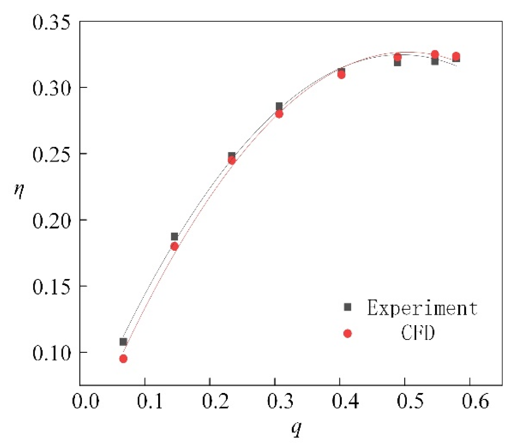
3.2. Verification of CFD Simulation

For verifying the reliability of the selected CFD model and algorithm used for further research on the annular jet pump, the simulation results are checked by the experiment data [4]. In this experiment, driving water pumped by a centrifugal pump flows into the chamber via the flow measuring orifice. The suction pipe included an electronic flowmeter. P_p, P_s and P_o are measured by mercury manometers. The performance of many pumps with different configurations is investigated for different jet quantities, while the suction height is kept constant. The model parameters are shown in the initial model. The comparison is as shown in Figure 3. It can be seen in Figure 3 that the numerical calculation results in this paper are in good agreement with the experimental data. The model selected in this paper accurately and reliably calculates the performance of the annular jet pump.

4. Hybrid Algorithm and Optimization Process

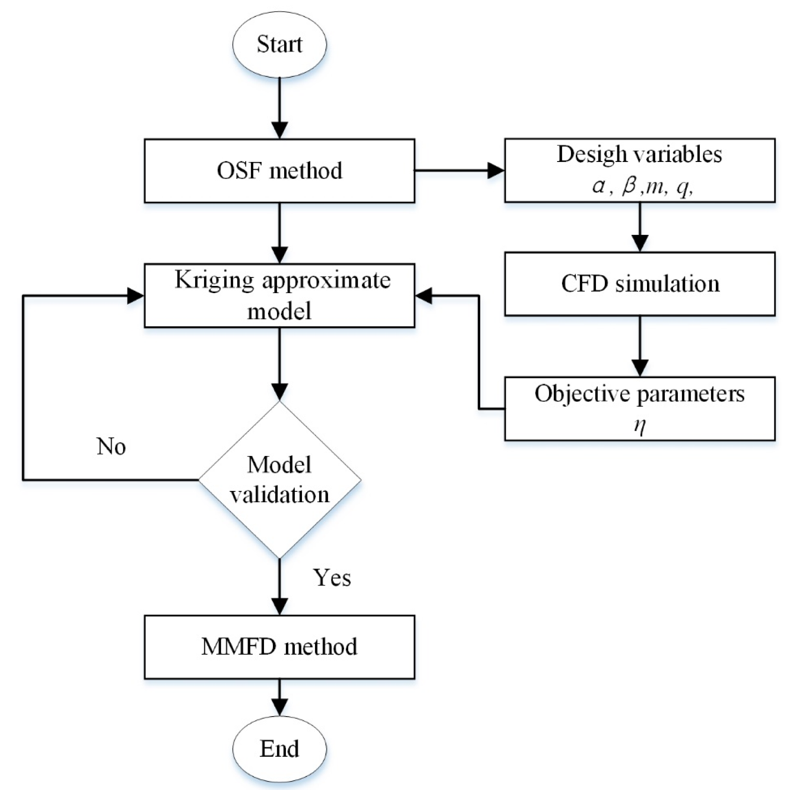
4.1. Optimization Algorithm Design

This paper proposes a hybrid algorithm for solving the global optimal solution. The algorithm selects the optimal space filling design (OSF) [26] experimental design method to obtain the global optimal point in the nonlinear optimization space, and adopts MMFD [27] to search and optimize the local in detail based on the Kriging approximate model [28]. Figure 4 is the hybrid algorithm optimization flow chart. The primary flow can be summarized as follows:

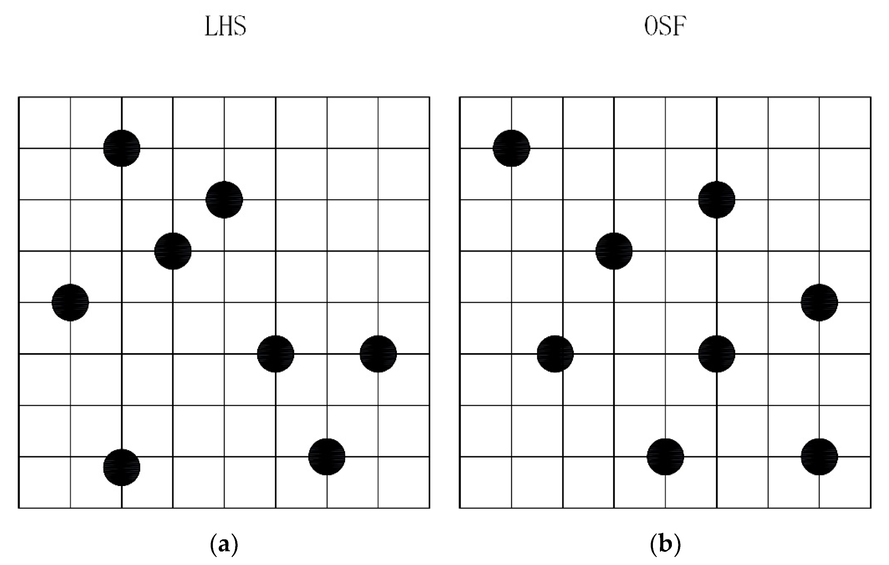
• In the design space, the space-filling sample points are generated by OSF.
• According to the sampling point, the CFD software Fluent is used to simulate the model with different structural parameters. Based on numerical simulation, the annular jet pump efficiency is evaluated.
• The Kriging approximate model is constructed by determining the type and parameters of the regression model. The structural parameters of the annular jet pump obtained at the sampling point in step one are input variables, and the efficiency η of the jet pump obtained in step two is the output variable.
• The Kriging approximate model constructed in step three is checked by analyzing the errors of the simulated values and the predicted values: if the error meets the requirements, transfer to step five; otherwise, transfer to step three and continue to update the Kriging model.
• Based on the Kriging approximate model, the MMFD is used to obtain the structural parameters optimal solution in the annular jet pump;
• According to the design parameters of the optimal solution, a physical prototype is generated. Then the CFD simulation and optimization results of the physical prototype are verified with each other.

4.2. Sampling Method

OSF is improved from Latin hypercube sampling algorithm (LHS). OSF improves the randomness of LHS so that all test points in the design space are distributed as uniformly as possible to assure a good space-filling and uniformity. Therefore, OSF is better to reflect the mapping information between the factors and the response, which makes the fitting more accurate with the minimum trials.

Figure 5a shows the sampling points distribution randomly obtained by Latin hypercube, and Figure 5b shows that the sampling points distribution uniformly generated by OSF. It can be seen that LHS lacks sample points in the upper right corner and cannot reflect the relationship between the factor and the response in this area. The use of OSF makes the sample points more uniform in the entire design space.

Rather than traditional algorithms, such as response surface methodology (RSM), central composite design (CCD), and factorial design, OSF is more suitable for computer-based deterministic meta models because of this advantage. This study generated sample points by OSF in the design space, ensuring the accuracy of the approximate model.

4.3. Approximate Model

The Kriging model is widely used in predicting spatially and temporally related data. It was originally used in geostatistics which is an interdisciplinary field of statistics, mathematics, geology, engineering and mining. Due to its stochastic assumption, the Kriging approximation is superior to traditional RSM in high dimensional nonlinear problems and high precision prediction [29]. The Kriging model is described by:

$$y\left(x\right)=f\left(x\right)+Z\left(x\right)$$

(14)

where y(x) is the unknown response function, f(x) is a known polynomial function of x called the trend, and Z(x) is a stochastic process with nonzero covariance, variance σ², and mean zero. The term of f(x) in the equation is similar to the polynomial model in a response surface, serving as a “global” model of the design space. In many cases, f(x) is taken to be a constant term β₀. When f(x) “globally” approximates the design space, Z(x) localized deviation, so the Kriging approximate model interpolates the sampling data points. The covariance matrix of Z(x) that represents the local deviations is:

$$Cov\left[Z\left(x_i\right),Z\left(x_j\right)\right]={\sigma }^2\mathrm{R}\left(\left[R\left(x_i,x_j\right)\right]\right)$$

(15)

where R is the correlation matrix, and R(x_i, x_j) is the correlation function between any two of the n_s sampled data points x_i and x_j. R is a [n_s × n_s] symmetric, positive definite matrix with ones along the diagonal. Many different correlation functions are available for the Kriging model, such as the linear correlation function, exponential correlation function and Matern Cubic correlation function. However, the Gauss correlation function is more popular in Kriging metamodels. The Gaussian correlation model is used in this paper, defined as:

$$R\left(\theta ,\omega ,x\right)=\exp \left(-{\displaystyle \sum _{j=1}^n{\theta }_j{\left({\omega }_j-x_j\right)}^2}\right)$$

(16)

where ω_j and x_j represent the jth component of sample points ω and x, respectively, θ_j is the unknown correlation parameters used to fit the model and n is the dimension of the design variable.

Once the correlation function has been selected and the best θ_j estimated, the Kriging model can be used to predict the response y (x) at an untried location x using:

$$\widehat{y}\left(x\right)=\widehat{\beta }+r^T\left(x\right)R^{-1}\left(Y-f\widehat{\beta }\right)$$

(17)

where, $\widehat{y}\left(x\right)$ is the vector of estimated response values at each sample point, $\widehat{\beta }$ is a constant, $r^T\left(x\right)$ is the vector of correlation values between the untried location x and the sample data points, and f is the vector with values of the trend function evaluated at each sample point.

$\widehat{\beta }$ can be calculated as

$$\widehat{\beta }={\left(f^T{R}^{-1}f\right)}^{-1}{f}^T{R}^{-1}Y$$

(18)

The estimate of the variance is

$${\widehat{\sigma }}^2=\frac{1}{n_s}{\left(Y-f\widehat{\beta }\right)}^T{R}^{-1}\left(Y-f\widehat{\beta }\right)$$

(19)

After selecting the form of the regression model and the correlation function, the correlation matrix R, the unknown parameter β₀, and σ² depend on the correlation parameter θ. Therefore, the Kriging metamodel can only be fully established after determining the value of θ. Maximum likelihood estimation (MLE) is a commonly used method for calculating related parameter values. This optimization can be translated into an unconstrained global optimization, as follows:

$$\{\begin{array}{c}Minimize\left\{\psi \left(\theta \right)=\sigma \left({\theta }^2\right){\left|R_{\theta }\right|}^{\frac{1}{n_s}}\right\}\hfill \\ Subjectto\hspace{1em}\hspace{1em}\theta >0\hfill \end{array}$$

(20)

4.4. Objectives and Constraints

The optimization of the jet pump in this study is a single objective optimization. In this paper, the limits applied to the optimization problem are based on reference [4]. The objective function is defined as:

$$\begin{array}{cc}Maximize& \eta =f\left(\alpha ,\beta ,m,q\right)\end{array}$$

(21)

Subject to:

$$\{\begin{array}{c}1.68\le m\le 7.18\\ 0.35\le q\le 0.8\\ {18}^{\circ }\le \alpha \le {60}^{\circ }\\ 4^{\circ }\le \beta \le {10}^{\circ }\end{array}$$

(22)

MMFD is a gradient optimization method which can solve optimizations with real variables. This method can quickly obtain the local optimal solution around the initial design point. It is very suitable for highly nonlinear design spaces. Therefore, the MMFD method is used in the study.

5. Results and Discussion

5.1. Results of Experimental Design

The structural parameters of 80 sample points are listed in

Table 1. Design parameters and efficiency of DOE sample points.

q	m	α (°)	β (°)
0.5835	4.256	20.22	9.164
0.7259	1.789	30.54	7.646
0.538	2.454	18.84	8.178
0.4013	4.078	20.5	8.936
0.3899	4.876	20.22	9.164
…	…	…	…
0.8	3.616	39.44	4.912
0.7146	5.675	18	5.518
0.4525	2.779	35.26	6.43
0.6405	2.347	39.72	6.354
0.4924	2.417	21.06	4.456

. Figure 6 shows the distribution of 80 samples. The best sample point is No. 52 (α = 27.74°, β = 4.76°, q = 0.4354, m = 1.84), and the corresponding jet pump efficiency is 0.332047. This sample point serves as the initial value of optimization.

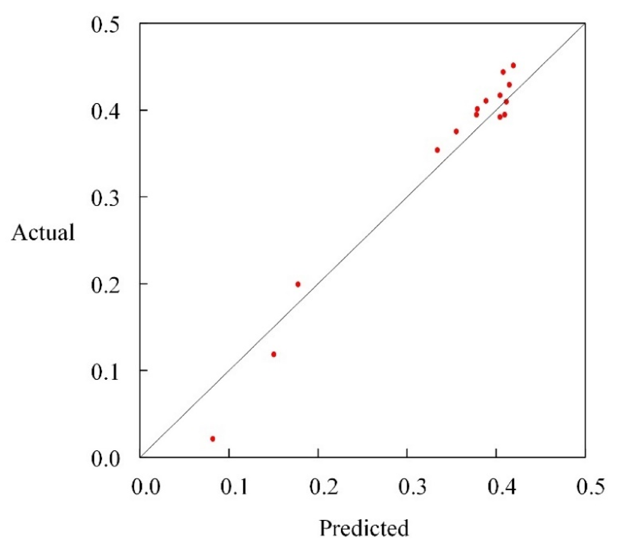
5.2. Approximate Model and Verification

The design variables of 80 sample points generated by the OSF and the corresponding CFD simulation results are used as inputs and outputs to establish a Kriging approximate model. Specifically, the parameters α, β, m and q of the jet pump are design parameters, and the corresponding efficiency η is the output variable.

Table 2. The Kriging model parameters.

Parameter	Value
β0	−0.0747
σ	0.06742
θ	(1.2707 1.201 0.5417 0.2051)

lists the parameters of the Kriging model. The model parameters are composed of β₀, σ and θ, where β is the regression model parameter and the others are the correlation model parameters. Figure 7 shows the degree of fitting between the predicted value of the objective function and the simulated value of CFD. On the diagonal, the predicted value is equal to the CFD value. It can be seen that all the points distribute about the diagonal.

For the sake of further verifying the Kriging modeling accuracy, a statistical measure of objective function, correlation coefficient is introduced for evaluating the approximate degree. The correlation coefficient R² is defined as follows:

$$R^2=1-\frac{{\displaystyle \sum _{i=1}^n{\left(y_i-Y\right)}^2}}{{\displaystyle \sum _{i=1}^n{\left(y_i-\overline{y}\right)}^2}}$$

(23)

The closer R² is to one, the better the fitting is. After calculation, R² is 0.9459.

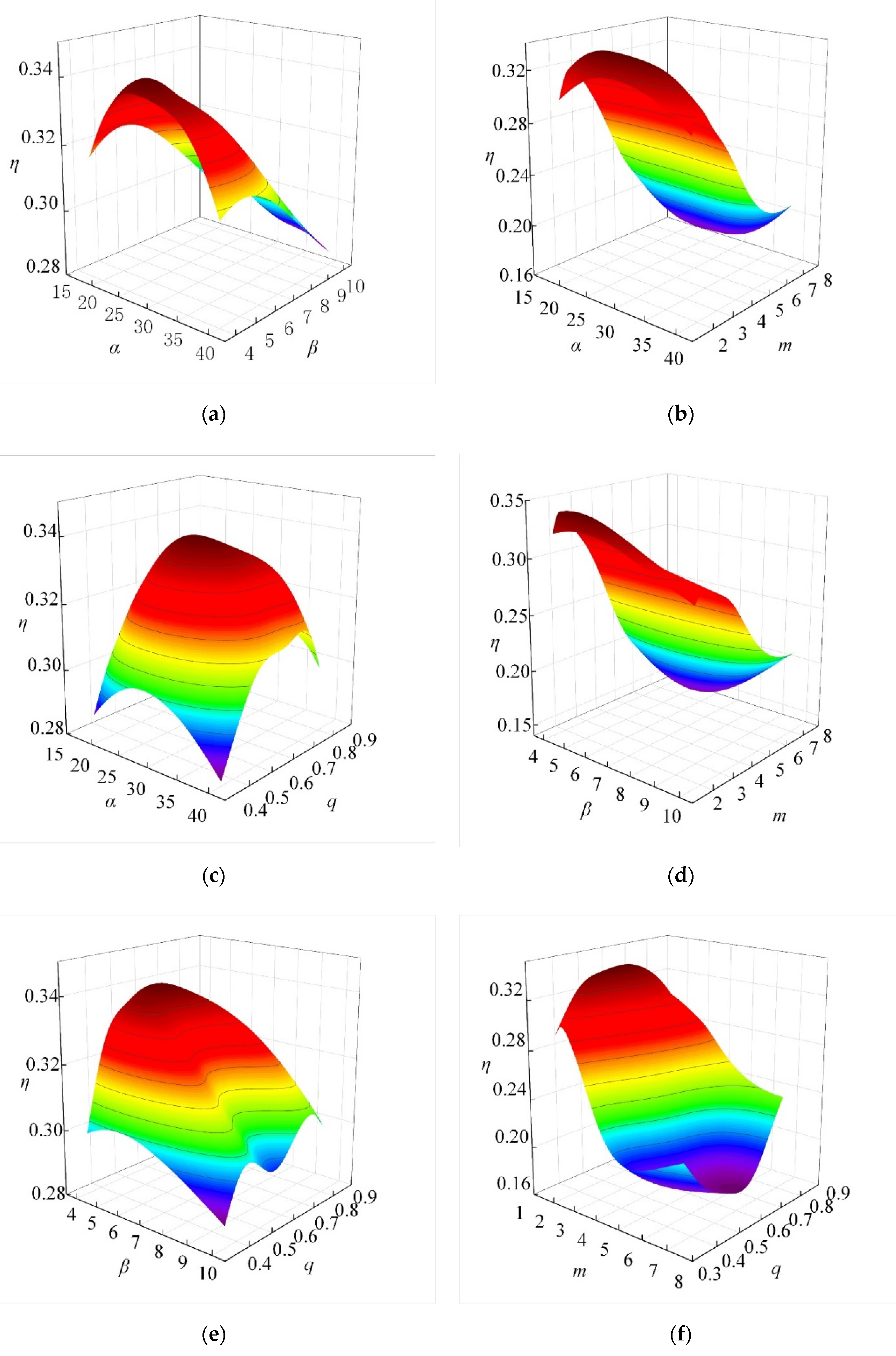
5.3. Response Surface Analysis

Kriging response surfaces are shown in Figure 8 to visualize the relationship between efficiency and various factors, where the efficiency η can reach a maximum of 33.89%. By comparing Figure 8a–c it can be seen that with the increase in the suction angle α, the efficiency curve of the jet pump is similar to a parabola; the efficiency reaches the maximum value with α = 26.6°, and the minimum values at boundaries (limits) of α. Comparing Figure 8a,d,e with the increase in the diffusion angle β, the jet pump efficiency curve approximates parabola as well; the efficiency reaches the maximum value with β = 4.12°, and the minimum value at the boundaries of β. Comparing Figure 8b,d,f it can be found that when the area ratio, m, increases, the efficiency of the jet pump increases first and then decreases by an S-curve trend; the efficiency reaches the maximum value with m = 2.11, and the minimum at the boundaries of m. Comparing Figure 8c,e,f when the flow ratio increases, the jet pump efficiency curve approximates a parabola and fluctuates (Figure 8e); the efficiency reaches the maximum with q = 0.6, and the minimum value at the boundaries of q, Figure 8c,e or at medium value of q, Figure 8f.

The peak efficiency does exist in the combination of parameters predicted by the approximate model. The optimal combination is: α = 26.6°, β = 4.12°, m = 2.11, q = 0.6. The efficiency calculated by CFD under this condition is 34.15%. The predicted value of the optimization algorithm is in good agreement with the value calculated by CFD.

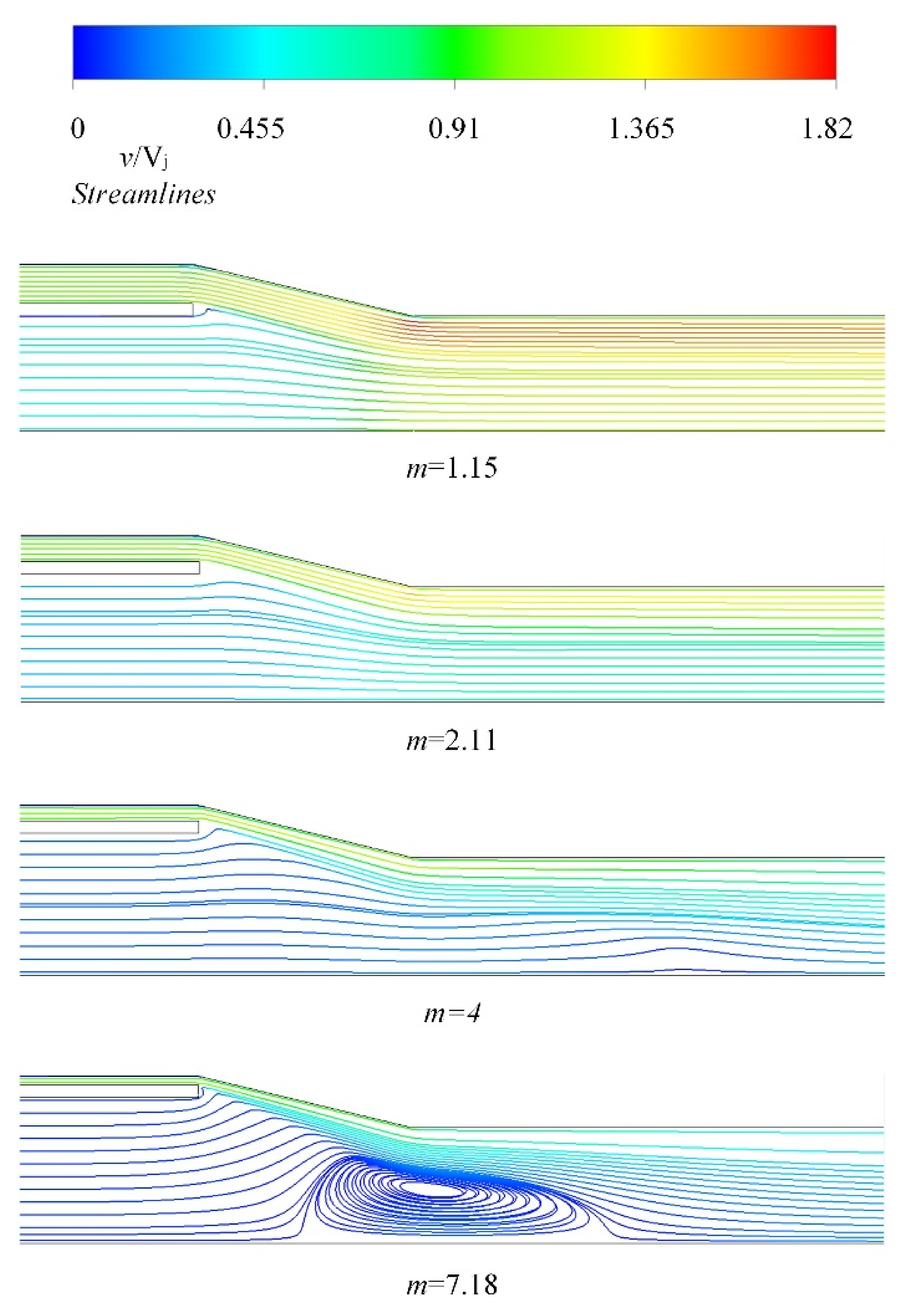
5.4. The Effect of m on Jet Pump

It can be concluded from the response surface analysis that m is very important for improving the efficiency of jet pumps. There have been many studies on other parameters rather than m. Figure 9 shows streamlines from the suction chamber to the inlet of the throat with different area ratios m = 1.15, 2.11, 4, 7.18 with α = 26.6°, β = 4.12°, and q = 0.6. A symmetrical vortex structure appears near the axis from the end of suction chamber to the inlet of throat at m = 7.18. This pair of vortices leads to the increase in friction resistance. Figure 10 shows the axial velocity profile of the throat inlet in order to further study this phenomenon.

As shown in Figure 10, the jet expands towards the center in the suction chamber. As m decreases, the jet expands deeper into the suction chamber. When the area ratio is 7.18, the jet fails to extend to the center and forms a back flow zone at the center. The smaller the area ratio is, the better the mixing effect of the jet at the outlet of the suction chamber is.

Figure 11 shows the annular jet pump velocity distribution with the above four area ratios. The velocity gradient of the high-speed jet and the sucked second fluid in the suction chamber is relatively big, and the degree of mixing of the two fluids is low. Because the jet expands unilaterally, the jet velocity is high in the suction chamber near the side wall of the throat, and the velocity gradient is big. As the area ratio decreases, the energy loss of the jet increases in the suction chamber and the throat. Therefore, a low area ratio leads to a small inlet of primary fluid and high friction resistance and reduces the efficiency of the annular jet pump.

6. Conclusions

In this paper, an optimization method based on the Kriging model and MMFD is used to obtain the maximum efficiency which is closer to the global optimal solution and to solve the constrained optimization problem with a given head ratio by building the functional relationship between efficiency and design parameters, which makes the method more applicable. The CFD simulation scheme is created and verified with experiment data, which ensures the reliability of the simulation results. Based on the sampling points generated by the OSF method, a Kriging approximate model is established, and the accuracy of the Kriging approximate model is verified by CFD simulation results. To the end, the parameters of the annular jet pump are optimized with the MMFD algorithm.

According to the results above, the following conclusions can be drawn:

(1)

The R² of the Kriging approximate model constructed based on OSF sampling method is more than 0.9, so the proposed modeling method meets the accuracy requirements.

(2)

The optimal efficiency of the annular jet pump is 33.89% predicted in optimization and 34.15% by simulation with the combination of pump parameters: α = 26.6°, β = 4.12°, m = 2.11, q = 0.6.

(3)

The area ratio m is a key parameter affecting the efficiency of the jet pump, and an analysis of the flow field and performance with different m was performed. By decreasing the area ratio, m, the jet mixing effect at the outlet of the suction chamber can be improved, but leads to the frictional resistance increase. In this case the optimal value of m is 2.11.

References

1. Yapıcı, R.; Aldas, K. Optimization of water jet pumps using numerical simulation. Proc. Inst. Mech. Eng. Part A J. Power Energy 2013, 227, 438–449. [Google Scholar] [CrossRef]
2. Meakhail, T.; Teaima, I. Experimental and numerical studies of the effect of area ratio and driving pressure on the performance of water and slurry jet pumps. Proc. Inst. Mech. Eng. Part C J. Mech. Eng. Sci. 2012, 226, 2250–2266. [Google Scholar] [CrossRef]
3. Long, X.; Xu, M.; Wang, J.; Zou, J.; Bin, J. An experimental study of cavitation damage on tissue of Carassius auratus in a jet fish pump. Ocean Eng. 2019, 174, 43–50. [Google Scholar] [CrossRef]
4. Shimizu, Y.; Nakamura, S.; Kuzuhara, S. Studies of the Configuration and Performance of Annular Type Jet Pumps. J. Fluid Eng. 1987, 3, 205–212. [Google Scholar] [CrossRef]
5. Kwon, O.B.; Kim, M.K.; Kwon, H.C.; Bae, D.S. Two-dimensional Numerical Simulations on the Performance of an Annular Jet Pump. J. Vis. Jpn. 2002, 5, 21–28. [Google Scholar] [CrossRef]
6. Long, X.; Yan, H.; Zhang, S.; Yao, X. Numerical simulation for influence of throat length on annular jet pump performance. J. Drain. Irrig. Mach. Eng. 2010, 3, 198–201. [Google Scholar] [CrossRef]
7. Yang, X.; Long, X.; Yao, X. Numerical investigation on the mixing process in a steam ejector with different nozzle structures. Int. J. Therm. Sci. 2012, 56, 95–106. [Google Scholar] [CrossRef]
8. Lyu, Q.; Xiao, Z.; Zeng, Q.; Xiao, L.; Long, X. Implementation of design of experiment for structural optimization of annular jet pumps. J. Mech. Sci. Technol. 2016, 30, 585–592. [Google Scholar] [CrossRef]
9. Deng, X.; Dong, J.; Wang, Z.; Tu, J. Numerical analysis of an annular water–air jet pump with self-induced oscillation mixing chamber. J. Comput. Multiph. Flows. 2017, 9, 47–53. [Google Scholar] [CrossRef]
10. Xiao, L.; Long, X.; Lyu, Q.; Hu, Y.; Wang, Q. Numerical Investigation on the Cavitating Flow in Annular Jet Pump under Different Flow Rate Ratio; Symposium on Hydraulic Machinery and Systems (IAHR): Montreal, QC, Canada, 2014. [Google Scholar] [CrossRef] [Green Version]
11. Xu, M.; Yang, X.; Long, X.; Lyu, Q. Large eddy simulation of turbulent flow structure and characteristics in an annular jet pump. J. Hydrodyn. 2017, 2, 702–715. [Google Scholar] [CrossRef]
12. Zou, C.H.; Li, H.; Tang, P.; Xu, D.H. Effect of Structural Forms on the Performance of a Jet Pump for A Deep Well Jet Pump. Computational Methods and Experimental Measurements XVII. In Proceedings of the International Conference on Computational Methods and Experimental Measurements 17th, Opatija, Croatia, 5–7 May 2015. [Google Scholar] [CrossRef] [Green Version]
13. Barthelemy, J.; Haftka, R. Approximation concepts for optimum structural design—A review. Struct Multidiscip. Optim. 1993, 5, 129–144. [Google Scholar] [CrossRef]
14. Gholap, A.; Khan, J. Design and multi-objective optimization of heat exchangers for refrigerators. Appl. Energ. 2007, 84, 1226–1239. [Google Scholar] [CrossRef]
15. Alexandras, A. Stochastic subset optimization incorporating moving least squares response surface methodologies for stochastic sampling. Adv. Eng. Softw. 2012, 44, 3–14. [Google Scholar] [CrossRef]
16. Verstraete, T.; Alsalihi, Z.; Braembussche, R. Multidisciplinary Optimization of a Radial Compressor for Microgas Turbine Applications. J. Turbomach. 2010, 132, 031004. [Google Scholar] [CrossRef]
17. Naseri, M.; Othman, F. Determination of the length of hydraulic jumps using artificial neural networks. Adv. Eng. Softw. 2012, 48, 27–31. [Google Scholar] [CrossRef]
18. Frédéric, M.; Luis, A.; Ichiro, H. Efficient preconditioning for image reconstruction with radial basis functions. Adv. Eng. Softw. 2007, 38, 320–327. [Google Scholar] [CrossRef]
19. Sun, H.; Schafer, M. Reduced order model assisted evolutionary algorithms for multi-objective flow design optimization. Eng. Optimiz. 2011, 43, 97–114. [Google Scholar] [CrossRef]
20. Zhang, Y.; Hu, S.; Wu, J. Multi-objective optimization of double suction centrifugal pump using Kriging metamodels. Adv. Eng. Softw. 2014, 74, 16–26. [Google Scholar] [CrossRef]
21. Safikhani, H.; Khalkhali, A.; Farajpoor, M. Pareto Based Multi-Objective Optimization of Centrifugal Pumps Using CFD, Neural Networks and Genetic Algorithms. Eng. Appl. Comp. Fluid. 2011, 5, 37–48. [Google Scholar] [CrossRef] [Green Version]
22. Zhao, A.; Lai, Z.; Wu, P. Multi-objective optimization of a low specific speed centrifugal pump using an evolutionary algorithm. Eng. Optimiz. 2016, 48, 1251–1274. [Google Scholar] [CrossRef]
23. Sheha, A.A.A.; Nasr, M.; Hosien, M.A.; Wahba, E.M. Computational and Experimental Study on the Water-Jet Pump Performance. J. Appl. Fluid Mech. 2018, 11, 1013–1020. [Google Scholar] [CrossRef]
24. Yang, X.; Long, X.; Xiao, L.; Lu, Q. Influence of different turbulence models on simulation of internal flow field of jet pump. J. Drain. Irrig. Mach. Eng. 2013, 31, 98–102. [Google Scholar] [CrossRef]
25. Shih, T.; Liou, W.; Shabbir, A.; Yang, Z.; Zhu, J. A new k-ε eddy viscosity model for high reynolds number turbulent flows. Comput. Fluids 1995, 24, 227–238. [Google Scholar] [CrossRef]
26. Jin, R.; Chen, W.; Sudjianto, A. An efficient algorithm for constructing optimal design of computer experiments. J. Stat. Plan. Infer. 2005, 134, 268–287. [Google Scholar] [CrossRef]
27. Vanderplaats, G. An efficient feasible directions algorithm for design synthesis. AIAA J. 1984, 22, 1633–1640. [Google Scholar] [CrossRef]
28. Simpson, T.; Mauery, F.; Korte, J.; Mauery, T. Comparison of Response Surface and Kriging Models for Multidisciplinary Design Optimization. In Proceedings of the Symposium on Multidisciplinary Analysis and Optimization (AIAA), St. Louis, MO, USA, 2–4 September 1998. [Google Scholar] [CrossRef]
29. Matta, A.; Pezzoni, M.; Semeraro, Q. A Kriging-based algorithm to optimize production systems approximated by analytical models. J. Intell. Manuf. 2012, 23, 587–597. [Google Scholar] [CrossRef]
Figure 1. Structural schematic drawing of annular jet pump.
Applsci 10 07860 g001
Figure 2. The calculation domain.
Applsci 10 07860 g002
Figure 3. Experiment and simulation data. CFD: computational fluid dynamics.
Applsci 10 07860 g003
Figure 4. The optimization flow. MMFD: modified method of feasible directions; OSF: optimal space filling design.
Applsci 10 07860 g004
Figure 5. Design of experiments (DOE) method. (a) Latin hypercube sampling algorithm (LHS); (b) OSF.
Applsci 10 07860 g005
Figure 6. Distribution of different sampling points. (a) α and β; (b) q and m.
Applsci 10 07860 g006
Figure 7. Error analysis of Kriging model.
Applsci 10 07860 g007
Figure 8. Response surface of efficiency. (a) α and β; (b) α and m; (c) α and q; (d) β and m; (e) β and q; (f) m and q.
Applsci 10 07860 g008
Figure 9. Streamlines from the suction chamber to the inlet of throat.
Applsci 10 07860 g009
Figure 10. The axial velocity profile of the throat inlet.
Applsci 10 07860 g010
Figure 11. Velocity field of jet pump with different m.
Applsci 10 07860 g011