The Significance of Sky Temperature in the Assessment of the Thermal Performance of Buildings

Abstract

Energy-efficient building design needs an accurate way to estimate temperature inside the building which facilitates the calculation of heating and cooling energy requirements in order to achieve appropriate thermal comfort for occupants. Sky temperature is an important factor for any building assessment tool which needs to be precisely determined for accurate estimation of the energy requirement. Many building simulation tools have been used to calculate building thermal performance such as Autodesk Computational Fluid Dynamics (CFD) software, which can be used to calculate building internal air temperature but requires sky temperature as a key input factor for the simulation. Real data obtained from real-sized house modules located at University of Newcastle, Australia (southern hemisphere), were used to find the impact of different sky temperatures on the building’s thermal performance using CFD simulation. Various sky temperatures were considered to determine the accurate response which aligns with a real trend of buildings’ internal air temperature. It was found that the internal air temperature in a building keeps either rising or decreasing if higher or lower sky temperature is chosen. This significantly decreases the accuracy of the simulation. It was found that using the right sky temperature values for each module, Cavity Brick Module (CB) Insulated Cavity Brick Module (InsCB), Insulated Brick Veneer Module (InsBV) and Insulated Reverse Brick Veneer Module (InsRBV), will result in 6.5%, 7.1%, 6.2% and 6.4% error correspondingly compared with the real data. These errors mainly refer to the simulation error. On the other hand using higher sky temperatures by +10 °C will significantly increase the simulation error to 16.5%, 17.5%, 17.1% and 16.8% and lower sky temperature by +10 °C will also increase the error to 19.3%, 22.6%, 21.9% and 19.1% for CB, InsCB, InsBV and InsRBV modules, respectively.

1. Introduction

The building sector contributes to climate change where energy usage in constructing and operating buildings account for 40% of the global energy use [1] and 32% of greenhouse gas (GHG) emissions [2]. Ways to decrease GHG emissions and save energy play an important role in designing energy-efficient structures. Energy supply, the increasing demands for energy, climate change, and the imperative to reduce greenhouse gas emissions must be considered in designing buildings. In order to design energy-efficient buildings, there should be accurate information about the thermal performance of the buildings. Energy-efficient buildings are vital as they reduce the consumption of energy and allow sustainable development. Erecting such buildings will require correct and realistic prediction of the buildings’ performance when subjected to a wide variety of harsh weather conditions in order to have a view of the impact of all the elements that influence the thermal performance such as the correct sky temperatures. The lack of specific sky temperature equations for all areas of the world makes it impossible to determine the best existing formula but the comparison among the models can be useful to address the choice of users in building energy simulations and engineering applications.

From the beginning of the 20th century, several researchers have focused their efforts on sky temperature models. Such models are associated with local weather patterns and particular locations. Hence, the extant differences between the models have been significant factors in the process of developing new models for various sites. The current models do not encapsulate the entire planet despite the fact that assessing sky temperature is required for evaluating the net radiative transfer of heat between surfaces and the sky vault. Therefore, taking into account the energy performance of buildings, radiative cooling and different engineering purposes, determining the sky temperature is critical and must be suitably accounted for.

The Earth is heated by radiation emitted by the Sun, which causes the release of adsorbed energy in the form of infrared thermal radiation that is detected as heat. This is a critical process due to the fact that if the adsorbed energy was not emitted by the Earth, temperatures would increase excessively, and the conditions on the planet would be too extreme to support life [3]. With no atmosphere, the majority of the radiation absorbed during the daytime would then be emitted in the direction of the sky in the night-time, which would make the Earth extremely cold. It is fortunate that there is an abundance of water vapour in the atmosphere, which is capable of absorbing a certain amount of the infrared rays radiating from the surface underneath. As a result of water vapour and additional greenhouse gases, the surface of the Earth is sufficiently warm to support life [4].

Although temperatures in outer space are roughly 3K, measurements of the sky overhead reveal a different story: this is due to water vapour contained within the atmosphere, which is warmed by the absorption of water vapour released by the ground below. The process by which the Earth is warmed by water vapour is defined as the greenhouse effect. The infrared element of the Sun’s radiation is partly trapped and then adsorbed by water vapour, thus causing the atmosphere to be warmed. Furthermore, the greenhouse effect is also exacerbated by other gases including methane and carbon dioxide, among others, which along with water vapour are acknowledged to be greenhouse gases [5]. The transferral of heat from a building’s outside surface and its environment is dependent on convective and radiative phenomena. Such mechanisms have been considered for many years via the usage of an effective outdoor air temperature known as sol-air temperature [3].

Heat transfer linked with sky longwave radiation is associated with an effective sky temperature and today the simulation of buildings’ energy performance involves models capable of estimating the temperature of the sky. The exchange of the sky longwave radiation is a function of the effective sky temperature. In the context of buildings, radiative cooling is caused by lost heat through the emission of longwave radiation in the direction of the sky, where the sky can be considered as a heat sink for outdoor services. Radiative cooling peaks at night when there are clear skies and reduced humidity [6].

It is widely acknowledged that electromagnetic radiation is emitted by all bodies in a wavelength range that is a function of their temperature and, in ambient conditions, the majority of the energy release occurs in the infrared range. The radiative cooling approach is aimed at establishing a cooling net balance between the thermal radiation emitted by ground level surfaces and the atmosphere. With regard to buildings, radiative cooling is a passive approach to cooling that exploits thermal radiation attributes to cool an object or areas of a building that face a colder surface, like the sky [7]. Such observations are purely linked with the construction sector, where nearly half of the energy demands of buildings are attributed to the need to air-condition living spaces. Additionally, the energy needs of buildings are growing, particularly in developing nations [8,9,10]. The construction industries of numerous countries need significant reform [11], and engineers and researchers deal with complex codes for the purpose of simulating the energy demands of buildings, analysing the manner in which the building interacts with internal and external environments [12], one aspect of which is represented by radiative heat exchange between the surfaces of the building and the sky vault. For such heat transfers to be evaluated, it is necessary to assess sky emissivity and temperature. From the beginning of the 20th century onwards, numerous researchers have focused on sky temperature models with studies proposing distinct relationships [13].

Sky models are associated with local weather patterns and particular locations. Hence, the extant differences between the models have been critical in the development of new models for various sites over the years [14,15]. Generally, large areas of the world are not covered by the existing sky models. Researchers have suggested various relationships in the literature and the majority of these models have been approximated because of insufficient accurate measured data.

The form and degree of complexity of the current models differ considerably. More data and research are required to include additional variables and facilitate improved predictions of sky temperature, accounting for factors like daily cycles or hourly fluctuations that occur independent of location and that can explain phenomena like dust storms or smog that exceeds cloudiness. Considering the effect of distinct relationships when simulating the energy performance of buildings, it was determined that the yearly energy demands from heating and cooling can be influenced by high percentage differences, which range between −10% and 19% for tropical environments, −10% and 13% for dry climatic environments, −19% and 28% for mild temperature environments and, lastly, between −43% and 83% for snowy environments (the latter percentage range is significantly higher than the others as it denotes virtually negligible energy demands for cooling) [16].

The universe is a perfect heat sink as its temperature is about 3 kelvin. However, at night, objects on the ground cool down due to the radiative emission to space. At daytime, the effect is negligible because solar irradiation heats up surfaces much more [17].

When radiation hits a surface it is partly reflected, partly absorbed (or transmitted). The absorbed radiation induces heat into the material. Every material with a temperature above 0 kelvin also emits thermal radiation. Therefore, the emissivity of an object is equal to the absorptivity at each wavelength and this is because of the low sky temperature. The temperature in external space close to absolute zero kelvin (−273.15 °C) reliant on the season and location, sky temperature from the earth will be near or below zero degrees celsius. The difference is mainly by water vapour in the sky that has become warm by absorbing infrared radiation emitted by the Earth. The warmed water vapour returns some of the infrared back to the Earth, and this helps keep the Earth warmer than space. Almost all the water vapour in the atmosphere is found in the troposphere, the layer of the atmosphere between the surface and around 10 km where there is no water vapour in stratosphere [18].

Sky temperature can be simplified as an average of the temperature between the ground and the upper troposphere where there is less water vapour. Therefore, the sky temperature is not the temperature of the sky but a number that indicates that the sky is much warmer than space and cooler than near the Earth. One of the methods to measure the sky temperature was by a weather balloon launched from Del Rio, Texas, on 21 September 2008 (altitude about 277 km away from earth surface) [18]. The temperature decreases sharply until an altitude of about 17,500 m, the temperature then begins to rise, this change marks the tropopause, the border between the troposphere (which is where most water vapour resides) and the very dry stratosphere above. The temperature increase in the stratosphere is caused by the ozone layer, which is warmed when it absorbs ultraviolet sunlight [18].

Several studies have been conducted on sky temperature models on the building’s thermal performance. These models are associated with local weather conditions and specific sites. As a result, the existing discrepancies between the models have been an essential factor for the improvement of new models for different locations and climates. The current models do not cover all climates and a location despite sky temperature calculation is necessary to assess the radiative heat transfer between the building and the sky dome. Consequently, considering building thermal performance, the calculation of sky temperature is vital and needs to be undertaken precisely.

It is worth noting that most of the sky temperature models are approximated due to the lack of accurate measured data [19]. Sky temperature models are related to local weather conditions and specific sites. Therefore, the existing deviations between the models have been a key factor for developing new models for different locations over the years. In general, the current sky temperature models do not cover most of the locations and climates around the world. Different relationships have been suggested over the years but most of these models are approximated due to the absence of detailed measured data.

It is worth mentioning that the sky temperature and ambient temperature are different. Temperatures tend to decrease from the ground going skyward, with a resulting sky temperature lower than the air temperature [20]. Moreover, the difference between sky and air temperatures is higher during the summer, especially during clear sky conditions.

There are many building thermal simulation software used in building thermal simulation such as TRNSYS (Transient System Simulation Tool) which specializes in complete solar energy system modelling while computational fluid dynamics (CFD) can be used in a wide range of building design from building site layout design to individual room planning and also can be used for active heating, ventilating and air-conditioning (HVAC) system design to passive ventilation study, consistent indoor air quality valuation, and serious fire smoke and toxin control [21].

The evaluation of the effect of sky temperature is relevant to building annual energy requirements. Consequently, a sample building was evaluated for the purpose of investigating the effects of various sky temperatures on the energy demands associated with cooling and heating. A comparison was made between the findings and the results detected on location. In this paper we undertake a demonstration of the effect of sky temperature in a moderate climate zone for different seasons and various housing modules using CFD simulation.

The paper is structured as follows: Section 2 provides an overview of the materials and methods used in this analysis including; 2.1 full scale test modules; 2.2 CFD analysis; 2.3 temperature boundary conditions and in Section 2.4 provides a brief description of the calculation of sky temperature used in this analysis. Section 3 gives the results and a discussion of different sky temperatures for all of the modules; finally, Section 4 provides the conclusions.

2. Materials and Methods

To find the effect of sky temperature on buildings simulations analysis performed using real data obtained from real-sized house modules compared with CFD simulated results for the exact same house module using different sky temperatures [22].

2.1. Full-Scale Test Modules

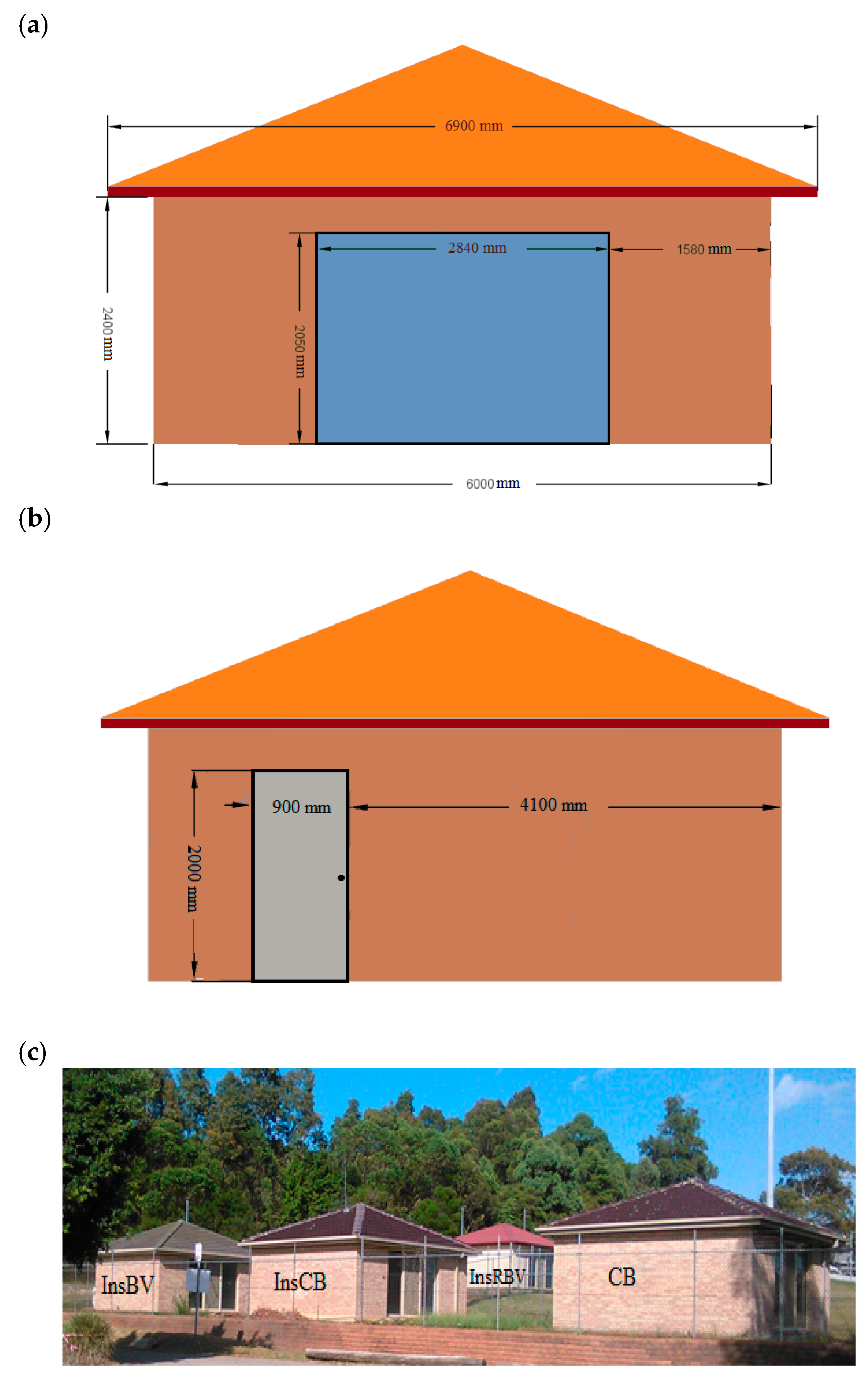
An ongoing research study is being conducted in the Priority Research Centre for Energy at the University of Newcastle in Australia to evaluate the thermal performance of houses in the country. In this program, four full-scale housing modules have been constructed and their thermal performance is monitored according to different weather states.

The construction of each of the models was performed on the Callaghan Campus of the University of Newcastle (longitude 151.7 E and latitude 32.9 S). The selection of the models was intended to ensure that they were representative of standard types of construction found in Australia [23]. The modules were separated at a distance of 7 m to diminish wind obstruction and prevent shading, and the design of all modules was identical consisting of a square floor plan with dimensions of 6 m × 6 m, as illustrated in Figure 1 [22].

The building materials in each of the modules included the following:

Window: Clear laminated glass with a thickness of 6.38 mm with a light-coloured aluminium frame situated in the northern wall of every module.

Door: To allow the modules to be accessed, doors with high quality insulation were fabricated in the southern wall to ensure that heat losses were reduced and that the modules could be entered.

Roof: Each roof was constructed from concrete and clay tiles with sarking insulation. Between the rafters, a 10 mm plasterboard ceiling was installed with R3.5 glass wool batts insulation.

Slab: The entire building floor was covered by a concrete slab with a thickness of 100 mm.

The modules were all designed in the same way with identical construction materials apart from the walling systems; consequently, the naming of the modules is based on the walling system used in the construction [22].

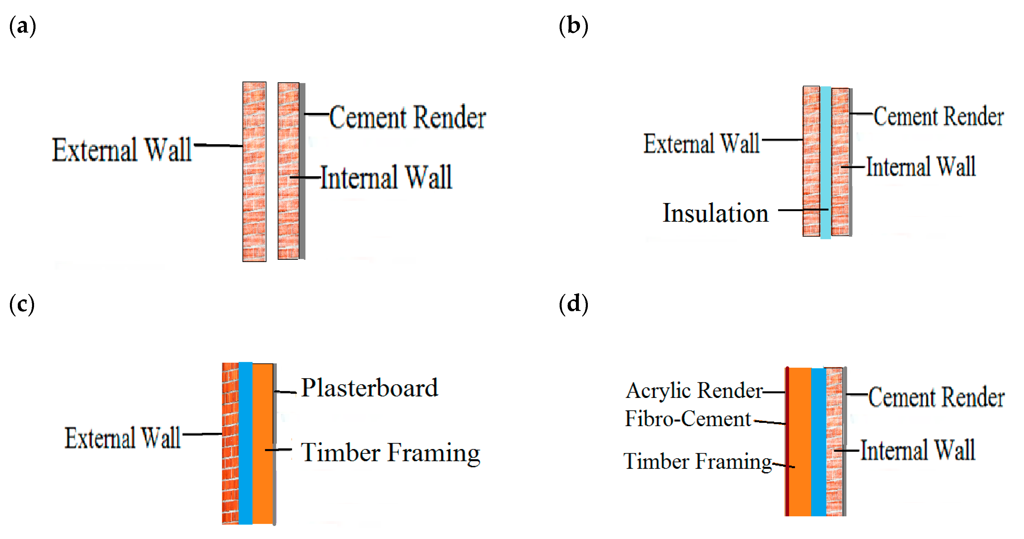
Cavity Brick Module (CB); The CB module walling comprised a pair of 110 mm brickwork skins separated by a 50 mm cavity and a 10 mm render covering the inside walls, as illustrated in Figure 2a.

Insulated Cavity Brick Module (InsCB); The InsCB module has two 110 mm brickwork skins divided by a 50 mm cavity containing R1 polystyrene insulation, and the inside walls are coated in a 100 mm internal render, as illustrated in Figure 2b.

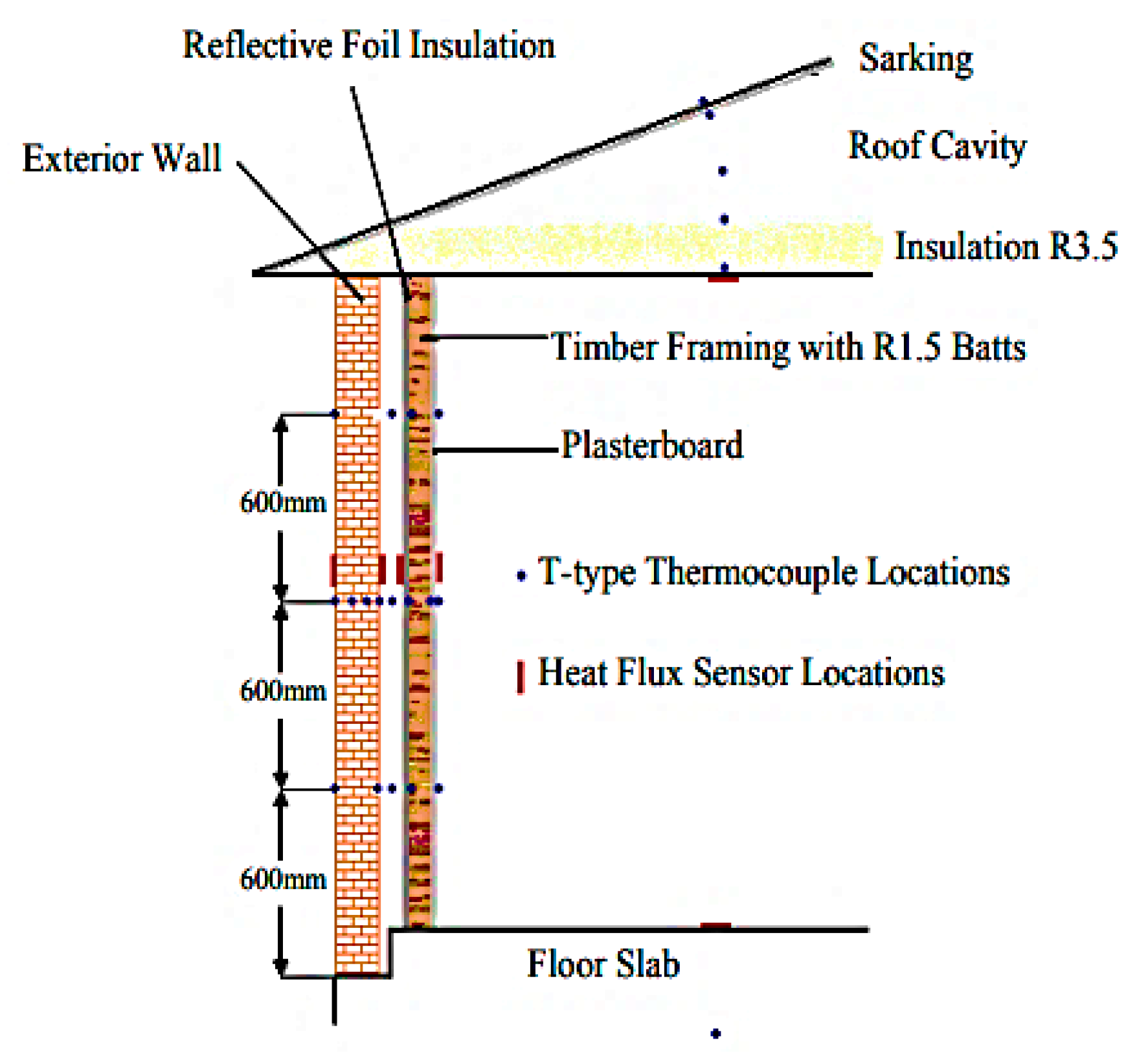
Insulated Brick Veneer Module (InsBV) In the InsBV module, the inside walls comprised an internal frame constructed from timber with low-glare reflective foil and R1.5 glass wool batts covered by 10 mm plasterboard; the outside walls were fabricated utilising a 110 mm brickwork skin, as demonstrated in Figure 2c.

Insulated Reverse Brick Veneer Module (InsRBV) For the inside walls, a 10 mm internal render covers a 110 mm brick skin. The outside walls consist of a 2–3 mm acrylic render on 7 mm fibro-cement sheets attached to a timber stud frame with R1.5 glass wool batts insulation, as illustrated in Figure 2d.

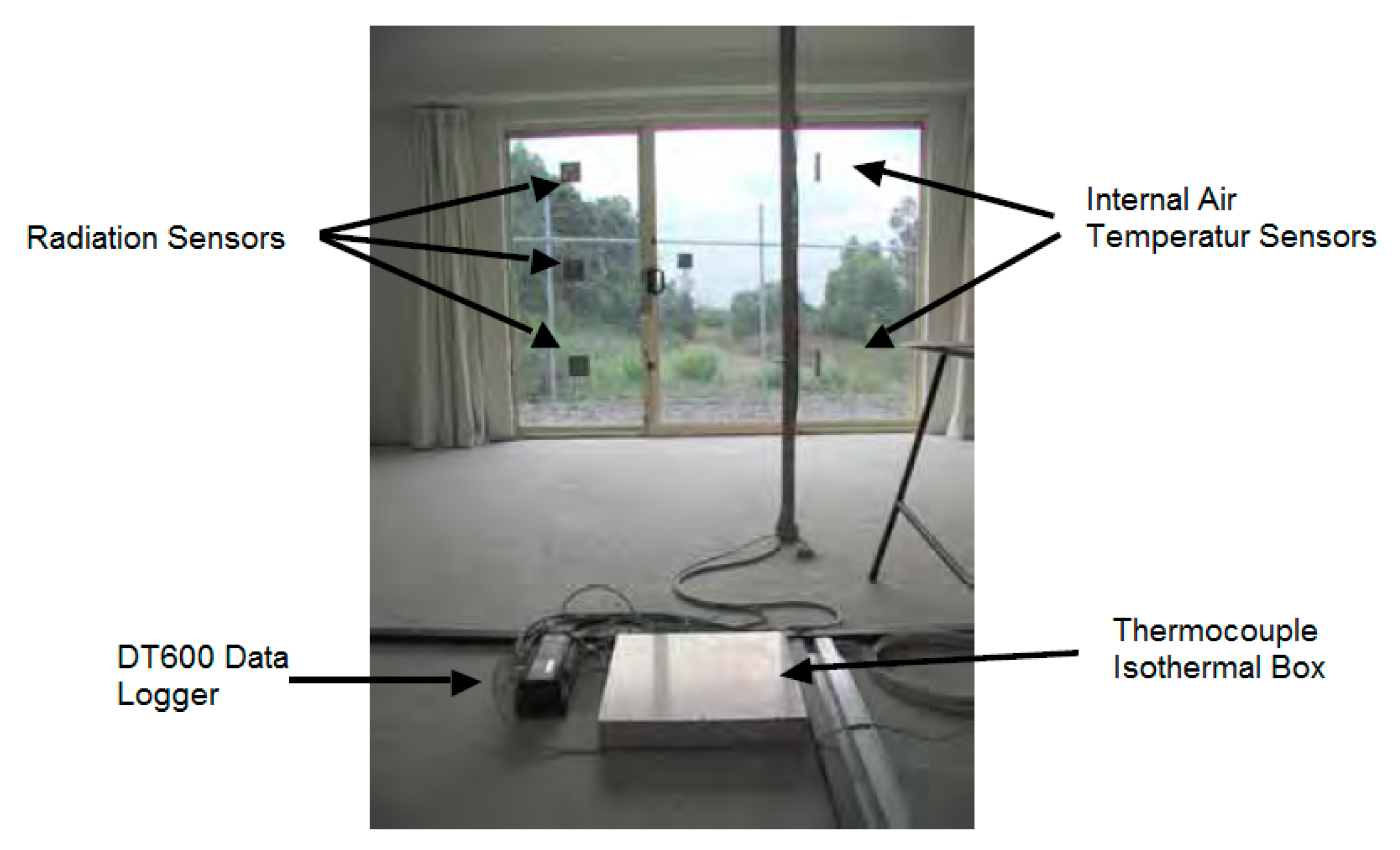
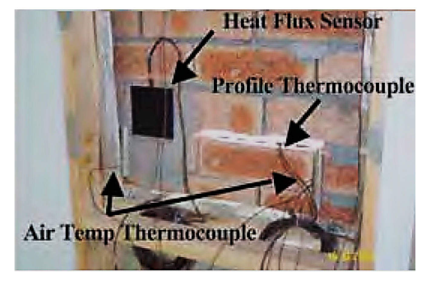
For each module, in excess of 100 sensors were placed for the purpose of recording the outside weather conditions as well as the inside environment; data recording was performed at 5 min intervals throughout the testing period utilizing Datataker DT600. The air temperature within each of the “free-floating” modules with no mechanical heating or cooling will be specifically determined by the outside weather conditions. None of the models were ventilated and the inside air temperature was recorded at an elevation of 1200 mm within the structures [24].

Amended to the Section 2.1 “Full-Scale Test Modules”

The sensors were installed in each module with a minimum of 40 sensors as required by ASHRAE55 to measure the thermal comfort performance of a small room. The sensors were distributed on the walls and in the middle of the module away from the occupied boundary, radiation, and diffusers (See Figure 3 and Figure 4). The data were recorded using Datataker DT600 data loggers every 5 min for 24 h/day over the testing period [24].

In this research, the operative temperature was calculated by finding the average air temperature for the sensors located in the middle of the building at different heights: 600 mm, 1200 mm, and 1800 mm. Typical sensor arrangements are shown schematically in Figure 5 for each of the wall types [24].

Considering the thermal exchange that occurs between buildings and the environment, in the absence of data to calculate sky temperature, this can be easily calculated using ISO 13790, as demonstrated by the equations shown below [25]:

• T_sky = T_amb − 11 (Temperate areas)
• T_sky = T_amb − 9 (Sub-polar areas)
• T_sky = T_amb − 13 (Tropical areas)

The ISO 13790 standard allows the sky temperature to be simply calculated in order to determine the energy required to heat residential and non-residential structures. Beginning with the location of the building, the climatic area can be defined, which then enables an appropriate correlation to be identified. It is important to note that ISO 13790 considers a classification of climate that is purely based on latitudes, only differentiating between sub-polar, temperate and tropical zones.

2.2. Computational Fluid Dynamics (CFD) Analysis

One of the foremost softwares is Autodesk Computational Fluid Dynamics (CFD), following its ongoing improvement for decades, which assists buildings thermal analysis to find buildings energy consumption and internal air temperature. CFD analysis required sky temperature to perform the simulation; therefore the accuracy of sky temperature value has an impact on the accuracy of the CFD analysis. One of the main advantages of CFD over TRNSYS is the ability to import files directly from AutoCAD to CFD which is significant for building design as AutoCAD widely used by building designers [23].

It is very beneficial for green building design and construction to facilitate CFD which is a powerful tool that creates a virtual airflow and building thermal model of to evaluate and optimise design before construction begins in order to achieve a comfortable, healthy, and energy-efficient building design. Changes to an existing building can also be assessed using CFD prior to any renovations. This method advantages to decrease design risks and avoid costly inaccuracies while allowing innovations and improvements [23]. However, issues appear when using CFD for long-term building thermal simulation (months and up to one year) such as warming issues associated with the long-term simulation [26]; discrepancies in peak temperature times using prolonged CFD simulations; time step size and simulation [27] of wind effects on the thermal performance of buildings [28].

On Earth, the outside environment including the sky temperature, wind speed, solar radiation, humidity, air temperature and movement was the main factor affecting building internal temperature. Determining these factors has an impact on the accuracy of CFD analysis.

CFD is a field of fluid mechanics in which numerical techniques and algorithms are employed for the purpose of simulating and resolving problems related to fluid flows and thermal exchange. It is possible to use CFD simulation for the precise calculation of the inside air temperatures of the models for an extended period.

The simulation of four standard construction modules that are frequently employed in the residential sector of Australia was conducted with Autodesk CFD (2014) to determine the inside air temperatures in the modules for the same point where they were measured in the real house modules. The creation of CFD modules was based on the actual attributes and properties of each of the modules “as described in Section 2.1 Full Scale Test Modules” and a comparison was made between the results and full-scale experimental test modules to assess the precision of the simulation.

Distinct sky temperatures were investigated by running CFD simulations for a variety of sky temperatures to determine the constant tendency for the internal air temperature at an elevation of 1200mm for every week, which largely conformed with the actual data.

2.3. Temperature Boundary Conditions

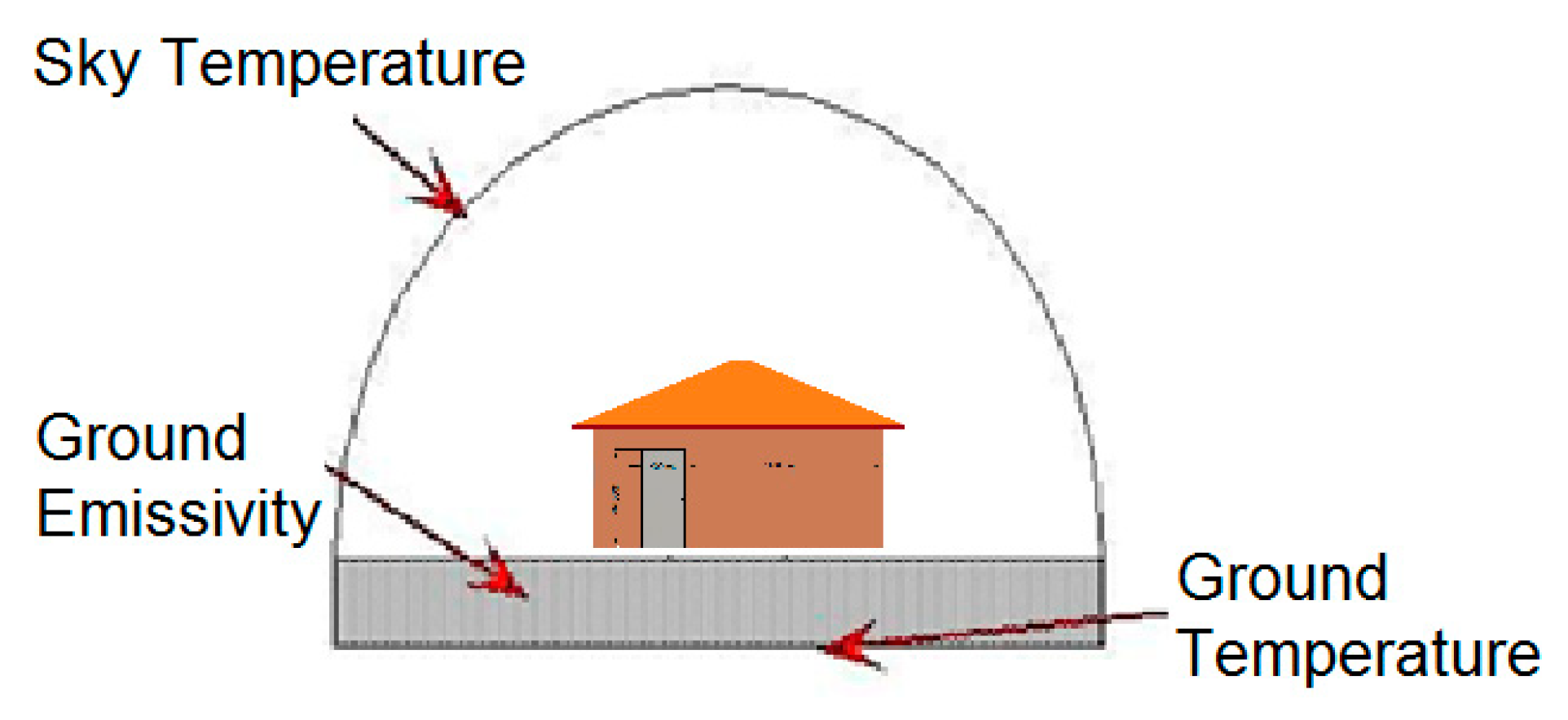
For the effective simulation of the effects of reflected and emitted radiated thermal exchange between the structure and its environment utilising CFD analysis, the height of the developed module was extended 10 times by cube environments and the module and the ground were completely enclosed, as illustrated in Figure 6 [27].

The geometrical characteristics of each module and material properties were modeled using the CFD environment. A large external environment of a 100 m × 100 m × 100 m external volume in the shape of a sphere to surround the building was constructed in CFD. Then the material properties for each module were assigned with the same thermal properties as the real modules. An automatic mesh was generated for analysis of the modules using an automatic topological examination for entire geometry to find the distribution of nodes and the mesh size. In this analysis, 264,534 nodes and k-epsilon turbulence modeling were used. Finally, a grid independence test was conducted to ensure the CFD simulation accuracy. The temperature and emissivity boundary for both the sky and ground were specified, as illustrated in Figure 6 [27].

The sky radiation temperature was applied to the dome’s outside surface. This temperature is generally within a limited range, approximately between 0 and 30 °C, which does not refer to the air temperature. At night-time, the sky temperature decreases to around 0 °C on nights with extreme cloudiness in warm environments, whereas on cloudless nights in cold environments, the sky temperature can even be reduced to −15 °C [27].

2.4. Calculating Sky Temperature Numerically

Sky temperatures were needed for buildings simulation programs such as Autodesk CFD and EnergyPlus. To calculate sky temperature the horizontal infrared radiation intensity (Horizontal_IR) in Wh/m² is needed and can be calculated [29,30] as following:

Horizontal_IR = ε σ T⁴

(1)

where;

Horizontal_IR = horizontal infrared radiation intensity (W/m²)

σ = Stefan–Boltzmann constant = 5.6697 × 10⁻⁸ (W/m²·K⁴)

T = dry bulb temperature (K)

ε = sky emissivity (0 < ε < 1) is given by

$${\mathrm{SKY}}_{\mathrm{emissivity}}=\left(0.787+0.767 \times \ln \left(\frac{{\mathrm{Temperature}}_{\mathrm{dewpoint} }}{273}\right)\right)+0.0224\mathrm{N}-0.0035{\mathrm{N}}^2+0.00028{\mathrm{N}}^3$$

(2)

where;

Temperature dewpoint = dewpoint temperature (K)

N = opaque sky cover (tenths), where sky cover: the expected amount of opaque clouds covering the sky valid for the indicated hour where N equals 0 for clear sky and 10 for overcast sky.

The default calculation for sky temperature can be calculated from the horizontal infrared radiation intensity as follows [31,32]:

Sky Temperature = (Horizontal_IR/σ) × 0.25 − Temperature(Kelvin)

(3)

where:

Sky Temperature = sky radiative temperature (°C).

Horizontal IR = horizontal infrared radiation intensity (Wh/m²).

Temperature (kelvin) = Temperature conversion from kelvin to celsius (273).

Calculating sky temperature numerically for each month to compare it with CFD results. Daily sky temperature changes is minimum which can be presented in monthly bases, the calculation for August will be presented in detail here; clear sky (N = 0.5), temperature dry bulb = 10 °C, temperature dewpoint = 4 °C.

Now the sky temperature can be calculated.

Temperature dry bulb = 273 + 10 = 283 K

Temperature dew point = 273 + 5 = 278 K:

Sky emissivity = 0.8

Horizontal IR = 0.8 × 5.669710-8 × (2834) = 291 W/m²

Sky Temperature = (Horizontal_IR/σ) × 0.25 − 273 = 267.7 − 273 = −5.3 °C (for August winter).

The lack of specific sky temperature equations for all areas of the world leads to the impossibility in determining the best existing formula but the comparison among the models can be useful to address the choice of users in building energy simulations and engineering applications. It was found that heating and cooling annual energy demands can be affected by significant percentage differences, ranging from −10% to +19% for tropical climatic conditions, from −10% to +13% for dry climatic conditions, from −19% to +28% for mild temperate climatic conditions and, finally, from −43% to +83% for snowy conditions [16].

3. Results and Discussion

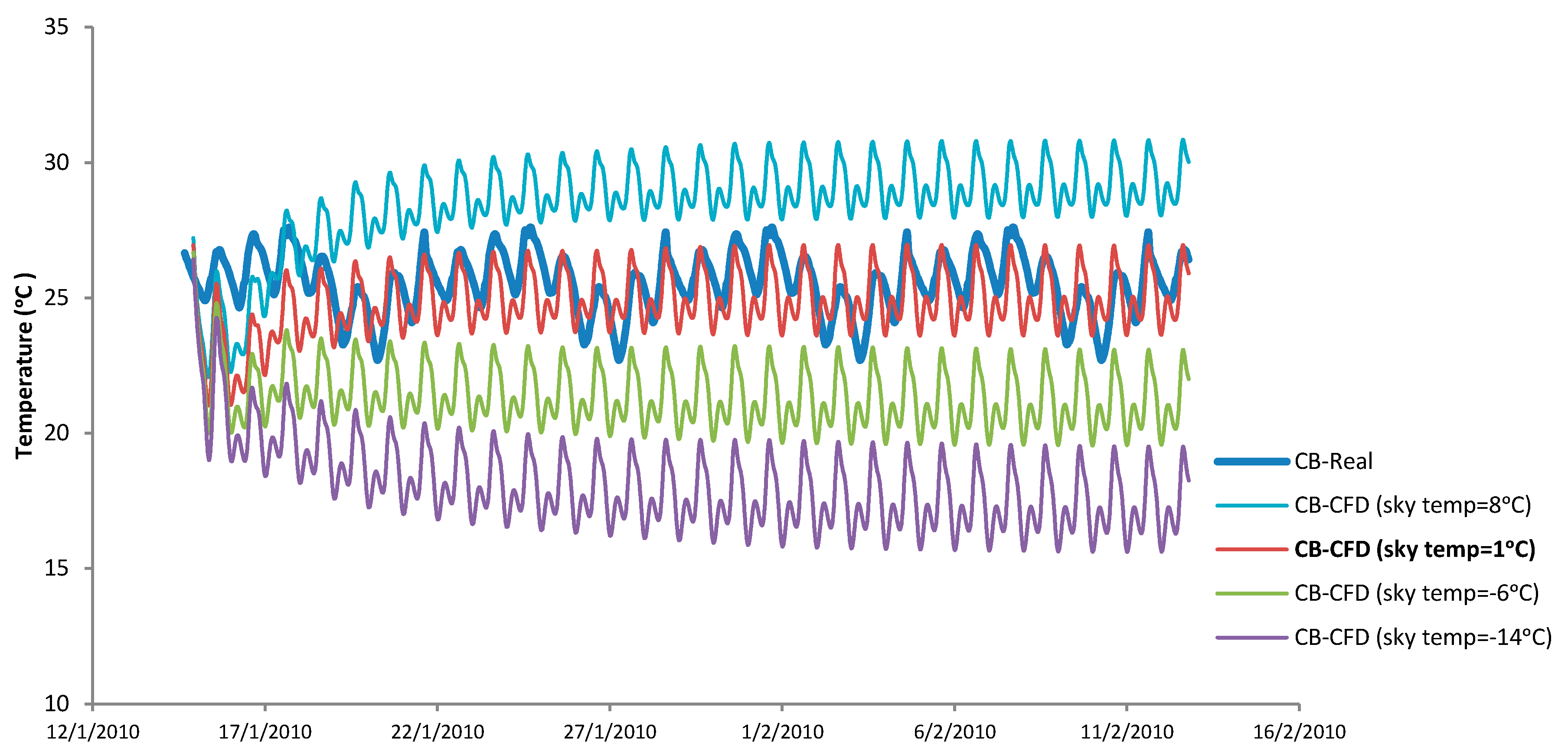
Real data obtained from real size house modules were used to find the effect of different sky temperatures on the building internal air temperature using CFD simulation. For example the cavity brick module (CB) were analysed for one month in summer (14 January 2010 to 13 February 2010) using 8 °C, 1 °C, −6 °C and −14 °C sky temperatures as shown in Figure 7.

This simulation indicates that higher sky temperature will result in higher internal air temperature where each 2 °C increases in the sky temperature will increase the average internal air temperature by almost 1 °C and decreases the sky temperature by 2 °C will decrease the average internal air temperature by 1 °C.

The sky temperature of 8ºC increases the internal air temperature of the building but the sky temperature of −6 °C and −14 °C decreases the internal air temperature as shown in Figure 7. Therefore, the closest simulated results to the real data occurred for the sky temperature of 1 °C.

The temperature inside the building increases or decreases in faster rate for the first week before it is stabilized, so the trend in the first week is representative while the effect of the sky temperature is considered.

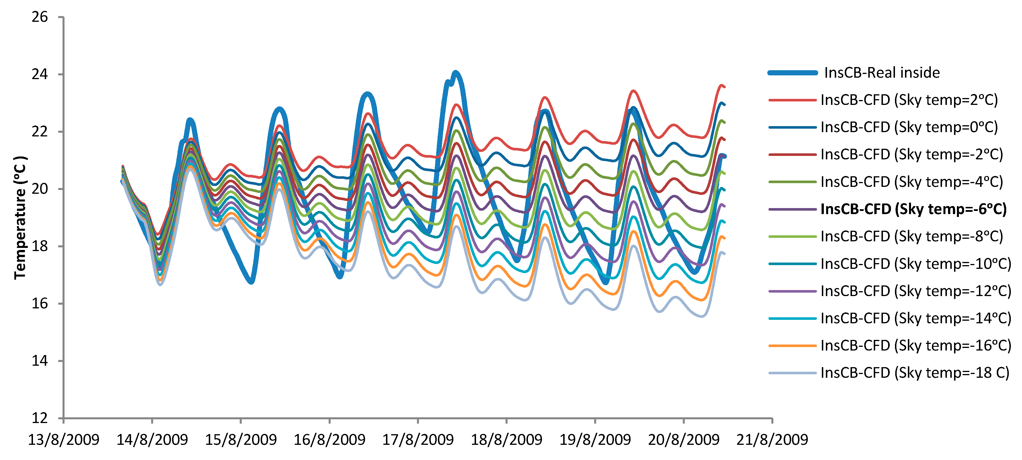
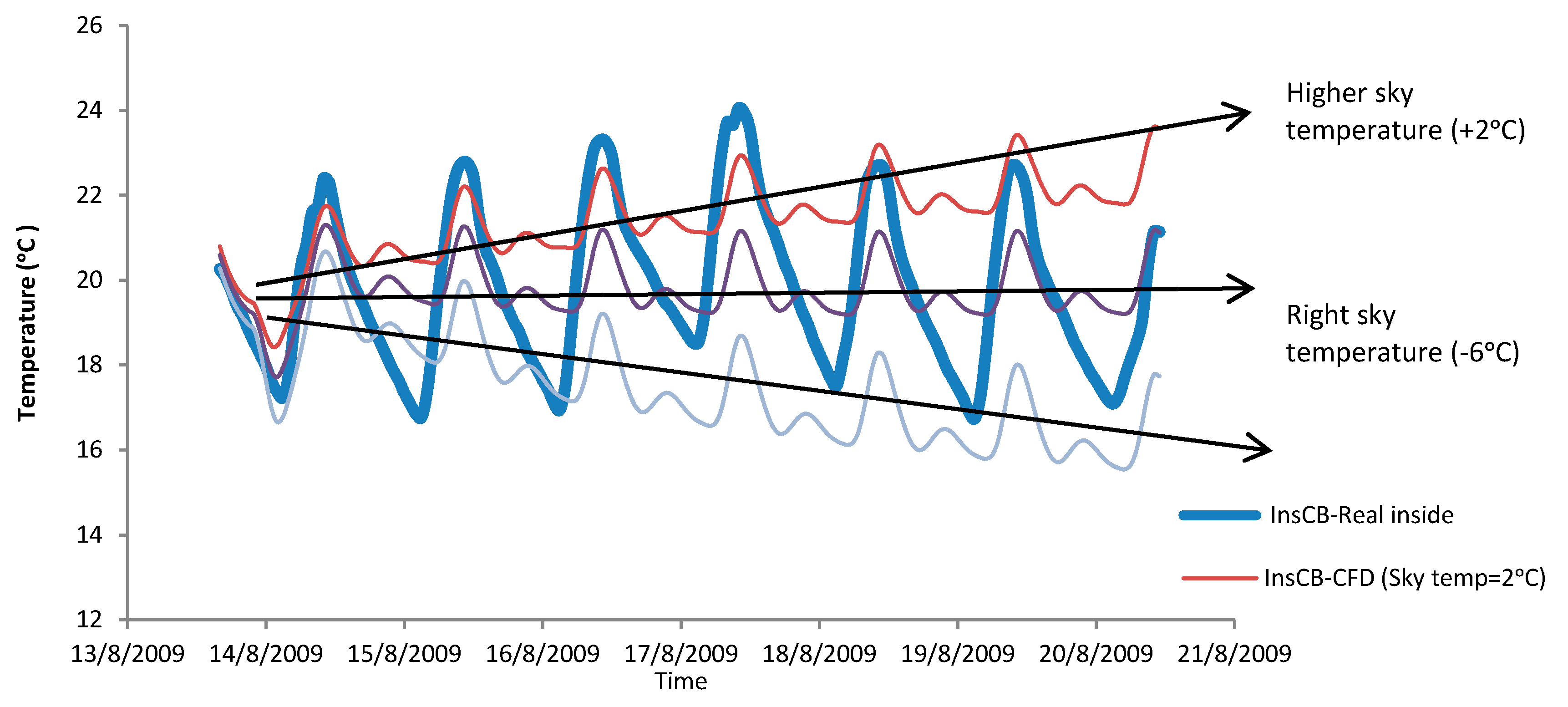
A one-week period was used here to determine the building internal air temperature for various sky temperatures. This is shown in Figure 8 for the InsCB module as an example.

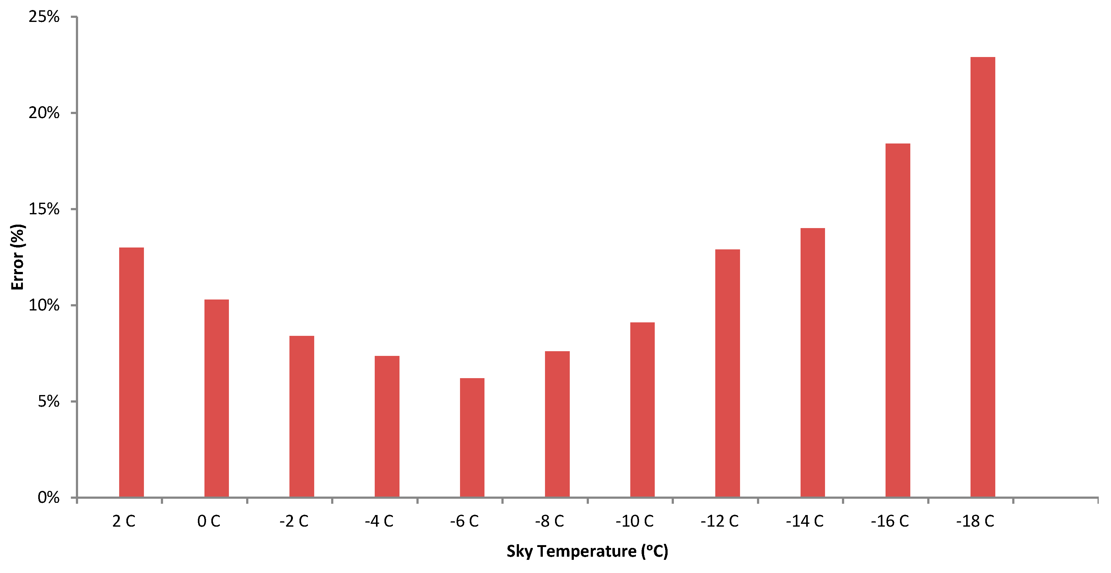
The sky temperatures of 2 °C, 0 °C, −2 °C and −4 °C, (which is higher by 8, 6, 4 and 2 °C accordingly than the accurate sky temperature of −6 °C) increased the internal air temperature of the module for August 2009 (see Figure 9). However, the sky temperature of −8 °C, −10 °C, −12 °C, −14 °C, −16 °C and −18 °C (lower by −2, −4, −6, −8, −10 and −12 °C accordingly than exact sky temperature of −6 °C) decreased the internal air temperature of the module as is shown in Figure 10. The average errors of the internal air temperature for various sky temperatures for the InsCB module is shown in Figure 9; the smallest error of 6.2% occurred for the sky temperature of −6 °C (accurate sky temperature) with similar trend as the observed internal air temperature for the module.

The most accurate (exact) sky temperature for August, calculated manually was −5.3 °C and −6 °C when simulated by CFD (i.e., the trend of the simulation line up with observed internal air temperature). The sky temperature higher or lower than 6 °C will increase/decrease module internal air temperature as shown in Figure 10.

The smallest error of 6.2% occurred when the sky temperature used in the CFD simulation was close to the manually calculated sky temperature of −5.3 °C. However the sky temperature of +2 °C and −18 °C increased the error between observed and CFD internal air temperature to 13% and 22.9% respectively.

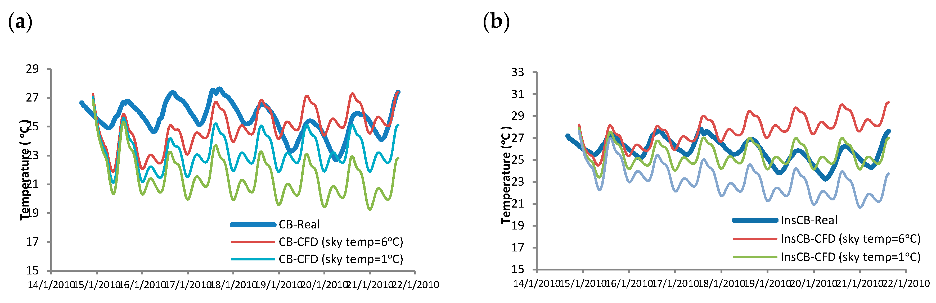
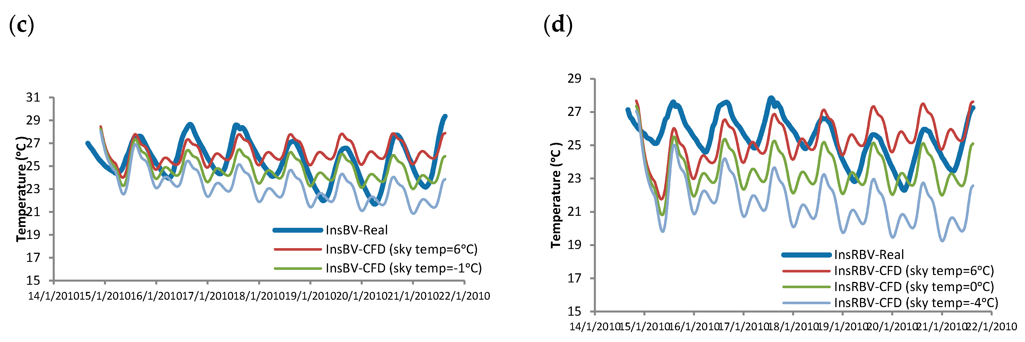
It should be noted that the sky temperature was supposed to be similar for all modules and this hypothesis was analysed for one summer week in January 2010 and presented in Figure 11. The most accurate sky temperature fell within 1 °C, 1 °C, −1 °C and 0 °C for the CB, InsCB, InsBV and InsRBV, respectively. The difference between the highest and the lowest sky temperature is less than 2 °C between the modules.

The magnitude of the error between the CFD results and the real data largely depends on the accuracy of the sky temperature and how close it is in value to the accurate sky temperature where 5 degrees difference with the right sky temperature will result in almost double the error over one month (for 5 °C higher result in 10.2%, 10.4%, 9.4%, 9.3% error and for 5ºC lower result in 13.3%, 15.1%, 14.7%, 13.9% error for the CB, InsCB, InsBV and InsRBV, respectively).

Note: three sky temperature values were only presented in Figure 11 (i.e., high sky temperature of 6 °C, right sky temperate with least error compared to the real data and low sky temperature of −4 °C).

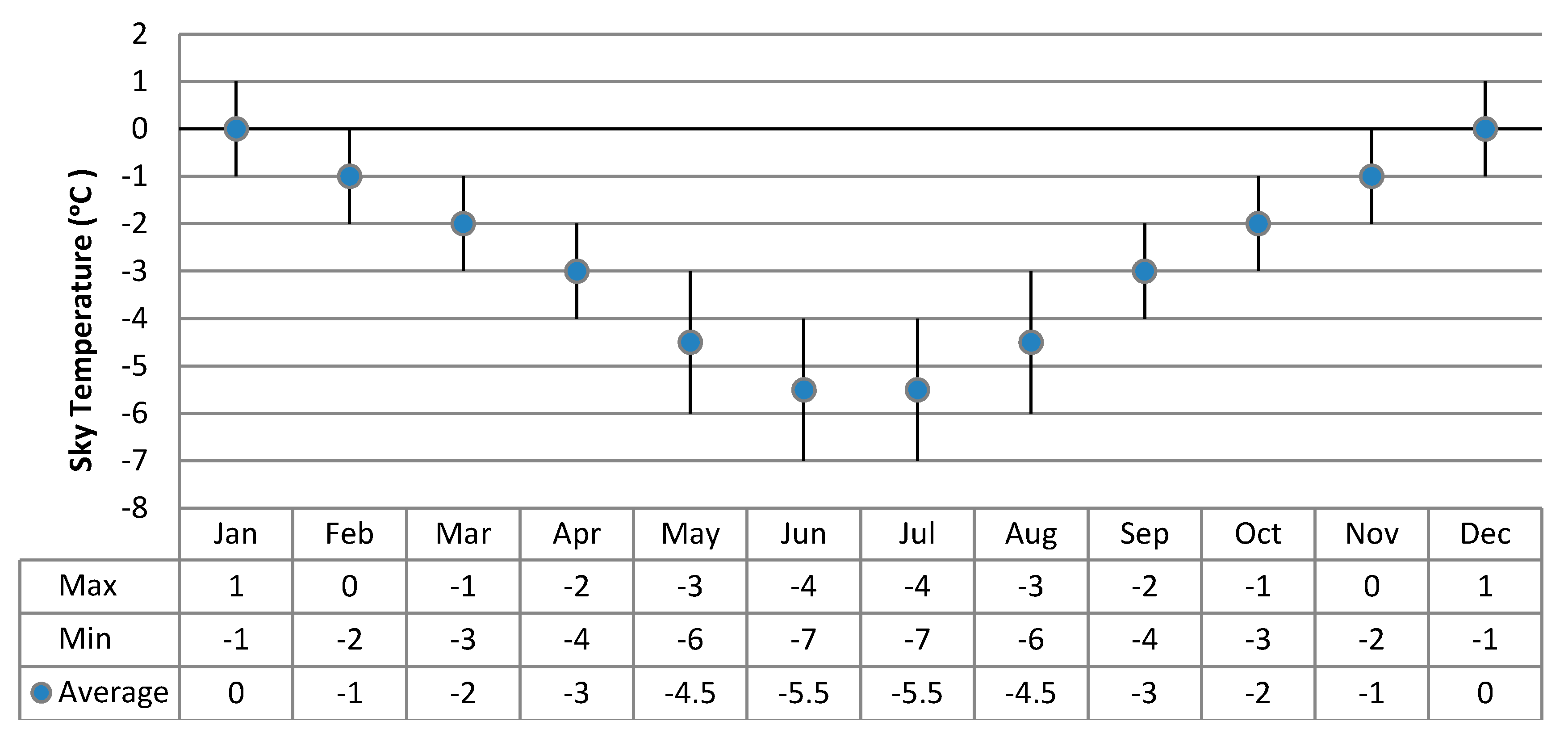
The monthly sky temperature varies throughout the year from 1 °C in January to −7 °C in July and the difference for each month between the modules varies from 2 °C to 3 °C as shown in Figure 12.

The monthly sky temperature was determined in two methods; i.e., numerically and using CFD simulation for each module where the average simulated sky temperatures are close to the calculated sky temperatures (see

Table 1. Errors between CFD simulations and real data using different sky temperatures.

	CB	InsCB	InsBV	InsRBV
Higher sky temperature by +10 °C	16.5%	17.5%	17.1%	16.8%
Higher sky temperature by +5 °C	10.2%	10.4%	9.4%	9.3%
Higher sky temperature by +2 °C	7.2%	7.4%	6.9%	6.8%
Exact sky temperature	6.5%	7.1%	6.2%	6.4%
Lower sky temperature by −2 °C	8.3%	9.1%	8.7%	8.9%
Lower sky temperature by −5 °C	13.3%	15.1%	14.7%	13.9%
Lower sky temperature by −10 °C	19.3%	22.6%	21.9%	19.1%

) with a maximum difference of 1.1 °C. The average monthly sky temperatures for the temperate climate in Newcastle, Australia, for all the modules are presented in

Table 2. Difference in the sky temperatures between CFD analysis and calculated values.

Month	CFD Average (°C)	Calculated (°C)	Difference (°C)
January	0	0.6	0.6
February	−1	−1.1	0.1
March	−2	−2.3	0.3
April	−3	−3.7	0.7
May	−4.5	−5.3	0.8
June	−5.5	−6.6	1.1
July	−5.5	−6.6	1.1
August	−4.5	−5.3	0.8
September	−3	−3.7	0.7
October	−2	−2.3	0.3
November	−1	−1.1	0.1
December	0	0.6	0.6

.

Table 2 shows the error between CFD results and real data (for 12 months’ simulation) using sky temperatures higher and lower by 2 °C, 5 °C and 10 °C. Using the right sky temperature value for each module CB, InsCB, InsBV and InsRBV will result in 6.5%, 7.1%, 6.2% and 6.4% error, correspondingly, compared with the real data. These errors mainly refer to the simulation error.

Using higher sky temperatures by +10 °C will significantly increase the error to 16.5%, 17.5%, 17.1% and 16.8% and lower sky temperature by +10 °C will also increase the error to 19.3%, 22.6%, 21.9% and 19.1% for CB, InsCB, InsBV and InsRBV modules, respectively.

Using the right sky temperature will minimize the differences between simulated results and the real data. For example using the right sky temperature for February (1 °C, 1 °C, −2 °C and 0 °C for the CB, InsCB, InsBV and InsRBV modules, respectively) will result in 5.4%, 6.1%, 5.9% and 6.1% error, correspondingly, compared with the real data. These errors mainly refer to the simulation error. On the other hand, using other sky temperature values will significantly increase the error.

4. Conclusions

An accurate sky temperature used in CFD simulations or another buildings energy assessment program (e.g., EnergyPlus) is necessary to reflect the real performance of the buildings. Otherwise, this may lead to incorrect assessment of the existing or new buildings’ thermal performance, operating energy, and GHG emission over the entire life-span.

In this paper, the effect of the different sky temperatures on buildings was compared between the real data for four real-sized test buildings and the CFD simulation results. The monthly sky temperature was determined by two approaches; i.e., numerically and using CFD simulation with less than 1.1 °C difference. The sky temperature varies throughout the year but it was found that monthly sky temperature provides a reasonable degree of accuracy for building thermal simulation. It seems to be unnecessary to input a weekly or even daily sky temperature which would require 52,365 separate calculations.

It was found that inaccurate sky temperature (10 °C higher or lower than the exact sky temperature) will lead to an average error of more than 20% (3 times more compared with the accurate value for the sky temperature) of internal air temperature for a building. However, the error decreases to about 6% (mainly due to simulations errors) when the exact temperature is applied.