1. Introduction
Peripheral nerves are crucial to connect sensory and motor organs to the central nervous system [
1,
2]. Motor nerves carry information towards organs, muscles, or other peripheral effectors, and also, sensory nerves link sensory receptors to the brain [
3]. These complex structures are hierarchically organized: internal axons, together with Schwann cells, are protected by a loose connective tissue (i.e., the endoneurium), which was found to be mainly composed by I and II type collagen, macrophages, and mast cells and filled by endoneurial fluid [
2,
4,
5]. Endoneurial components are, in turn, enveloped in fascicles by the epineurial sheet, which is formed by layers of perineural cells, I and II type collagen, together with elastic fibers [
2,
4,
5]. Finally, fascicles are grouped together by a further layer of connective tissue (i.e., the epineurium) mainly composed by I and III type collagen, elastic fibers, and mast and fat cells [
2]. Despite this richness of internal substructures, the main constitutive components of the connective tissues of nerves are elastin and collagen, which were found to be mainly axially oriented [
4].
In addition, peripheral nerves are physical objects, which obey physical laws [
6]. Indeed, they react to external mechanical stimuli trough a specific mechanical response, increasing their stiffness to keep axons’ integrity and to preserve endoneurial structures from longitudinal overstretch [
7]. The knowledge and the prediction of this kind of response are important in medicine [
8,
9] and physical therapy [
2,
10,
11], while they are strategic in modern and high-tech bioengineering fields, as in neural interfaces design [
12,
13,
14].
Although the anatomic path of nerves involves branching points, their mechanical response to longitudinal stretch was closely related to the response of the rectilinear nerve trunks [
7]. As a consequence, and for the sake of simplicity, different kinds of models were implemented to predict the rectilinear nerve trunk response to external stimuli. Indeed, from one side, peripheral nerves were modeled as isotropic materials, providing a deterministic elastic [
15,
16] or hyperelastic response [
17,
18,
19,
20,
21]. From the other side, a stochastic iterative fibril-scale mechanical model was implemented to reproduce the straightening of wavy fibrils and to account for the effects of interfibrillar crosslinks on the overall properties of the tissue [
22,
23]. Furthermore, recent studies aimed at investigating the relationship between macroscopic tensile loading of nerves and micro-scale deformations [
24].
Nevertheless, a deterministic and explicit continuum model to explore the influence of the ground matrix and collagen fibrils on the nerve stiffening is apparently not available in literature. As a consequence, in this work, such a theoretical framework is provided to quantify the action of both the ground matrix and collagen fibrils on the nerve stiffening.
In particular, the text is organized as follows: First, a closed-form strain energy function (SEF) is proposed to account for the actions of the matrix and fibrils. Then, the change of the shape of the stress/stretch curve is studied for variations of relevant numerical parameters, while a further sensitivity study is performed. Finally, the proposed framework is used to investigate the stiffening phenomenon in different nerve specimens coming from different animal models [
19,
25].
2. Methods
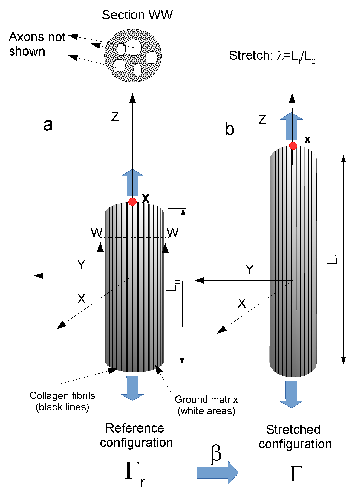
The peripheral nerve was modeled as a three-dimensional continuum body (elliptic cylinder), which was deformed into a final configuration
starting from a reference configuration
. The position of each point of this solid was identified through the vectors
and
, respectively related to the reference and the deformed configuration. As shown in
Figure 1 below.
The deformation of the body was described through a time-dependent map
, where
is an invertible and regular function. Unlike previous models [
17,
18,
19,
20,
21,
22,
23], a unit vector field
was used to explicitly account for the presence of the collagen fibrils in the reference configuration
[
26,
27]. For the sake of simplicity, the collagen fibrils were modeled as axially oriented with no dispersion [
4].
The response of the nerve was described through a strain energy function
(per unit of volume), which was affected by the initial fibrils’ direction, as well as by the strain measure. Therefore, the mean Cauchy stress tensor within the nerve is written as:
where
is the deformation gradient,
, and
is the right Cauchy–Green strain tensor.
In particular, an invariant-based form of this energy is used:
where,
,
,
,
,
. The Cauchy stress tensor is, then, better specified as:
where
is the left Cauchy-Green tensor,
,
,
. As in previous literature [
7,
19,
20,
21], the nerve was considered incompressible (i.e., the nerve volume remained the same, when the specimen underwent deformation), then
, and the pressure contribution within the Cauchy stress tensor was made explicit. Thus, the stress is written as:
where
p is the hydrostatic pressure, while
is the unit tensor. The physical behavior of the nerve was assumed to result from the contribution of the main structural components of its connective tissue, that is the elastin matrix and the collagen fibers. Therefore, to account for both their action, the strain energy function is written as:
where
is the energetic term due to the ground elastin matrix, while
is the energetic term describing the collagen fibrils.
As a consequence,
, since
is independent of
and
, and the Cauchy stress tensor is further simplified as:
More specifically, the energetic contribution of the matrix is written as [
28]:
where
. In contrast, the energetic contribution of the collagen fibrils is derived from:
where
and
. In addition,
are numerical parameters, while
, and (
) is a real function, a continuum with its n-th order derivatives. Here, for the sake of simplicity,
[
29,
30], and
.
Since the nerve was axially stretched, its lateral surface was stress-free, and
. Therefore, the contributions of the axial Cauchy stress due to the matrix and to the fibrils are written as
and
, respectively. However, in the following, these contributions will be simply written as
and
, dropping the
index related to the direction of stretch (
z axis). Similarly, in the following, the longitudinal stretch is
, where
is the initial length of the specimen, while
is the final length of the nerve after the axial stretching. Recalling this notation, the axial stress due to the action of the matrix is:
while the axial stress due to the fibrils’ action is:
where
and
. Similarly, their rates of change with stretch are:
while their second derivatives with respect to
are:
where
. As a consequence, the total amount of stress within the nerve, together with its derivatives, are written as:
Furthermore, the partial amount of nerve stiffening due to each component (matrix and fibrils), as well as the total amount of nerve stiffening were measured through the extrinsic curvature of each stress/stretch curve. In particular, the dimensionless extrinsic curvature due to the matrix-derived stress/stretch curve, accounting for the stiffening due to the ground matrix action, is written as:
where:
In contrast, the extrinsic curvature of the fibril-derived stress/stretch curve was studied through two different formulas. The first one is written as:
where:
and accounts for the nerve stiffening due to the collagen fibrils’ action, while the second one is written as:
where:
and measures the amount of the nerve stiffening due to the collagen action with reference to the stiffening due to the matrix action. In addition, the total dimensionless stress in the nerve is written as:
while the total dimensionless curvature of the stress/stretch curve, accounting for the coupled action of matrix and fibrils, is defined as:
Once having defined the previous theoretical framework, the range of variation of Equations (
9) and (
10) was explored by changing their main numerical parameters (i.e.,
) through the auxiliary set
, to test their suitability for reproducing the classic evolution of the stress/stretch curve [
2,
7]. Moreover, to assess their quantitative dependence on the numerical parameters, a sensitivity study was performed through the index [
31,
32]:
where
q is the studied quantity,
is the output value of
q derived from the variation of the chosen parameter
, while
is the reference value, when all the parameters are set to 1. The further the resulting value of Equation (
26) was far from zero, the more the effects of the studied parameter affected the quantity
q.
Finally, theoretical predictions were compared to experimental data collected from five consecutive extensions of a porcine peroneal nerve [
19] and for one extension of a canine left vagus nerve [
25]. More specifically, Equation (
15) was used to reproduce the experiments, while numerical parameters were optimized through a non-linear procedure (quasi-Newton algorithm, Scilab; Scilab Enterprises S.A.S 2015), allowing the
statistic to be maximized and residual plots minimized for each extension. Once having obtained the relevant parameters (
) for the real experiments, Equations (
18)–(
25) were used to explore the action of the ground matrix and the collagen fibrils on the stiffening of the nerve during axial stretch.
3. Results
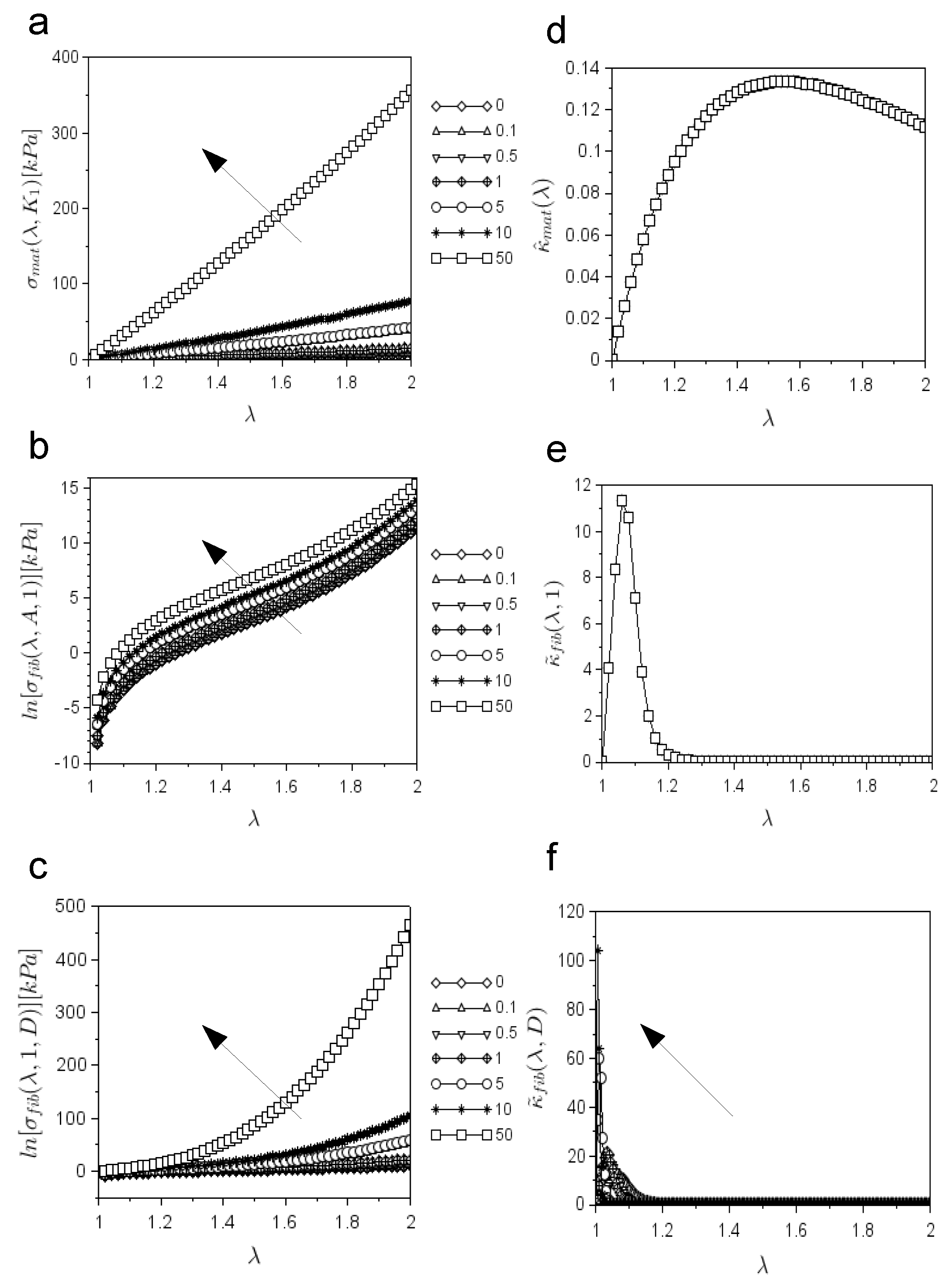
To explore whether, as a matter of principle, the previous framework was able to reproduce the classic evolution of the nerve stiffening phenomenon, the range of variation of the main theoretical curves was studied. First, the range of variability of Equation (
9), accounting for the stress due to the matrix contribution (
Figure 2a), was investigated for increasing values of
. In particular, the values of
were computed for
. For a small stretch (i.e.,
), Equation (
9) reduced to
, so the initial slope of the curve was
.
Then, Equation (
10), accounting for the stress derived from the collagen fibrils’ contribution, was investigated for
and
,
. Larger values of
A resulted in larger values of
(as shown in logarithmic scale in
Figure 2b), while for
, its slope was
. The contribution of fibrils was also investigated for
and for different values of
,
, through the evolution of the natural logarithm of
(
Figure 2c). More specifically, the larger the value of
D was, the more the value of fibril stress increased, while for
, its slope was
.
In addition, Equation (
18), accounting for the stiffening due to the matrix action
, monotonically increased for
, while after a maximum
, it monotonically decreased for
(
Figure 2d). For
, its slope was
.
Similarly, Equation (
22), accounting for the stiffening due to the action of fibrils, for
(i.e.,
), had a fixed bell-like shape (
Figure 2e), with a maximum
. Its full width at half maximum was FWHM
, while for
, its slope was
. On the contrary, the same Equation (
22) for different values of
,
(i.e.,
), had a variable bell-like shape (
Figure 2f). The larger the value of
D was, the more the value of the peak increased, while the more the value of the FWHM
decreased. In other words, for
,
, while FWHM
. However, these curves had the following characteristic:
,
. Furthermore, for
, its slope quadratically increased with D, since it was
.
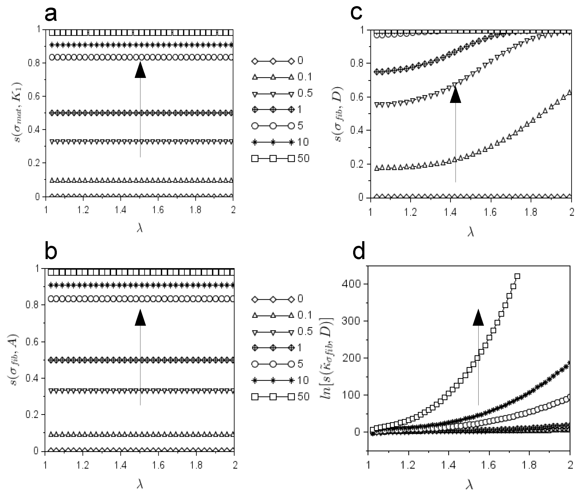
To better quantify the influence of each parameter, a sensitivity study was also performed on each contribution. More specifically, the sensitivity of
with respect to changes in
was tested in
Figure 3a. Since it was found that
, the larger the value of
(
) was, the more the value of its value converged towards one.
Again, the effects of the changes in
A or
D were investigated on the stress functions due to the collagen fibrils. In this case as well, it was found that
, (
Figure 3b), for different values of
,
. Thus, the larger the value of
A was, the more the value of
converged towards one. Similarly, the evolution of
is shown in
Figure 3c for different values of
,
. The larger the value of
D was, the quicker the value of
converged towards one. On the contrary, the larger the value of
D was, the quicker the function
diverged, as shown in
Figure 3d.
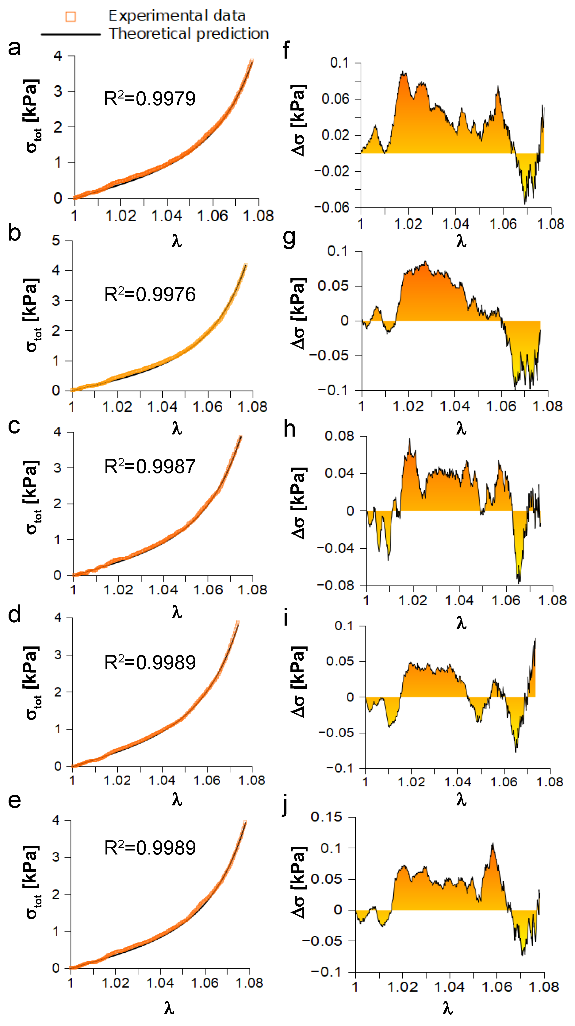
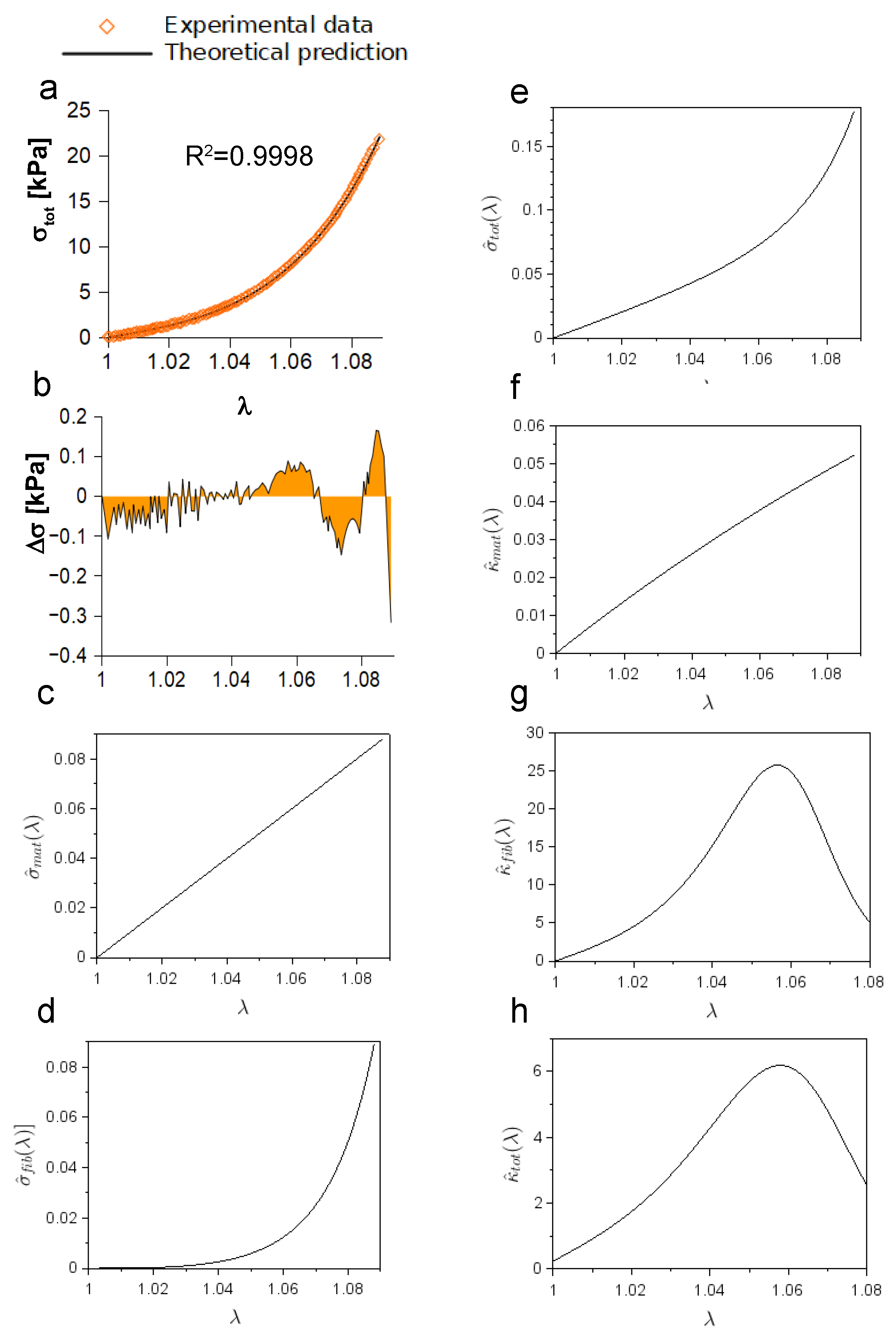
Once having tested the suitability of the provided framework, Equation (
15) was used to study the experimental response of a porcine peroneal nerve (five consecutive elongations up to
) [
19]. Stress data are reported as a function of stretch (
Figure 4) and quantitatively compared to theoretical predictions through the
statistic and the computation of residuals (
). This comparison resulted in
for the first elongation (
Figure 4a),
for the second one (
Figure 4b),
(
Figure 4c–e). Similarly, residuals ranged between
kPa and
kPa for the first elongation (
Figure 4f), while they ranged between
kPa and
kPa for the second one (
Figure 4g). Moreover, residuals spanned from
kPa to
kPa (
Figure 4h), from
kPa to
kPa (
Figure 4i), and from
kPa to
kPa (
Figure 4j), for the third, fourth, and fifth elongation, respectively. Finally, relevant quantities (mean ± standard deviation) in Equation (
15) were quantified and resulted in
kPa,
kPa, and
.
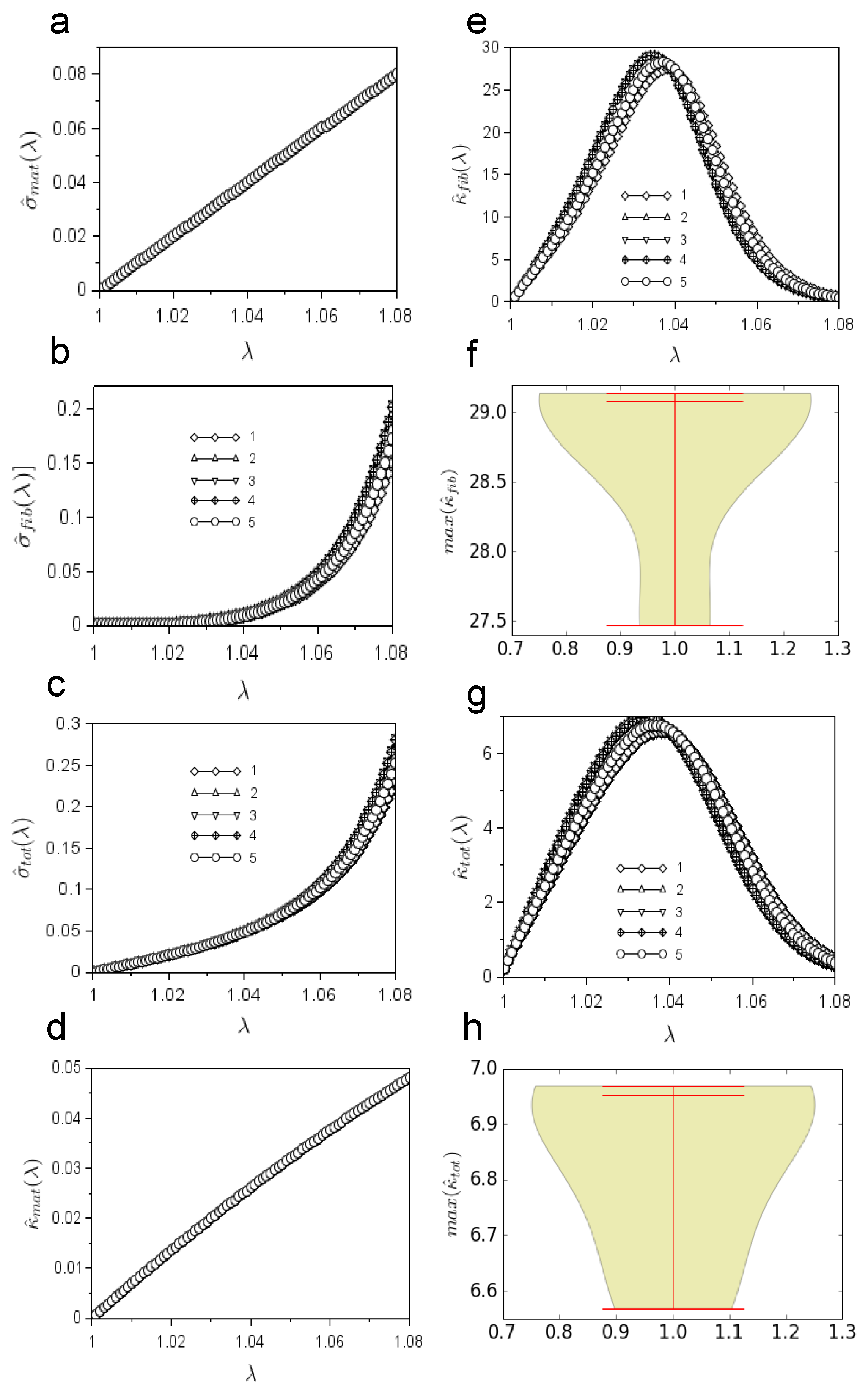
Moreover, the dimensionless stress and curvature were investigated. In particular, the dimensionless stress due to the matrix contribution (
) monotonically increased from zero (
) to
(
,
Figure 5a). The slope of
was (mean ± standard deviation)
for
, while it was zero by definition at
(
Figure 5b). Similarly, the slope (mean ± standard deviation) of the total dimensionless stress
was
, at
, while, by definition, the slope was one at
(
Figure 5c). The dimensionless curvature
monotonically increased from zero (
) up to
(
) with a slope of about
(
Figure 5d). On the contrary, the dimensionless curvature due to the fibrils’ action
had a bell-like shape (
Figure 5e). In particular, this curve reached its maximum value (mean± standard deviation)
at
. The median, maximum, and minimum values of
were, respectively
, as shown in
Figure 5f, together with the shape of their distribution. Finally,
is studied in
Figure 5g. In this case as well, the curve had a bell-like shape and reached the maximum value of
at
. The median, maximum, and minimum values of
were respectively
, as shown in
Figure 5h, together with their distribution shape.
The proposed framework was also used to explore experimental data derived from the axial stretching of a canine left vagus nerve [
25]. In this case, Equation (
15) with
kPa,
kPa,
, was able to closely reproduce the experiments (
,
Figure 6a), while residuals (
) spanned from
to
(
Figure 6b). The dimensionless stress due to the action of the matrix linearly increased from zero (
) to
(
), and the slope of this curve was
for
, as shown in
Figure 6c. On the contrary, the dimensionless stress due to fibrils increased in a non-linear way from zero to
, and the slope of this curve increased from zero (
) to
(
) (
Figure 6d). Similarly, the total dimensionless stress increased in a non-linear way from zero to
, and its slope spanned from
(
) to
(
), as shown in
Figure 6e. Furthermore, the dimensionless curvature
monotonically increased from zero (
) up to
(
) (
Figure 6f), while the dimensionless curvature due to the fibrils’ action
had a bell-like shape (
Figure 6g). In this case, the maximum value of the curve was
, which was reached at
. Finally,
was studied. This curve had a bell-like shape, and the maximum value was
at
, as shown in
Figure 6h.
4. Discussion
To tackle nerve neuropathies deriving from different kinds of pathologies (i.e., diabetes, scleroderma) [
33], dietary deficiency, or exposure to ionizing radiation (e.g., neuromalacia) [
34], an explicit understanding of the main features of the peripheral nerve response to stretch is needed. In particular, a computationally light and physically-based theoretical approach, linking in a deterministic and explicit way the main physical constituents of the connective tissue to the macroscopic response of the peripheral nervous tissue, could be strategic to make quantitative and reliable predictions.
Since peripheral nerves are anatomically complex (i.e., they have branching points), but their overall response is closely related to the response of their main rectilinear tract (which is the main structural segment), in this work, they were modeled as continuum rectilinear transverse isotropic bodies. Indeed, although peripheral nerves are hierarchically organized, ultrastructural studies revealed that the main constituents of the connective tissue are a ground matrix of elastin and a longitudinally-oriented fibrous network of collagen [
4]. As a consequence, the strain energy function, ruling the nerve behavior, was dominated by
and
, that is by the energetic contributions of the matrix and fibrils, respectively.
In particular, the energetic contribution of the elastic ground matrix was modeled through a first order Yeoh-like strain energy function [
28], while the energetic contribution of the collagen fiber network was modeled through Equation (
10), where, for the sake of simplicity, the function
was a convex energy function, traditionally used to model the behavior of soft tissues [
29,
30]. The superimposition of these energetic contributions was able to closely reproduce the experimental evolution of the mean Cauchy stress.
First, to qualitatively test the suitability of the provided approach, changes in numerical parameters were investigated with respect to their effectiveness in reshaping both the and curves. In particular, with reference to , the more increased, the steeper the stress curve was, due to the action of the ground matrix. Similarly, the steepness of increased in a linear way by increasing the A value, since it resulted in a proportional magnification of the curve. On the contrary, D affected in a highly non-linear way.
In the same way, the dimensionless extrinsic curvature
showed that the contribution of the ground matrix to the nerve stiffening was limited with stretch, while
heavily affected the stiffening process. As a consequence, three parameters were enough to provide a variety of shapes, allowing experimental trends to be correctly reproduced by theoretical predictions, while in the literature, more parameters were needed to account for the collagen action through an iterative and probabilistic approach [
22,
23].
In addition, the sensitivity of and and towards changes in numerical parameters was explored. In particular, the sensitivity of the matrix stress function to the variation of and the sensitivity of the fiber stress function to the variation of the A parameter (with respect to the unit values of the other constants) converged towards zero for increasing values of and A. On the contrary, the sensitivity of the fibril stress function ( to the variation of the D parameter quickly reached the steady value of one. The higher the value of D was, the faster the steady state was reached. As a consequence, the parameter D affected more extensively than the parameter A. In contrast, A affected exactly as affected . The sensitivity of to variations of the parameter D resulted in a highly non-linear and diverging line. The more the value of D increased, the more the line diverged. In other words, the value of D heavily affected the curvature of the stress due to the collagen action.
The parameter
was, then, physically related to the apparent stiffness of the nerve for small strain (in this case, the Young modulus was
), while the parameter
A controlled the linear part of stress increment due to the collagen action. Furthermore, the parameter
D affected the curve steepness and controlled both the delay (with respect to the reference configuration) and the velocity of the nerve stiffening process. Therefore, it was shown, as a matter of principle, that the proposed deterministic and explicit framework, exploiting closed-form equations with three main parameters, was able to reproduce the classic nerve stiffening behavior [
2,
7].
As a consequence, first, this framework was used to explore the stiffening behavior of real specimens. Indeed, with reference to the porcine peroneal nerve, theoretical predictions were able to closely reproduce the experiments (), while residual plots were analyzed to avoid numerical bias (e.g., over-fitting) keeping the value of the statistic artificially high. All residuals (), between theoretical predictions and experimental values, were within kPa; that is, the error was about in the worst case, confirming that experiments were reproduced with confidence. To further explore the response of the porcine nerve, dimensionless stress and curvature were used, since the dimensionless stress was able to quantify the evolution of stress with respect to the stiffness of nerve for small strain, while the dimensionless curvature was used to measure the nerve stiffening, since it mapped where and how much the dimensionless stress evolved non-linearly because of the action of collagen fibrils.
More specifically, the slope of
at
was on average 14 times greater than the slope at the reference configuration (i.e., at
), while the slope of
was practically constant. In addition,
was small with respect to
(i.e.,
). These results not only suggested that the stiffening process was dominated by the action of the collagen fibrils, confirming previous literature [
2,
7,
24], but also provided a quantification of the amount of the stiffening phenomenon (i.e., through the change of the slope by 14 times), as well as a quantification of how much the fibrils’ action was able to overcome the contribution of the ground matrix (i.e., about two orders of magnitude). On the contrary, the maximum dimensionless curvature of
was lower than the maximum curvature of
(i.e,
). This result suggested a possible lowering action of the ground matrix on the huge stiffening action of the collagen fibrils.
Furthermore, since the proposed framework was not intrinsically connected to any kind of animal or human model, it is, as a matter of principle, suitable to explore any kind of nerve. To show this, a different specimen, coming from a different animal model, was investigated. Indeed, with reference to a canine left vagus nerve, theoretical predictions were able to closely reproduce the experiments (), while all residuals were within kPa; that is, the error was less than . Furthermore, the slope of at was on average 12 times greater than the slope at the reference state (i.e., at ), while the slope of was practically constant. In addition, was small with respect to (i.e., ). Therefore, again, these results were able to quantify the stiffening phenomenon in a canine vagus nerve (change of the dimensionless total stress slope of about 12 times) and showed that the action of collagen fibrils dominated the nerve stiffening phenomenon (of about two order of magnitude). Moreover, since was lower than and there was , also in this case, a lowering action of the matrix with respect to the stiffening action of the collagen fibrils was suggested.
Curiously, for both specimens
, indicating the existence of common features between different species. More specifically, the analysis of dimensionless stress suggested that collagen fibrils were the main common structural features supporting the strain stiffening behavior. On the contrary, the analysis of the dimensionless curvature suggested a kind of common lowering action of the ground matrix on the huge stiffening due to the collagen fibrils’ action. In addition, although the model made abstraction of the real location of the collagen inside the nerve, it supported the hypothesis that the main structural contribution was performed by connective tissues in epineurium and perineural sheets [
7].
Finally, since the provided model was general, it was able to investigate the mechanical response of different nerves coming from different animal models (i.e., suine peroneal and canine vagus nerves). In both cases, the experimental evolution of stretch was closely reproduced (
) with small residuals. In other words, the provided framework was predictive, by definition, for the tested specimens, since
statistics were high and residuals small. However, it seems to be predictive also for human cadaveric specimens [
7] and for nerves coming from other animal species (i.e., rabbit [
35], lobster, aplysia, [
19,
36]), since the evolution of stress with stretch (or strain) is similar to the evolution of the studied specimens. In addition, the main theory was derived from biomechanical considerations; thus, the model seems to have also explanatory power with reference to a possible mechanism of action of elastin and collagen fibers.


